Article

Machine Learning-Based Flood Risk Assessment in Urban Watershed: Mapping Flood Susceptibility in Charlotte, North Carolina

1
School of Civil, Environmental, and Infrastructure Engineering, Southern Illinois University, 1230 Lincoln Drive, Carbondale, IL 62901-6603, USA
2
Department of Geomatics Engineering, School of Engineering, Kathmandu University, Dhulikhel 45210, Nepal
3
Department of Artificial Intelligence, Kathmandu University, Dhulikhel 45210, Nepal
*
Author to whom correspondence should be addressed.
Geographies 2025, 5(3), 43; https://doi.org/10.3390/geographies5030043
Submission received: 2 June 2025 / Revised: 8 August 2025 / Accepted: 11 August 2025 / Published: 18 August 2025

Abstract

Flood impacts are intensifying due to the increasing frequency and severity of factors such as severe weather events, climate change, and unplanned urbanization. This study focuses on Briar Creek in Charlotte, North Carolina, an area historically affected by flooding. Three machine learning algorithms —bagging (random forest), extreme gradient boosting (XGBoost), and logistic regression—were used to develop a flood susceptibility model that incorporates topographical, hydrological, and meteorological variables. Key predictors included slope, aspect, curvature, flow velocity, flow concentration, discharge, and 8 years of rainfall data. A flood inventory of 750 data points was compiled from historic flood records. The dataset was divided into training (70%) and testing (30%) subsets, and model performance was evaluated using accuracy metrics, confusion matrices, and classification reports. The results indicate that logistic regression outperformed both XGBoost and bagging in terms of predictive accuracy. According to the logistic regression model, the study area was classified into five flood risk zones: 5.55% as very high risk, 8.66% as high risk, 12.04% as moderate risk, 21.56% as low risk, and 52.20% as very low risk. The resulting flood susceptibility map constitutes a valuable tool for emergency preparedness and infrastructure planning in high-risk zones.

1. Introduction

Throughout the world, floods rank as the most destructive natural hazard, causing far-reaching economic costs, infrastructure destruction, and tragic loss of life [1,2]. The aggravating consequences of a changing climate have unmistakably heightened flood frequency and intensity, presenting significant challenges to communities worldwide [3]. Compounding these challenges are extreme weather patterns, sea-level rise, and urbanization, all of which drive greater vulnerability to floods [4]. Thus, developing accurate and dependable flood susceptibility models is no longer a choice but a necessity to mitigate possible losses effectively. The consequences of flooding extend far beyond the immediate physical destruction of vital infrastructure and the displacement of people; it also destabilizes local economies and causes long-term environmental deterioration, underscoring the imperative for proactive and innovative approaches to risk management [5].
Traditional flood susceptibility methods use static variables such as average rainfall, land use maps, and topography [6,7,8]. While these provide valuable information, they often overlook dynamic water flow mechanisms such as flow velocity, flow concentration, and discharge rate that are essential for evaluating flood susceptibility, particularly in urban areas [9]. Moreover, most traditional methods employ assumptions and rely on empirical observations that do not easily accommodate rapidly evolving environmental conditions. Traditional flood risk analyses have largely relied on hydrological and hydraulic modeling, which typically demand extensive ground data and often face limitations in regions with scarce data availability [10]. These limitations highlight the need for more advanced and adaptable approaches.
Recent advances in machine learning (ML) and artificial intelligence (AI) have significantly transformed flood risk modeling by enabling the processing and analysis of large quantities of hydrological and meteorological data [10,11]. Methods such as logistic regression, extreme gradient boosting (XGBoost), and bagging (including the random forest algorithm) have demonstrated effectiveness in flood susceptibility assessment by capturing complex relationships among flood-related variables [12]. Unlike traditional models, ML-based models do not rely on fixed assumptions about flood behavior, allowing them to better adapt to changes in land use and evolving climatic conditions [13]. Furthermore, the growing importance of ML and statistical methods in flood susceptibility mapping and disaster risk reduction is well recognized [14]. Advancements in computational power and data accessibility have driven a shift toward integrating ML algorithms into flood forecasting, resulting in more scalable and efficient solutions [15]. For example, Tehrany et al. [16] benchmarked several models, including logistic regression, decision trees, and support vector machines, for flood hazard mapping in Malaysia and found that machine learning approaches provided higher accuracy and spatial reliability than conventional methods. Similarly, Shahabi et al. [17] demonstrated that bagging ensembles significantly improved prediction accuracy in flood susceptibility modeling. Hoang and Liou [18] applied random forest, support vector machine, and XGBoost to map flood risk areas in Vietnam, concluding that ensemble-based models outperform traditional methods in capturing complex spatial patterns. Costache and Tien Bui [19] confirmed this trend by validating bagging, boosting, and other ensemble classifiers for flood hazard analysis in Romanian catchment areas, highlighting their reliability.
Historical flood data are essential for improving flood susceptibility models. Oliva and Olcina [20] utilize historical records in Guadalentín and Segura river valleys to reconstruct past flood events, offering valuable insights for territorial planning and hazard assessment. Similarly, Gizzi et al. [21] highlights that well-evaluated documented legacy data are crucial for understanding changes in natural hazards over time. This study employs Federal Emergency Management Agency (FEMA) flood maps for validation. The vector-based flood hazard data for Mecklenburg County, obtained from FEMA’s Digital Flood Insurance Rate Map database (effective 19 February 2014), features spatial accuracy equivalent to a 1:6000 mapping scale. This level of precision ensures accurate georeferencing and allows smooth integration into GIS-based analyses, making it suitable for validating the flood susceptibility map produced using ML algorithms [22].
Despite strong evidence supporting ML’s effectiveness in many regions, adoption remains limited in some high-risk areas, such as the City of Charlotte. This research addresses this gap by developing a machine learning-based flood susceptibility model for the Briar Creek watershed, incorporating key hydrological parameters such as flow velocity, discharge, and flow concentration. This study offers a practical flood risk assessment tool aimed at the following:
  • Examining the influence of hydrological and geomorphological factors on flood susceptibility in the Briar Creek watershed.
  • Evaluating the predictive performance of various machine learning algorithms—including bagging, logistic regression, and XGBoost—to identify the most suitable model for flood risk assessment in the Briar Creek watershed.
  • Producing a detailed flood susceptibility map of the Briar Creek watershed to support urban flood management, disaster preparedness, and policymaking.

2. Study Area

Briar Creek is a heavily urbanized watershed in east-central Charlotte, Mecklenburg County, North Carolina. The watershed at Shannon Road (USGS Station 02146450) covers an area of approximately 18.6 square miles (48 km2) and is geographically situated between latitudes 35°10′ N to 35°16′ N and longitudes 80°43′ W to 80°51′ W as shown in Figure 1 [23]. The creek flows south through several residential, commercial, and industrial areas before joining Little Sugar Creek and eventually emptying into the Catawba River Basin [24]. The watershed includes tributaries, notably Edwards Branch and two unnamed branches, which drain into the main stem and increase flow during storms. The geography is typical of the Piedmont region, consisting of rolling uplands with narrow valleys. Elevation ranges from 600 to 836 feet (183–255 m); while the slopes are generally mild, localized steep areas contribute to increased runoff [22,25,26,27]. The region experiences a humid subtropical climate, with average annual precipitation of 42 inches (1070 mm) distributed evenly throughout the year. Summer thunderstorms and tropical storm remnants frequently cause substantial, though brief, rainfall events. The underlying clay soil has limited infiltration capacity, resulting in higher stormwater runoff and shorter flood response times [23].
Furthermore, development has significantly altered the stream channel through concrete armoring, straightening, and culvert installations, reducing natural floodplain storage and increasing downstream velocities. Over 85% of the land is allocated for residential use with most development occurring before the 1970s, prior to the implementation of modern stormwater management practices, rendering the watershed largely built out [28]. The developed area includes institutional lands, commercial corridors such as Independence Boulevard and Monroe Road, and medium-to-high-density residential districts. Impervious surfaces—roads, rooftops, and parking lots—constitute 40–50% of the watershed, increasing surface runoff and reducing infiltration [29]. Flood-prone structures within the 100-year floodplain, including Windsor Harbor apartments, Masonic Drive residences, and commercial establishments along Monroe Road, have frequently experienced flooding. Flooding has historically been common and severe; for instance, Tropical Storm Fay in 2008 damaged over 600 buildings, with estimated losses of USD 8.5 million. A 2003 flood risk assessment conducted by Charlotte-Mecklenburg Storm Water Services (CMSWS) and the US Army Corps of Engineers identified 367 of the 897 buildings in the Briar Creek floodplain at risk, with potential damage of USD 399 million in a 100-year flood event.
According to the National Risk Index updated by FEMA in January 2025, Mecklenburg County has a riverine flooding hazard risk score of 81.93, classified as moderate risk [30]. This exceeds the national average score of 50, indicating a greater relative risk of riverine flooding that impacts public services, infrastructure, and private property. Increasing imperviousness and changing rainfall patterns linked to climatic variability have contributed to more frequent flooding in recent decades. The watershed population is socioeconomically diverse; communities like Grier Heights and Plaza-Midwood have moderate to low incomes with residents in multifamily housing located in flood zones, while areas such as Myers Park feature low residential density and high property values [31]. Vulnerability is exacerbated among renters and older adults who often lack the financial resources and mobility needed to effectively manage flood risk.

3. Materials and Methods

3.1. Data Acquisition and Processing

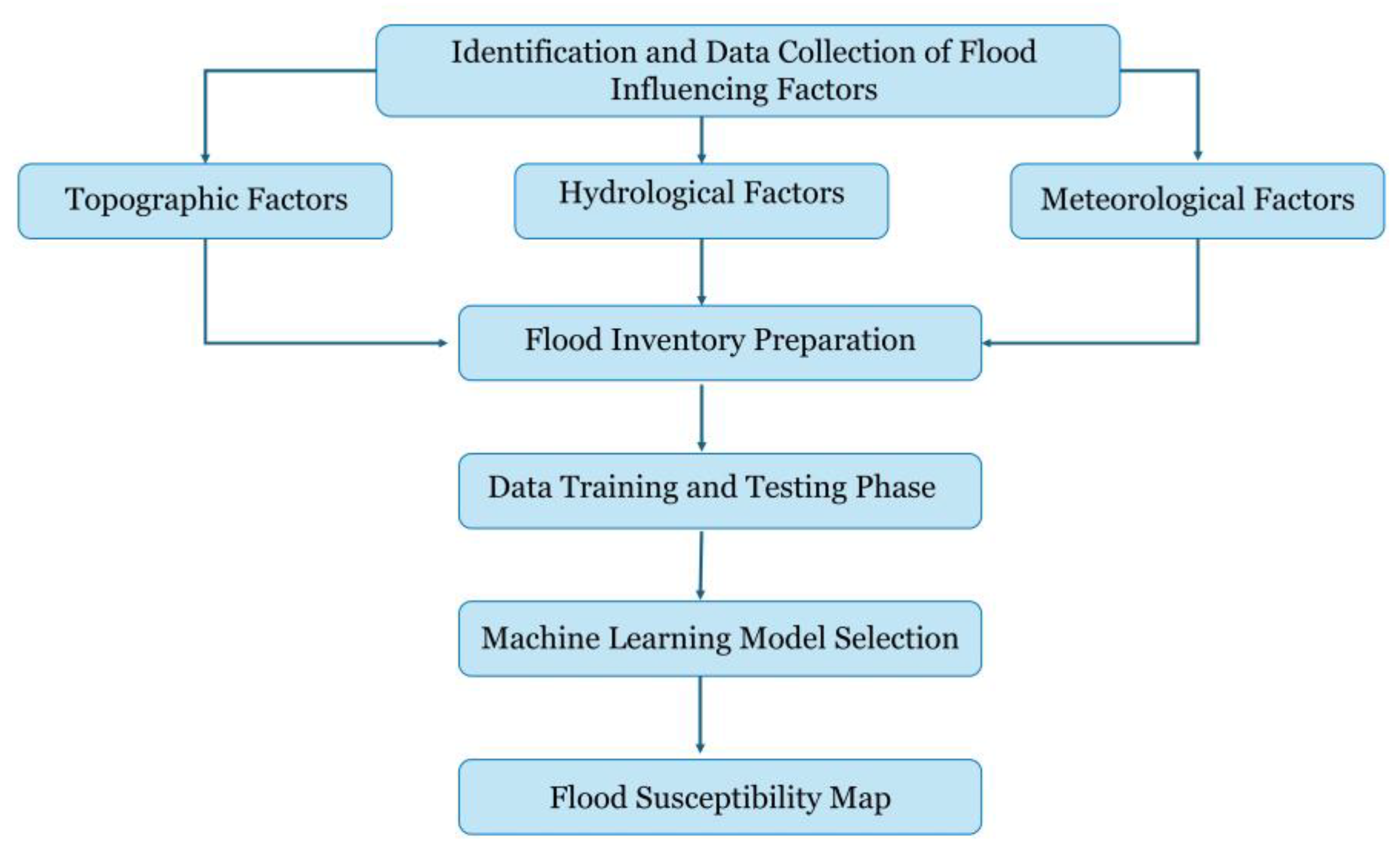
Identification of flood-influencing factors is vital for accurate flood risk forecasting and susceptibility mapping, which is often complicated by the variability in terrain, hydrological behavior, and meteorological conditions [32]. To address this challenge, the present study categorizes the selected factors into three primary groups: topographical, hydrological, and meteorological. Table 1 presents the data used in this study to identify these factors, which were processed following the methodology shown in Figure 2.
Key topographical factors such as slope, aspect, profile curvature, and tangential curvature, which describe how landscape elements affect flooding, were derived from the Digital Elevation Model (DEM) using QGIS 3.22.0 [22,25,33]. Slope, which reflects the rate of elevation change, corresponds to the first derivative of the DEM. Surface curvature, the second derivative of the DEM, affects water flow. Specifically, profile curvature influences the acceleration or deceleration of flow along the slope, while tangential curvature governs the convergence or divergence of flow across the slope, thereby affecting water accumulation [34].
Meteorological factors, particularly precipitation, play a significant role in flood risk. To capture this influence, 8 years (2015–2022) of rainfall data were gathered and interpolated using the Inverse Distance Weighted (IDW) method to generate a continuous rainfall dataset [22,26,35]. The DEM was processed using QGIS 3.22.0 to derive hydrological variables such as flow concentration, peak stream flow, and flow velocity [25]. Discharge and rainfall data were available at only two stations within the study area; therefore, Inverse Distance Weighted (IDW) interpolation was applied to estimate values across the entire region [22,26]. River proximity was calculated using the Euclidean distance method to represent varying flood risk, with areas closer to rivers generally facing higher susceptibility [22,25]. The spatial distribution of these factors is illustrated in Figure 3.
Pixel values corresponding to all flood conditioning factors within flood-affected areas were extracted and used to train machine learning models. To ensure balanced representation of both flooded and non-flooded areas across the study region, locations were selected using a stratified random sampling technique. The final dataset consisted of 750 points, evenly split between 375 flood-prone and 375 non-flood-prone locations, maintaining class balance for binary classification. The flood inventory was split into training (70%) and testing (30%) datasets [18,36]. Three machine learning algorithms, XGBoost, logistic regression, and bagging, were employed to classify the data. During model training, 10-fold cross-validation was employed to prevent overfitting and assess generalizability. All models were trained with a maximum of 200 iterations, enabling them to learn patterns from diverse geospatial and hydrological variables influencing flood susceptibility. Model performance was evaluated using confusion matrices, ROC curves, and AUC scores, which provide insights into the model’s discriminatory ability beyond simple accuracy [37,38]. After validation, the trained model was applied to the final dataset with appropriate column alignment. Assumptions were incorporated, and flood susceptibility classes along with probability values for each class were generated.

3.2. Machine Learning Model Selection

For this study, ensuring accurate and reliable flood susceptibility mapping required selecting suitable machine learning models that are also easy to interpret. To simplify the flood susceptibility mapping process, we employed logistic regression, XGBoost, and bagging models.
Logistic regression is a simple and effective way to assess flood risk by calculating the probability of flooding based on factors like rainfall, soil moisture, topography, land use, and distance to water bodies [39]. A key advantage of this approach is its ability to identify the most influential flood-driving factors, aiding informed decision-making. However, it assumes a linear relationship between these variables and flood risk, which may not always hold true, and it is sensitive to outliers [40]. Despite these limitations, logistic regression provides valuable insights into the primary drivers of flood risk and establishes a strong foundation for understanding flood vulnerability [38,39,41].
Bagging, specifically the random forest method, is used to improve prediction accuracy and capture complex flood patterns. It creates multiple decision trees from different data subsets and combines their outputs to produce more stable predictions [42]. This technique reduces errors and overfitting, making it especially effective when environmental variables interact in complex, nonlinear ways [43]. Although bagging requires more computational power, it provides more accurate and consistent flood forecasts. Figure 4 illustrates the schematic diagram of the logistic regression and bagging models used for flood susceptibility assessment.
XGBoost is an advanced variant of gradient boosting trees designed for high computational efficiency and accuracy. It builds decision trees sequentially, optimizing their order to reduce errors and uses regularization methods to prevent overfitting and enhance generalization. XGBoost efficiently handles large datasets via distributed computing and can automatically manage missing values, making it a powerful and flexible tool for machine learning tasks [44].

3.3. Hyperparameter Tuning (Grid SearchCV)

To improve model performance and generalization, Grid SearchCV with 5-fold cross-validation was used to systematically optimize hyperparameters for logistic regression, XGBoost, and bagging classifiers. For logistic regression, a range of regularization strengths (C) was tested to balance bias and variance, along with different solvers (liblinear, lbfgs, and saga) suitable for small-to-medium-sized datasets with an l2 penalty [45]. For XGBoost, tuning was performed on the number of weak learners (n_estimators) and the learning_rate, which determines the contribution of each learner. Lower learning rates, such as 0.00001 and 0.0001, were included to prevent overfitting and encourage gradual learning [46]. For bagging, the number of base estimators was optimized, and various sampling fractions (max_samples and max_features) were tested to evaluate how subsampling affects model variance and bias [47]. These hyperparameter selections were informed by established practices and empirical validation to guarantee robust and accurate model performance and are tabulated in Table 2.

4. Results and Discussions

4.1. Correlation Analysis of Flood Conditioning Factors

Figure 5 displays the correlation matrix heatmap, which depicts the relationship between flood occurrence (FNF) and several flood conditioning factors. Notably, elevation and distance to river (DTR) show the strongest negative correlations with FNF, at −0.50 and −0.55, respectively, suggesting that flooding is less likely in areas located at higher elevations and farther from riverbanks. The slope variable reveals a moderate negative correlation (−0.24), indicating that steeper slopes promote quicker water runoff and thus reduce flood accumulation. In contrast, rainfall exhibits only a very weak positive correlation (0.03), signifying that rainfall alone is a weak predictor of flooding in this dataset. Additionally, other terrain and flow-related factors—such as flow velocity, curvatures, and flow concentration—demonstrate minimal correlation with FNF, which suggests their direct influence on flood occurrence is limited.

4.2. Performance Metrics of Machine Learning Models

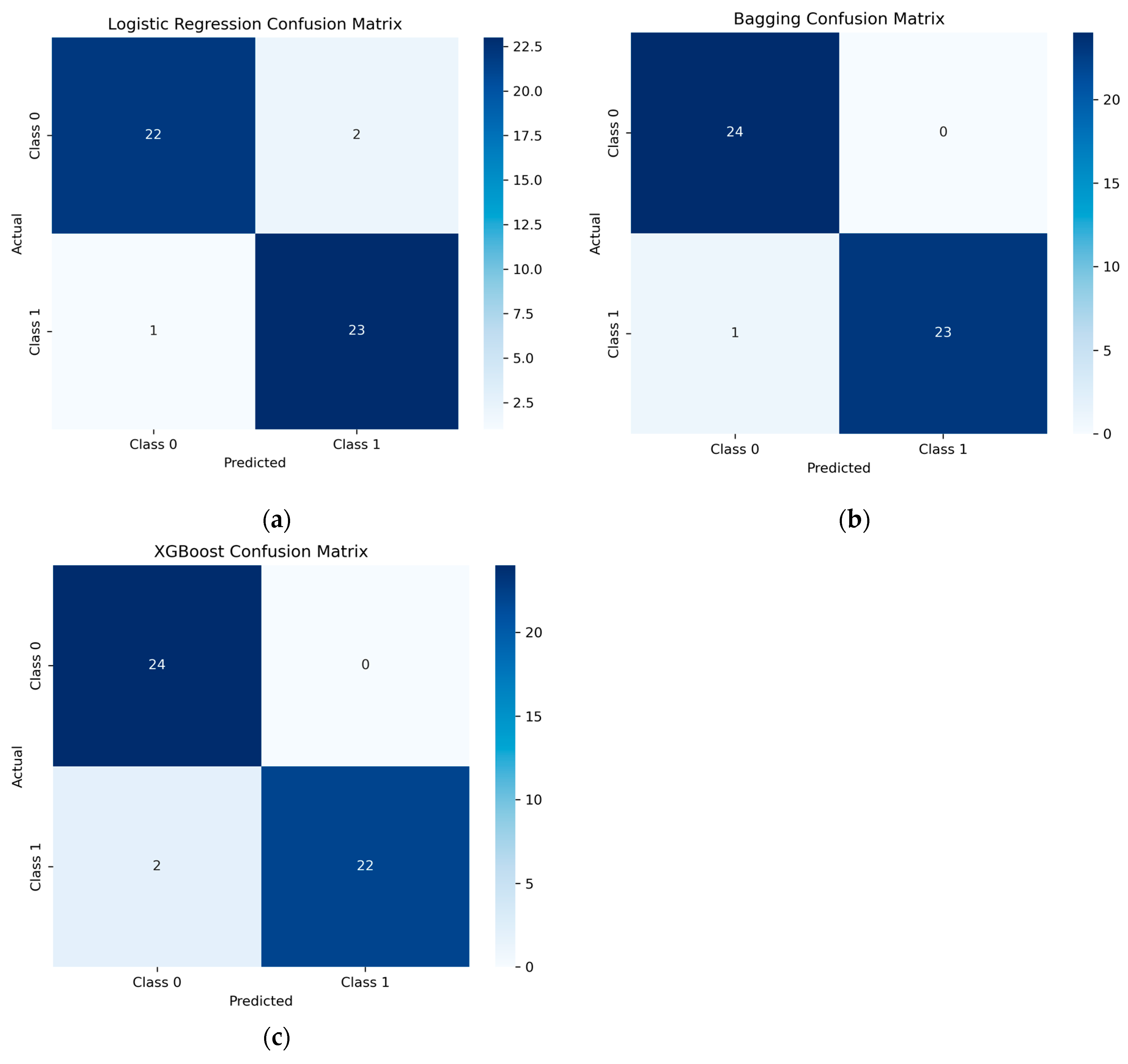
Figure 6 shows the confusion matrix analysis for all three models. Logistic regression achieved 22 true negatives, 23 true positives, 2 false positives, and 1 false negative, indicating high accuracy and perfect precision. Bagging correctly classified 23 flood-prone and 24 non-flood areas, with 1 false negative and no false positives. XGBoost correctly identified 22 flood-prone and 24 non-flood areas, with 2 false negatives and no false positives. The performance metrics for all models are presented in Table 3. While all models performed strongly, their error profiles reveal subtle trade-offs.
Four key metrics—F1-score, accuracy, precision, and recall—were used to evaluate the models. Logistic regression led with 97.92% accuracy, perfect precision (100%), and an F1-score of 0.9787. Bagging followed with 93.75% accuracy, 92% precision, and an F1-score of 0.9388. XGBoost performed strongly as well, achieving 95.83% accuracy, perfect precision, a recall of 91.67%, and an F1-score of 0.9565. All three showed similar recall around 91–96%, demonstrating effective flood risk detection.
Stratified 10-fold cross-validation confirmed logistic regression’s stable performance with minimal variance across folds, while bagging showed more fluctuation in precision, likely due to its stochastic sampling process. XGBoost also maintained consistent results, supporting its reliability. These findings highlight logistic regression’s superior stability and generalizability, vital for real-world application. From an operational standpoint, logistic regression’s flawless precision minimizes false alarms, enhancing emergency response and user trust. Bagging’s high recall makes it valuable where sensitivity is paramount, such as severe weather events or sensor-limited regions. XGBoost’s strong overall metrics and perfect precision position it as a reliable alternative, though its slightly lower recall should be considered. Logistic regression remains the most interpretable and dependable choice for most scenarios. Error analysis shows misclassifications occurred near decision boundaries or in complex terrains, suggesting that incorporating higher-resolution geographic data and real-time dynamic predictors like soil saturation or rainfall could further improve accuracy. Overall, while all models are dependable, logistic regression’s superior accuracy and faultless precision make it the best suited for practical flood risk management.

4.3. ROC Curve Interpretation

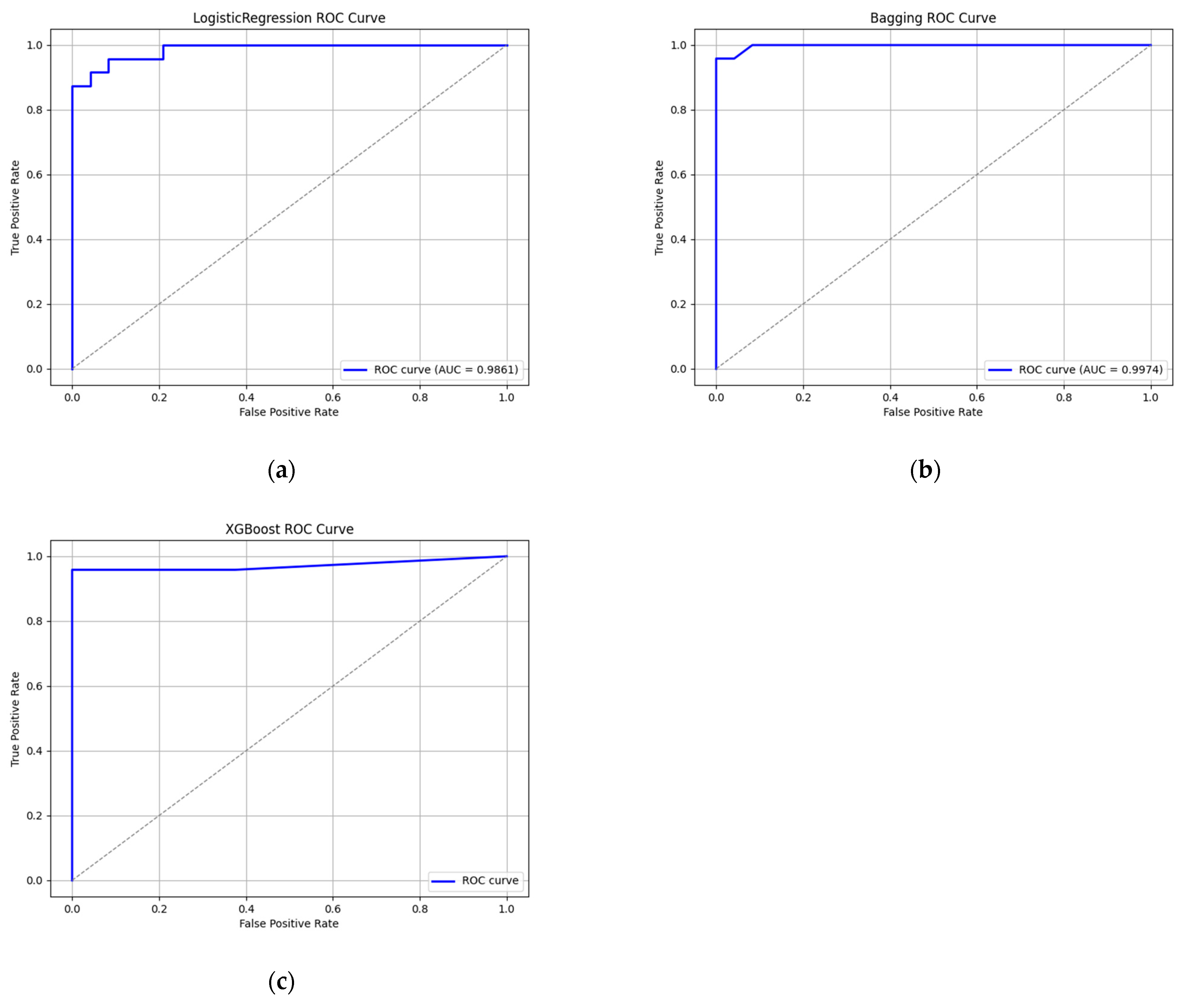
The ROC curves reveal subtle differences between models, as illustrated in Figure 7. Logistic regression attains an AUC of 0.9861 with a moderate incremental rise, while bagging’s ROC curve exhibits a steep vertical ascent, achieving a higher AUC of 0.9974. XGBoost, on the other hand, records the lowest AUC among all the models, with a value of 0.9714. Despite bagging’s superior probability ranking indicated by its AUC, logistic regression remains the preferred model for flood risk assessment due to its higher overall accuracy and perfect precision, which ensures dependable detection with fewer false alarms. Examining the ROC curve shapes further clarifies model behavior. Bagging’s curve rises sharply at low false positive rates, reflecting excellent early sensitivity—a critical trait for emergency flood detection aiming to capture as many flood events as possible. In contrast, logistic regression’s curve rises more gradually, indicating more conservative, precise classifications that prioritize certainty over sensitivity.
In flood forecasting, balancing sensitivity (recall) and specificity (precision) is vital, as both false positives and false negatives carry significant costs. While bagging’s high sensitivity reduces missed floods, it risks generating excessive false alarms, potentially undermining public trust. Logistic regression’s conservative approach minimizes false alerts but may overlook some flood events. Thus, selecting an operational classification threshold is essential and context-dependent: higher thresholds favor precision, reducing false alarms, whereas lower thresholds prioritize recall to avoid missing floods. Although bagging’s slight AUC advantage could be statistically evaluated, both models demonstrate exceptional discriminative power. However, bagging’s marginal benefit does not outweigh logistic regression’s superior accuracy, interpretability, and reliability—attributes crucial for real-world applications. Logistic regression’s straightforward probabilistic output and resilience make it ideal for early warning systems and policy applications.
Overall, logistic regression’s combination of accuracy and robustness best serves Briar Creek flood risk prediction, particularly under resource constraints and time-sensitive decision-making. Ensemble methods like Bagging may complement this by providing early-stage detection but are secondary to the consistent precision of logistic regression.

4.4. Feature Importance for Machine Learning Models

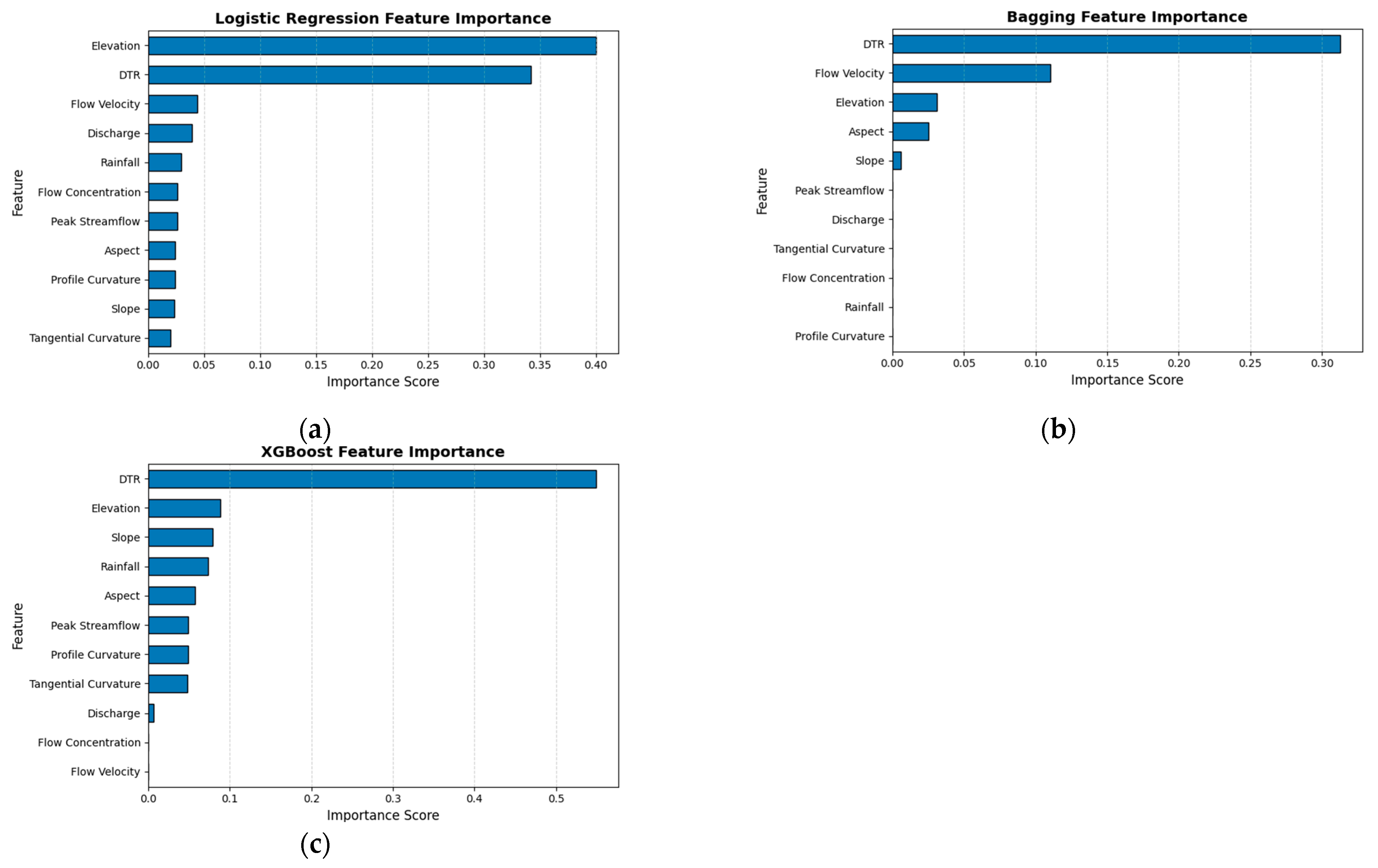
The importance of each flood conditioning factor was assessed for the logistic regression, bagging, and XGBoost models, as shown in Figure 8. This helps to understand how each model evaluates and prioritizes different factors when predicting flood-prone areas.
In the logistic regression model, elevation and distance to river (DTR) stand out as the most significant predictors. This means the model heavily depends on these two factors, recognizing that areas at lower elevations and closer to rivers are more likely to flood. Other variables like flow velocity, discharge, and rainfall also contribute to the predictions but to a lesser extent. Terrain-related features such as slope and profile curvature play a smaller role. Overall, the model follows a clear ranking, where variables with direct links to flooding are given more weight. The bagging model, on the other hand, leans heavily on DTR. It ranks far above the other factors in importance. While flow velocity and elevation are next in line, their impact is much smaller compared to DTR. Interestingly, variables that played a moderate role in the logistic regression model—like rainfall and discharge—barely influence the bagging model’s predictions. This suggests that the bagging algorithm, which relies on a combination of decision trees, mostly uses river proximity alone to make its decisions, treating other factors as less relevant. The XGBoost model tells a somewhat similar story. Like bagging, it considers DTR the most important factor by a wide margin, followed by elevation, slope, and rainfall. However, compared to bagging, XGBoost gives more weight to a broader set of variables, especially topographical and weather-related ones. Still, it assigns little importance to flow velocity and flow concentration, which logistic regression had found to be more meaningful.
Distance to river and elevation consistently rank as the top factors driving flood risk in the Briar Creek watershed. This agreement across different types of models strengthens confidence in their significance. Where the models differ is in how they treat the less dominant factors. Logistic regression takes a more balanced approach by spreading importance across multiple variables, while bagging and XGBoost focus more narrowly on one or two key predictors. These differences in how each model weighs the input data help explain why their flood risk maps show variations across the region.

4.5. Flood Risk Susceptibility Map

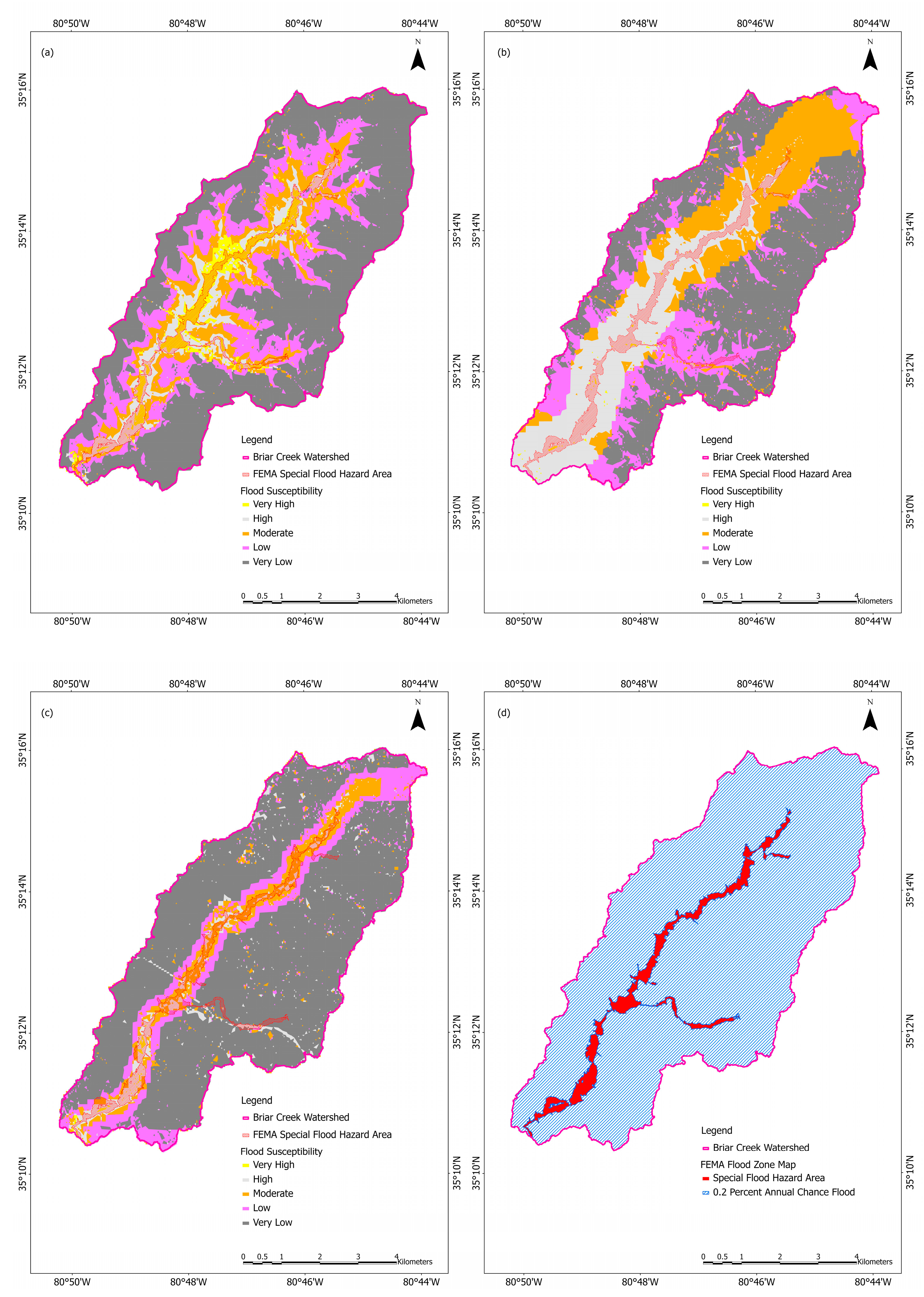
The flood susceptibility maps as shown in Figure 9 were classified into five distinct risk zones based on the probability values generated by the susceptibility models. In classification, prior probabilities reflect class distributions before observing any features and influence model behavior, especially with imbalanced data. Some models like logistic regression adjust for priors through intercepts or probability calibration (Platt scaling), while tree-based models and XGBoost respond to class imbalance via weighting or gradient scaling. After predicting probabilities, we can discretize them into five ordinal classes from very low to very high using binning. These probability values ranged from 0 to 1 and were reclassified using equal interval classification to represent varying levels of flood susceptibility. The classification scheme was divided as follows: very low risk (0.00–0.20), low risk (0.21–0.40), moderate risk (0.41–0.60), high risk (0.61–0.80), and very high risk (0.81–1.00).
The spatial distribution of flood risk classes varies across the three models, as shown in Table 4. Logistic regression classifies 5.55% of the area as very high risk, 8.66% as high risk, 12.04% as moderate risk, 21.57% as low risk, and 52.18% as very low risk, reflecting a gradual risk gradient and a cautious approach to identifying high-risk zones. Bagging assigns only 0.25% to very high risk but a substantially larger portion (22.47%) to high risk, with moderate at roughly 19%, low risk at roughly 18%, and 39.54% as very low risk, indicating a more even distribution across risk categories. XGBoost results show 0.31% very high risk, 6.37% high risk, 9.19% moderate risk, 13.85% low risk, and the largest share, 70.28%, as very low risk. Overall, logistic regression appears more conservative in delineating high-risk areas, whereas bagging emphasizes a broader high-risk zone, and XGBoost classifies most of the region at very low risk. These differences underscore each model’s distinct risk prioritization and spatial risk representation.
Spatial agreement of high-risk zones (classes 1 and 2) among logistic regression, bagging, and XGBoost is limited, as shown in Table 5. Only 1.63% of the area is consistently classified as high risk by all three. Logistic regression and bagging overlap most (5.90%), followed by bagging and XGBoost (1.97%) and logistic regression and XGBoost (1.76%). Logistic regression and XGBoost confine high-risk zones to core floodplain areas along Briar Creek, whereas bagging extends these zones into adjacent low-lying regions. All models agree on main flood pathways, but bagging’s broader high-risk areas suggest a more conservative, inclusive flood risk identification.
For the Briar Creek watershed, FEMA has designated two flood zones: AE, indicating the Special Flood Hazard Area (SFHA), and X, representing the 0.2% annual chance flood, as illustrated in Figure 9d. Table 6 compares the spatial agreement of the very-high-risk zones identified by the three models with FEMA’s SFHA classification for the Briar Creek watershed.
There is a strong overlap between FEMA’s designation of special flood hazard zones and the high-risk areas identified by the logistic regression model, with most of these zones concentrated along Briar Creek and its floodplain. Although bagging and XGBoost do not classify most of the floodplain vicinity as very-high-risk, they similarly recognize these areas as high-risk.

4.6. Limitations and Potential Directions for Future Research

In this study, spatial validation was conducted using FEMA flood hazard designations effective from February 2014. The observed overlap between high-risk zones mapped by the machine learning models and FEMA’s Special Flood Hazard Area underscores the effectiveness of ML-based flood susceptibility mapping. However, several limitations remain.
A key limitation is the lack of spatial validation against observed flow or flood extent from actual flood events in the Briar Creek watershed, which restricts the ability to fully assess model accuracy in real-world conditions. Furthermore, sparse gauge coverage could contribute to interpolation bias, affecting model reliability. Ensemble methods like Bagging and XGBoost, despite their robustness, may suffer from spatial selectivity and require careful hyperparameter tuning to avoid overfitting local patterns.
Regarding prediction accuracy and robustness, the logistic regression model outperformed others, indicating that linear relationships may sufficiently capture the primary drivers of flooding in this watershed. However, hydrological processes are often characterized by nonlinear thresholds and spatial heterogeneity, which ensemble methods such as XGBoost and bagging are better suited to address [48]. These nonlinear approaches provide a flexible framework capable of adapting to complex hydrological regimes while maintaining robustness—an advantage when scaling to diverse flood-prone environments [49]. Nonetheless, this study’s reliance on static input variables, including the absence of dynamic real-time predictors like soil moisture and rainfall intensity, may constrain the predictive power of all models, particularly those like XGBoost and bagging that depend on capturing intricate interactions. Incorporating dynamic, high-resolution predictors would likely enhance model performance and reliability in future applications.

5. Conclusions

This study developed and evaluated machine learning models—logistic regression, bagging, and XGBoost—for flood susceptibility mapping in the urbanized Briar Creek watershed using hydrological, topographical, and meteorological data. Logistic regression was identified as the most accurate machine learning model for flood susceptibility mapping in the study area. Among the flood conditioning factors, elevation and distance to river were the most influential in determining flood risk. Using this ML model, the flood risk zones were classified into five categories, with 5.55% of the area mapped as very high risk, 8.66% as high risk, 12.04% as moderate risk, 21.56% as low risk, and 52.20% as very low risk. Notably, logistic regression’s very-high-risk classification closely aligned with FEMA’s Special Flood Hazard Area designation, which covers 5.29% of the Briar Creek floodplain. This strong correspondence validates the model’s effectiveness and suggests its suitability as a valuable tool for planners and emergency managers to guide flood mitigation efforts and reduce potential losses in future flood events.
Furthermore, this work offers a reproducible framework for applying ML in similar urban watersheds. Future improvements could include real-time sensor integration, higher-resolution inputs, and incorporation of socioeconomic factors to enhance predictive accuracy and support urban resilience efforts.

Author Contributions

Conceptualization, A.K.; formal analysis, S.S., investigation, S.R., N.B., D.D. and S.S.; software, A.K. and D.D.; supervision, A.K.; writing—initial draft preparation, S.R., S.S., N.B. and R.S.; writing—review and editing, A.K., S.R. and R.S. All authors have read and agreed to the published version of the manuscript.

Funding

This research received no external funding.

Data Availability Statement

The data used in this study are available upon request from the corresponding author.

Acknowledgments

The authors would like to thank the reviewers for their valuable suggestions. The authors acknowledge the support of Southern Illinois University and Carbondale’s Vice-Chancellor for Research. The research, simulation, and analysis were performed with open-source software and datasets.

Conflicts of Interest

The authors declare no conflicts of interest.

References

  1. Islam, M.Z.; Wang, C. Cost of High-Level Flooding as a Consequence of Climate Change Driver?: A Case Study of China’s Flood-Prone Regions. Ecol. Indic. 2024, 160, 111944. [Google Scholar] [CrossRef]
  2. Dahal, D.; Shrestha, S.; Poudel, B.; Banjara, M.; Kalra, A. The Role of Reclaimed Water in Urban Flood Management: Public Perception and Acceptance. Earth Sci. Res. 2025, 14, 1. [Google Scholar] [CrossRef]
  3. Teku, D.; Eshetu, S. Impact of Climatic Variabilities and Extreme Incidences on the Physical Environment, Public Health, and People’s Livelihoods in Ethiopia. Front. Clim. 2024, 6, 1435138. [Google Scholar] [CrossRef]
  4. Ruan, X.; Sun, H.; Shou, W.; Wang, J. The Impact of Climate Change and Urbanization on Compound Flood Risks in Coastal Areas: A Comprehensive Review of Methods. Appl. Sci. 2024, 14, 10019. [Google Scholar] [CrossRef]
  5. Mucherera, B.; Spiegel, S. Forced Displacement: Critical Lessons in the Protracted Aftermath of a Flood Disaster. GeoJournal 2022, 87, 3855–3875. [Google Scholar] [CrossRef]
  6. Nguyen, H.N.; Fukuda, H.; Nguyen, M.N. Assessment of the Susceptibility of Urban Flooding Using GIS with an Analytical Hierarchy Process in Hanoi, Vietnam. Sustainability 2024, 16, 3934. [Google Scholar] [CrossRef]
  7. Swain, K.C.; Singha, C.; Nayak, L. Flood Susceptibility Mapping through the GIS-AHP Technique Using the Cloud. ISPRS Int. J. Geo-Inf. 2020, 9, 720. [Google Scholar] [CrossRef]
  8. Hammami, S.; Zouhri, L.; Souissi, D.; Souei, A.; Zghibi, A.; Marzougui, A.; Dlala, M. Application of the GIS Based Multi-Criteria Decision Analysis and Analytical Hierarchy Process (AHP) in the Flood Susceptibility Mapping (Tunisia). Arab. J. Geosci. 2019, 12, 653. [Google Scholar] [CrossRef]
  9. Fletcher, T.D.; Andrieu, H.; Hamel, P. Understanding, Management and Modelling of Urban Hydrology and Its Consequences for Receiving Waters: A State of the Art. Adv. Water Resour. 2013, 51, 261–279. [Google Scholar] [CrossRef]
  10. Tehrany, M.S.; Pradhan, B.; Jebur, M.N. Spatial Prediction of Flood Susceptible Areas Using Rule Based Decision Tree (DT) and a Novel Ensemble Bivariate and Multivariate Statistical Models in GIS. J. Hydrol. 2013, 504, 69–79. [Google Scholar] [CrossRef]
  11. Dahal, D.; Magar, B.A.; Aryal, A.; Poudel, B.; Banjara, M.; Kalra, A. Analyzing Climate Dynamics and Developing Machine Learning Models for Flood Prediction in Sacramento, California. Hydroecol. Eng. 2024, 1, 10003. [Google Scholar] [CrossRef]
  12. Jahanbani, M.; Vahidnia, M.H.; Aghamohammadi, H.; Azizi, Z. Flood Susceptibility Mapping through Geoinformatics and Ensemble Learning Methods, with an Emphasis on the AdaBoost-Decision Tree Algorithm, in Mazandaran, Iran. Earth Sci. Inform. 2024, 17, 1433–1457. [Google Scholar] [CrossRef]
  13. Zahraoui, Y.; Korõtko, T.; Rosin, A.; Mekhilef, S.; Seyedmahmoudian, M.; Stojcevski, A.; Alhamrouni, I. AI Applications to Enhance Resilience in Power Systems and Microgrids—A Review. Sustainability 2024, 16, 4959. [Google Scholar] [CrossRef]
  14. Sadkou, S.; Artigue, G.; Fréalle, N.; Ayral, P.; Pistre, S.; Sauvagnargues, S.; Johannet, A. A Review of Flash-floods Management: From Hydrological Modeling to Crisis Management. J. Flood Risk Manag. 2024, 17, e12999. [Google Scholar] [CrossRef]
  15. Mosavi, A.; Ozturk, P.; Chau, K. Flood Prediction Using Machine Learning Models: Literature Review. Water 2018, 10, 1536. [Google Scholar] [CrossRef]
  16. Tehrany, M.S.; Pradhan, B.; Mansor, S.; Ahmad, N. Flood Susceptibility Assessment Using GIS-Based Support Vector Machine Model with Different Kernel Types. CATENA 2015, 125, 91–101. [Google Scholar] [CrossRef]
  17. Shahabi, H.; Shirzadi, A.; Ghaderi, K.; Omidvar, E.; Al-Ansari, N.; Clague, J.J.; Geertsema, M.; Khosravi, K.; Amini, A.; Bahrami, S.; et al. Flood Detection and Susceptibility Mapping Using Sentinel-1 Remote Sensing Data and a Machine Learning Approach: Hybrid Intelligence of Bagging Ensemble Based on K-Nearest Neighbor Classifier. Remote Sens. 2020, 12, 266. [Google Scholar] [CrossRef]
  18. Hoang, D.-V.; Liou, Y.-A. Elevating Flash Flood Prediction Accuracy: A Synergistic Approach with PSO and GA Optimization. Nat. Hazards Earth Syst. Sci. 2024, 2024, 1–26. [Google Scholar]
  19. Costache, R.; Tien Bui, D. Spatial Prediction of Flood Potential Using New Ensembles of Bivariate Statistics and Artificial Intelligence: A Case Study at the Putna River Catchment of Romania. Sci. Total Environ. 2019, 691, 1098–1118. [Google Scholar] [CrossRef]
  20. Oliva, A.; Olcina, J. Historical Floods and Territorial Planning: Lessons Learned and Opportunities Lost after the Santa Teresa Flood (1879) in the Segura Basin (Spain). Land 2023, 13, 28. [Google Scholar] [CrossRef]
  21. Gizzi, F.T.; Bovolin, V.; Villani, P.; Potenza, M.R.; Voria, S.; Amodio, A.M. Rewinding the Tape: Documentary Heritage to (Re)Discover “Lost” Natural Hazards—Evidence and Inferences from Southern Italy. Sustainability 2024, 16, 2789. [Google Scholar] [CrossRef]
  22. Shrestha, S.; Dahal, D.; Poudel, B.; Banjara, M.; Kalra, A. Flood Susceptibility Analysis with Integrated Geographic Information System and Analytical Hierarchy Process: A Multi-Criteria Framework for Risk Assessment and Mitigation. Water 2025, 17, 937. [Google Scholar] [CrossRef]
  23. Kalra, A.; Shrestha, S.; Dahal, D.; Banjara, M.; Paudel, B.; Gupta, R. Assessing the Performance of HEC-HMS and SWMM Models for Rainfall–Runoff Simulation for Urban Watershed. In Proceedings of the World Environmental and Water Resources Congress 2025, Anchorage, Alaska, 18–21 May 2025; pp. 1230–1242. [Google Scholar] [CrossRef]
  24. Buchholz, T.A.; Madary, D.A.; Bork, D.; Younos, T. Stream restoration in urban environments: Concept, design principles, and case studies of stream daylighting. In Sustainable Water Management in Urban Environments; Younos, T., Parece, T.E., Eds.; Springer International Publishing: Cham, Switzerland, 2016; pp. 121–165. ISBN 978-3-319-29337-0. [Google Scholar]
  25. Shrestha, B.; Rajbhandari, E.; Kayastha, R.B.; Shrestha, S.; Dahal, D. Assessing Flood Susceptibility and Frequency Analysis in Himalayan River Basins: A GIS-Based Multi-Criteria Approach. Kathmandu Univ. J. Sci. Eng. Technol. 2025, 19. [Google Scholar] [CrossRef]
  26. Vojtek, M.; Vojteková, J. Flood Susceptibility Mapping on a National Scale in Slovakia Using the Analytical Hierarchy Process. Water 2019, 11, 364. [Google Scholar] [CrossRef]
  27. Chen, Y.; Liu, R.; Barrett, D.; Gao, L.; Zhou, M.; Renzullo, L.; Emelyanova, I. A Spatial Assessment Framework for Evaluating Flood Risk under Extreme Climates. Sci. Total Environ. 2015, 538, 512–523. [Google Scholar] [CrossRef]
  28. Thomson, H.; Zeff, H.B.; Kleiman, R.; Sebastian, A.; Characklis, G.W. Systemic Financial Risk Arising From Residential Flood Losses. Earth’s Future 2023, 11, e2022EF003206. [Google Scholar] [CrossRef]
  29. Mogollón, B.; Frimpong, E.A.; Hoegh, A.B.; Angermeier, P.L. Recent Changes in Stream Flashiness and Flooding, and Effects of Flood Management in North Carolina and Virginia. JAWRA J. Am. Water Resour. Assoc. 2016, 52, 561–577. [Google Scholar] [CrossRef]
  30. National Risk Index. Available online: https://hazards.fema.gov/nri/ (accessed on 7 May 2025).
  31. Zhou, Z.; Smith, J.A.; Yang, L.; Baeck, M.L.; Chaney, M.; Ten Veldhuis, M.; Deng, H.; Liu, S. The Complexities of Urban Flood Response: Flood Frequency Analyses for the Charlotte Metropolitan Region. Water Resour. Res. 2017, 53, 7401–7425. [Google Scholar] [CrossRef]
  32. Kaya, C.M.; Derin, L. Parameters and Methods Used in Flood Susceptibility Mapping: A Review. J. Water Clim. Chang. 2023, 14, 1935–1960. [Google Scholar] [CrossRef]
  33. Lee, S.; Rezaie, F. Data Used for GIS-Based Flood Susceptibility Mapping. GEO DATA 2022, 4, 1–15. [Google Scholar] [CrossRef]
  34. Alkhasawneh, M.S.; Ngah, U.K.; Tay, L.T.; Mat Isa, N.A.; Al-batah, M.S. Determination of Important Topographic Factors for Landslide Mapping Analysis Using MLP Network. Sci. World J. 2013, 2013, 415023. [Google Scholar] [CrossRef]
  35. Yariyan, P.; Avand, M.; Abbaspour, R.A.; Torabi Haghighi, A.; Costache, R.; Ghorbanzadeh, O.; Janizadeh, S.; Blaschke, T. Flood Susceptibility Mapping Using an Improved Analytic Network Process with Statistical Models. Geomat. Nat. Hazards Risk 2020, 11, 2282–2314. [Google Scholar] [CrossRef]
  36. Avand, M.; Moradi, H.; Lasboyee, M.R. Using Machine Learning Models, Remote Sensing, and GIS to Investigate the Effects of Changing Climates and Land Uses on Flood Probability. J. Hydrol. 2021, 595, 125663. [Google Scholar] [CrossRef]
  37. El-Haddad, B.A.; Youssef, A.M.; Pourghasemi, H.R.; Pradhan, B.; El-Shater, A.-H.; El-Khashab, M.H. Flood Susceptibility Prediction Using Four Machine Learning Techniques and Comparison of Their Performance at Wadi Qena Basin, Egypt. Nat. Hazards 2021, 105, 83–114. [Google Scholar] [CrossRef]
  38. Lee, J.-Y.; Kim, J.-S. Detecting Areas Vulnerable to Flooding Using Hydrological-Topographic Factors and Logistic Regression. Appl. Sci. 2021, 11, 5652. [Google Scholar] [CrossRef]
  39. El-Rawy, M.; Elsadek, W.M.; De Smedt, F. Flash Flood Susceptibility Mapping in Sinai, Egypt Using Hydromorphic Data, Principal Component Analysis and Logistic Regression. Water 2022, 14, 2434. [Google Scholar] [CrossRef]
  40. Kim, Y.-O.; Seo, S.B.; Jang, O.-J. Flood Risk Assessment Using Regional Regression Analysis. Nat. Hazards 2012, 63, 1203–1217. [Google Scholar] [CrossRef]
  41. Cao, Y.; Jia, H.; Xiong, J.; Cheng, W.; Li, K.; Pang, Q.; Yong, Z. Flash Flood Susceptibility Assessment Based on Geodetector, Certainty Factor, and Logistic Regression Analyses in Fujian Province, China. ISPRS Int. J. Geo-Inf. 2020, 9, 748. [Google Scholar] [CrossRef]
  42. Yariyan, P.; Janizadeh, S.; Van Phong, T.; Nguyen, H.D.; Costache, R.; Van Le, H.; Pham, B.T.; Pradhan, B.; Tiefenbacher, J.P. Improvement of Best First Decision Trees Using Bagging and Dagging Ensembles for Flood Probability Mapping. Water Resour. Manag. 2020, 34, 3037–3053. [Google Scholar] [CrossRef]
  43. Zanotti, C.; Rotiroti, M.; Sterlacchini, S.; Cappellini, G.; Fumagalli, L.; Stefania, G.A.; Nannucci, M.S.; Leoni, B.; Bonomi, T. Choosing between Linear and Nonlinear Models and Avoiding Overfitting for Short and Long Term Groundwater Level Forecasting in a Linear System. J. Hydrol. 2019, 578, 124015. [Google Scholar] [CrossRef]
  44. Ren, H.; Pang, B.; Bai, P.; Zhao, G.; Liu, S.; Liu, Y.; Li, M. Flood Susceptibility Assessment with Random Sampling Strategy in Ensemble Learning (RF and XGBoost). Remote Sens. 2024, 16, 320. [Google Scholar] [CrossRef]
  45. Friedman, J.H.; Hastie, T.; Tibshirani, R. Regularization Paths for Generalized Linear Models via Coordinate Descent. J. Stat. Softw. 2010, 33, 1–22. [Google Scholar] [CrossRef]
  46. Freund, Y.; Schapire, R.E. A Decision-Theoretic Generalization of On-Line Learning and an Application to Boosting. J. Comput. Syst. Sci. 1997, 55, 119–139. [Google Scholar] [CrossRef]
  47. Breiman, L. Bagging Predictors. Mach. Learn. 1996, 24, 123–140. [Google Scholar] [CrossRef]
  48. Beven, K.J. Rainfall-Runoff Modelling: The Primer; John Wiley & Sons: Hoboken, NJ, USA, 2012; ISBN 978-0-470-71459-1. [Google Scholar]
  49. Zounemat-Kermani, M.; Batelaan, O.; Fadaee, M.; Hinkelmann, R. Ensemble Machine Learning Paradigms in Hydrology: A Review. J. Hydrol. 2021, 598, 126266. [Google Scholar] [CrossRef]
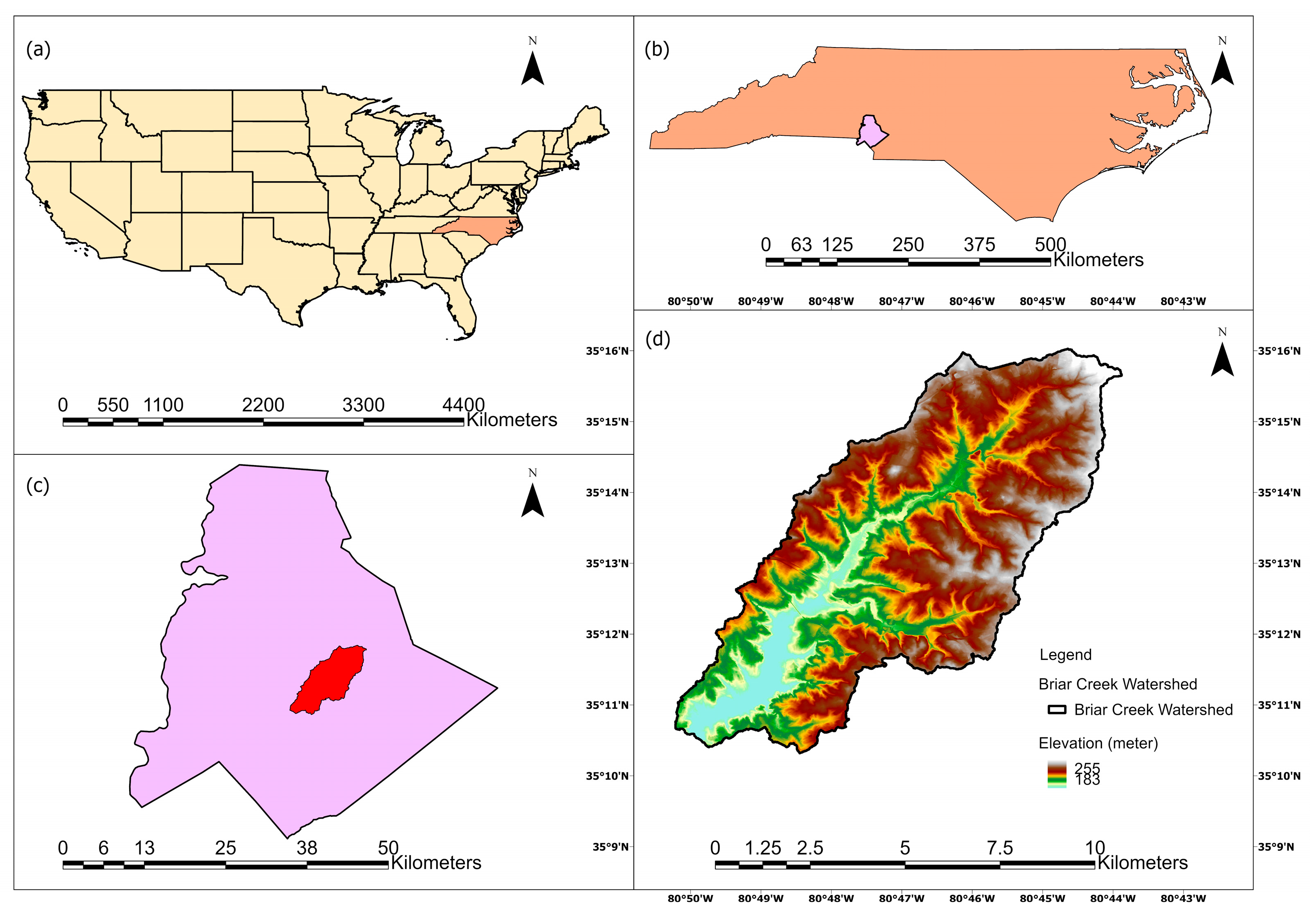
Figure 1. (a) Map of contiguous USA showing North Carolina state; (b) map of North Carolina showing Mecklenburg County; (c) map of Mecklenburg County showing Briar Creek watershed; (d) Digital Elevation Model (DEM) of Briar Creek watershed.
Geographies 05 00043 g001
Figure 2. Flowchart for flood risk susceptibility maps formulation.
Geographies 05 00043 g002
Figure 3. The spatial distribution of key flood-influencing factors, including (a) flow velocity; (b) flow concentration; (c) discharge; (d) rainfall; (e) distance to river; (f) elevation; (g) aspect; (h) slope; (i) profile curvature; (j) tangential curvature; (k) peak streamflow.
Geographies 05 00043 g003
Figure 4. (a) Schematic diagram of the logistic regression model architecture used for flood susceptibility assessment. X1, X2, and Xm represent sets of predictor features; W1, W2, and Wm represent corresponding weights; b represents the bias term; ∑ represents the calculated weighted sum of inputs plus bias; χ represents the probability value; and t assigns this probability to a discrete flood risk category. (b) Schematic diagram of the bagging model architecture used for flood susceptibility assessment.
Geographies 05 00043 g004
Figure 5. Heatmap showing the correlation matrix among various hydrological and topographical variables.
Geographies 05 00043 g005
Figure 6. Confusion matrix for (a) logistic regression; (b) bagging classifiers; (c) XGBoost.
Geographies 05 00043 g006
Figure 7. ROC Curve for (a) logistic regression; (b) bagging; (c) XGBoost models.
Geographies 05 00043 g007
Figure 8. Feature Importance for (a) logistic regression; (b) bagging; (c) XGBoost models.
Geographies 05 00043 g008
Figure 9. Flood susceptibility map based on (a) logistic regression; (b) bagging; (c) XGBoost; (d) FEMA flood zone map.
Geographies 05 00043 g009
Table 1. Overview of input data used in flood susceptibility mapping.
Data TypeSourceTemporal Coverage
Digital Elevation Model
(1 m)
National Map Viewer—U.S. Geological Survey 10 October 2024
(Published Date)
Land Use/Land Cover
(30 m × 30 m)
Multi-Resolution Land Characteristics Consortium 2019
Precipitation
(mm, 5 min interval)
National Water Information System (NWIS)1 January 2015–31 December 2022
Streamflow
(m3/s, 5 min interval)
NWIS1 January 2015–31 December 2022
Soil DataNRCS Geospatial Data Gateway22 October 2024
(Published Date)
Table 2. Overview of hyperparameter tuning for different ML models.
ModelHyperparameterValues Considered
Logistic RegressionRegularization Strength (C)
Penalty
Solver
0.01, 0.1, 1, 10
12
liblinear, lbfgs, saga
Baggingn_estimator
max_samples
max_features
50, 100, 150
0.5, 0.75, 1.0
0.5, 0.75, 1.0
XGBoostn_estimators
learning_rate
50, 100, 150
0.00001, 0.0001, 0.01, 0.1
Table 3. Performance metrics of ML models used for flood susceptibility classification.
ModelAccuracyPrecisionRecallF1 Score
Logistic Regression0.979210.95830.9787
Bagging0.93750.920.95830.9388
XGBoost0.958310.91670.9565
Table 4. Flood risk categorization results for bagging and logistic regression models.
ModelVery High
Risk (%)
High Risk
(%)
Moderate
Risk (%)
Low Risk
(%)
Very Low
Risk (%)
Logistic Regression5.558.6612.0421.5652.20
Bagging0.2522.4719.2318.5039.55
XGBoost0.316.379.1913.8570.28
Table 5. Comparison of high-risk area predictions and agreement levels across three models.
Agreement Between ModelsOverlapping High-Risk (%)
All Models1.63
Logistic Regression and Bagging5.90
Logistic Regression and XGBoost1.76
Bagging and XGBoost1.97
Table 6. Comparison between very high-risk zones from ML models and FEMA designation.
ModelsVery High Risk (%)
FEMA’s Classification5.29
Logistic Regression 5.55
Bagging0.25
XGBoost0.31
Disclaimer/Publisher’s Note: The statements, opinions and data contained in all publications are solely those of the individual author(s) and contributor(s) and not of MDPI and/or the editor(s). MDPI and/or the editor(s) disclaim responsibility for any injury to people or property resulting from any ideas, methods, instructions or products referred to in the content.