
Enhanced Forecasting of Groundwater Level Incorporating an Exogenous Variable: Evaluating Conventional Multivariate Time Series and Artificial Neural Network Models

 ,
,  and
and
Abstract
1. Introduction
2. The Study Area
2.1. Aquifer Characteristics
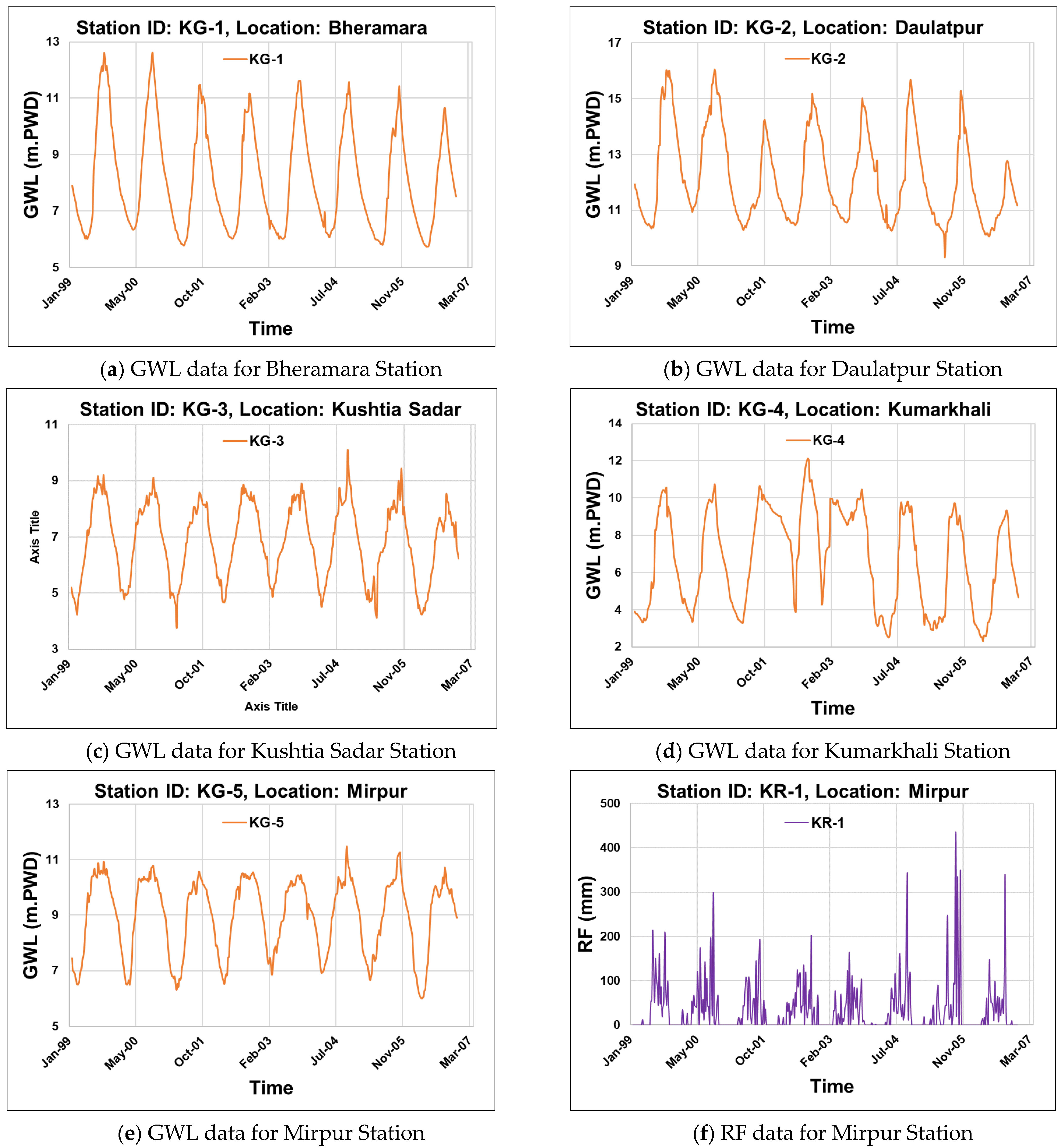
2.2. Data Description
3. Methodology
3.1. Advantages of ANN Models
3.2. Prediction Approaches of the Models
3.3. Development Strategy of ANN Models
3.3.1. Dataset Preparation
3.3.2. ANN Model Architecture and Model Training
3.4. ARIMA-Based Model Development
3.4.1. Mathematical Expression of the ARIMA Model
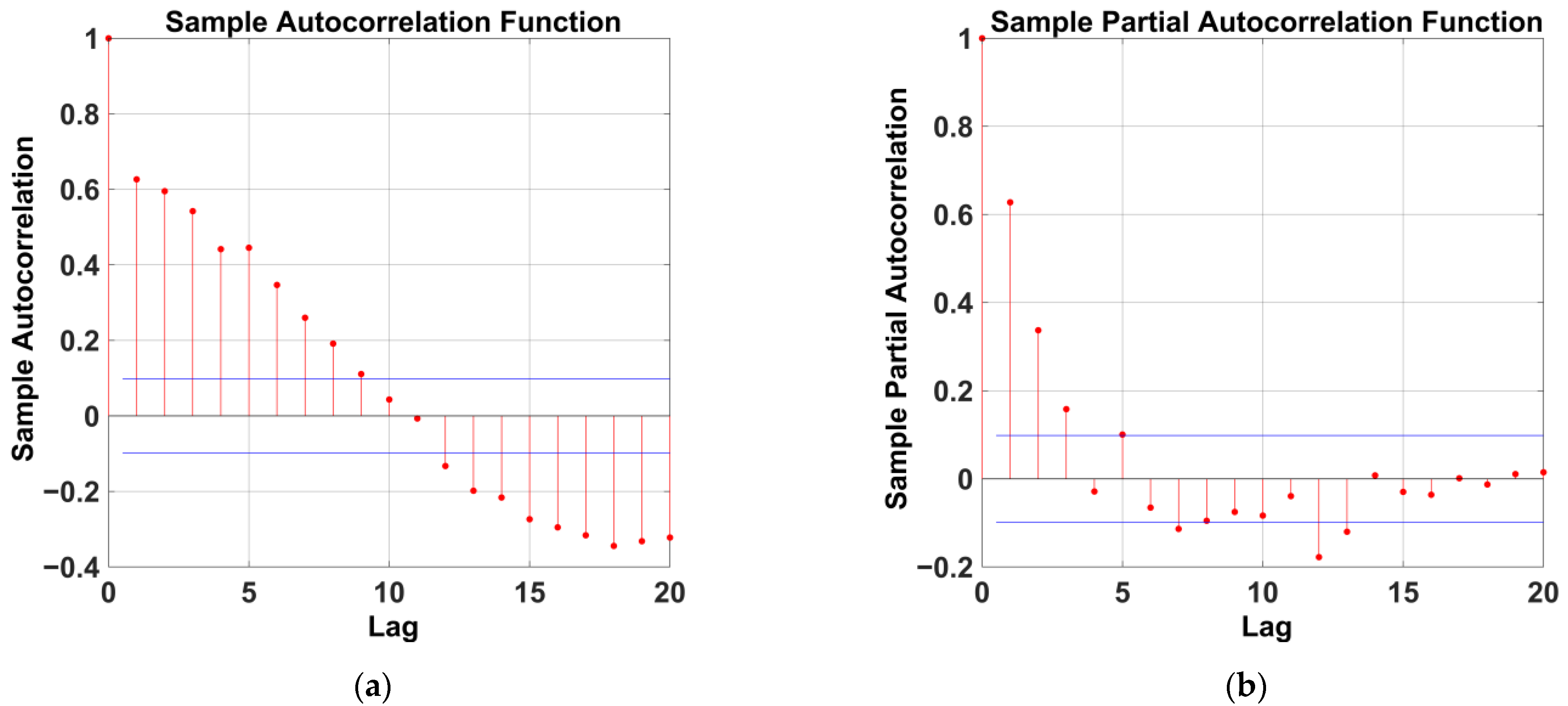
3.4.2. Model Identification
3.5. Model Evaluation Criteria
4. Results and Discussion
4.1. Performance of ANN Models
4.2. Performance Overview of Different ANN Models in the Building Stages
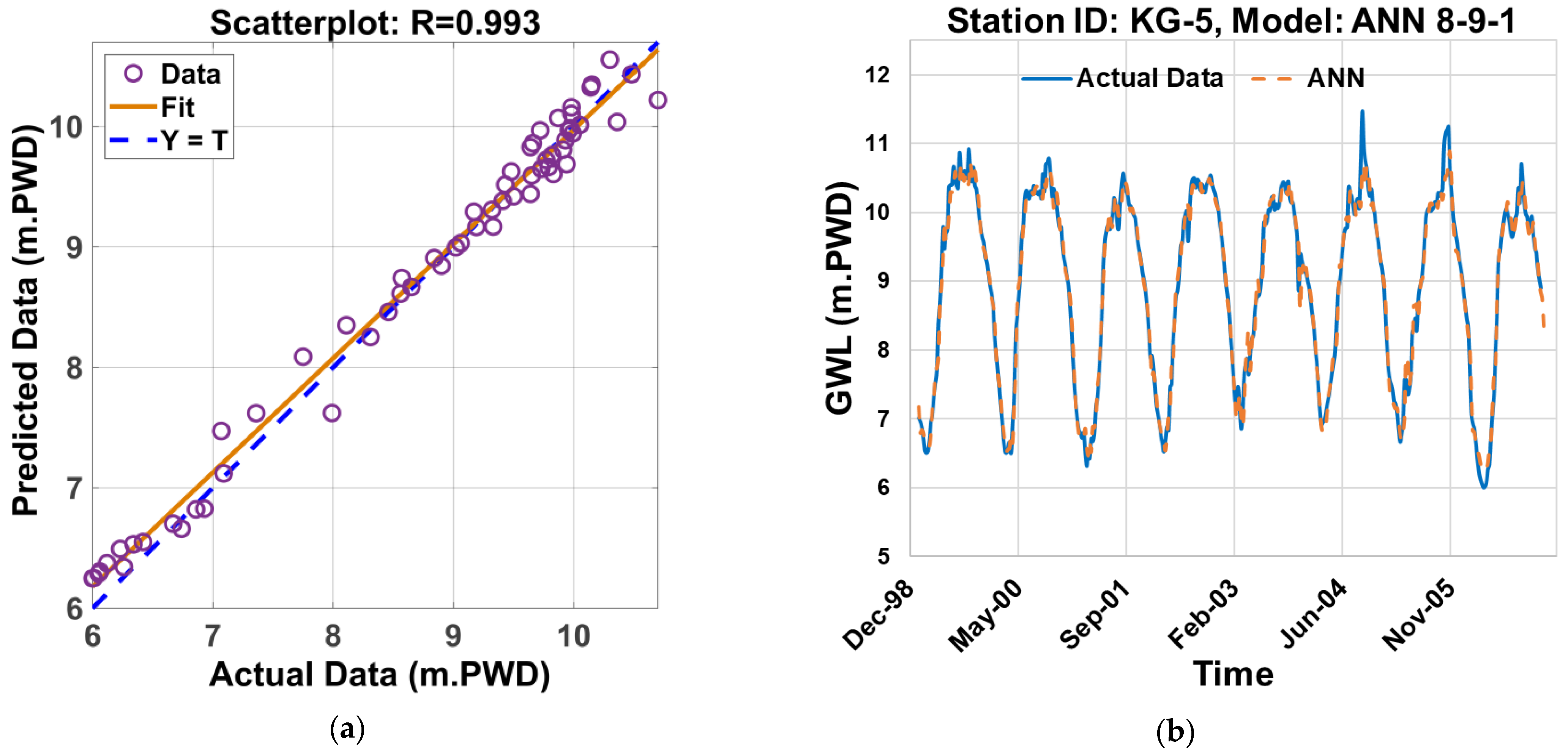
4.3. Graphical Evaluation of the Selected Performances of the ANN Model
4.4. Performances of ARIMA-Based Models
4.5. Performance Overview of Different ARIMA Models
4.6. Evaluation of the Parameters of the ARIMA Models
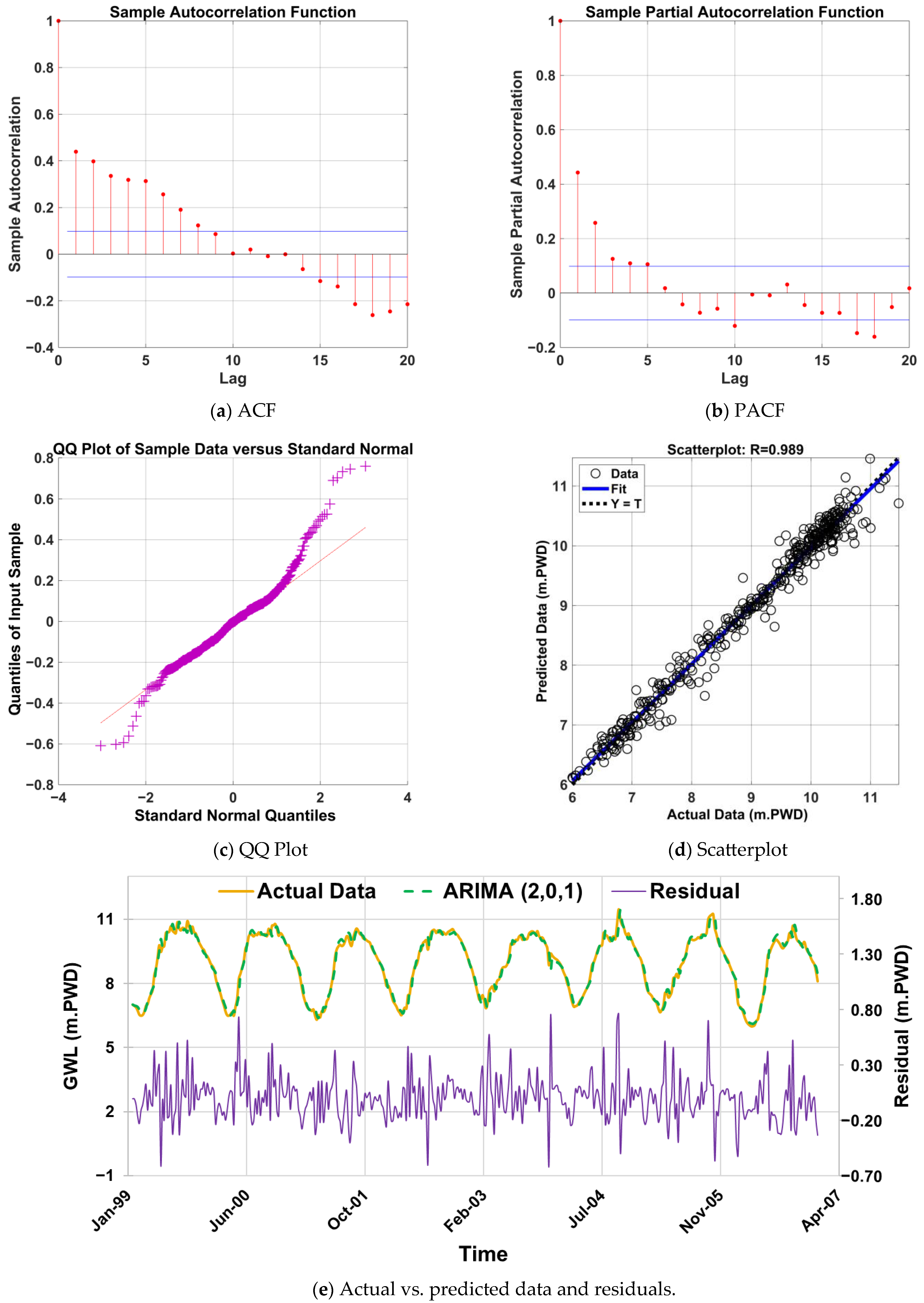
4.7. Graphical Evaluation of the Selected ARIMA Model Performances
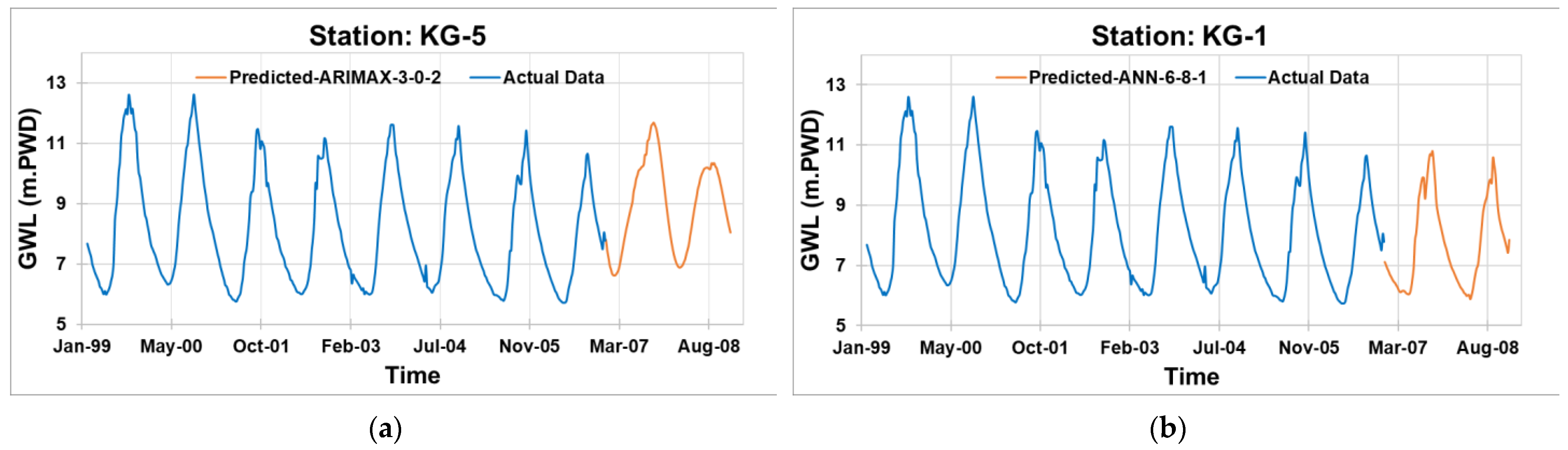
4.8. Forecasting of GWL
4.9. Relative Improvement in the Performances of Models and Comparison of the Best Models
4.9.1. Assessing the Efficiency of Models Relative to ANN
4.9.2. Assessing the Efficiency of Models Relative to the ARIMA-Based Model
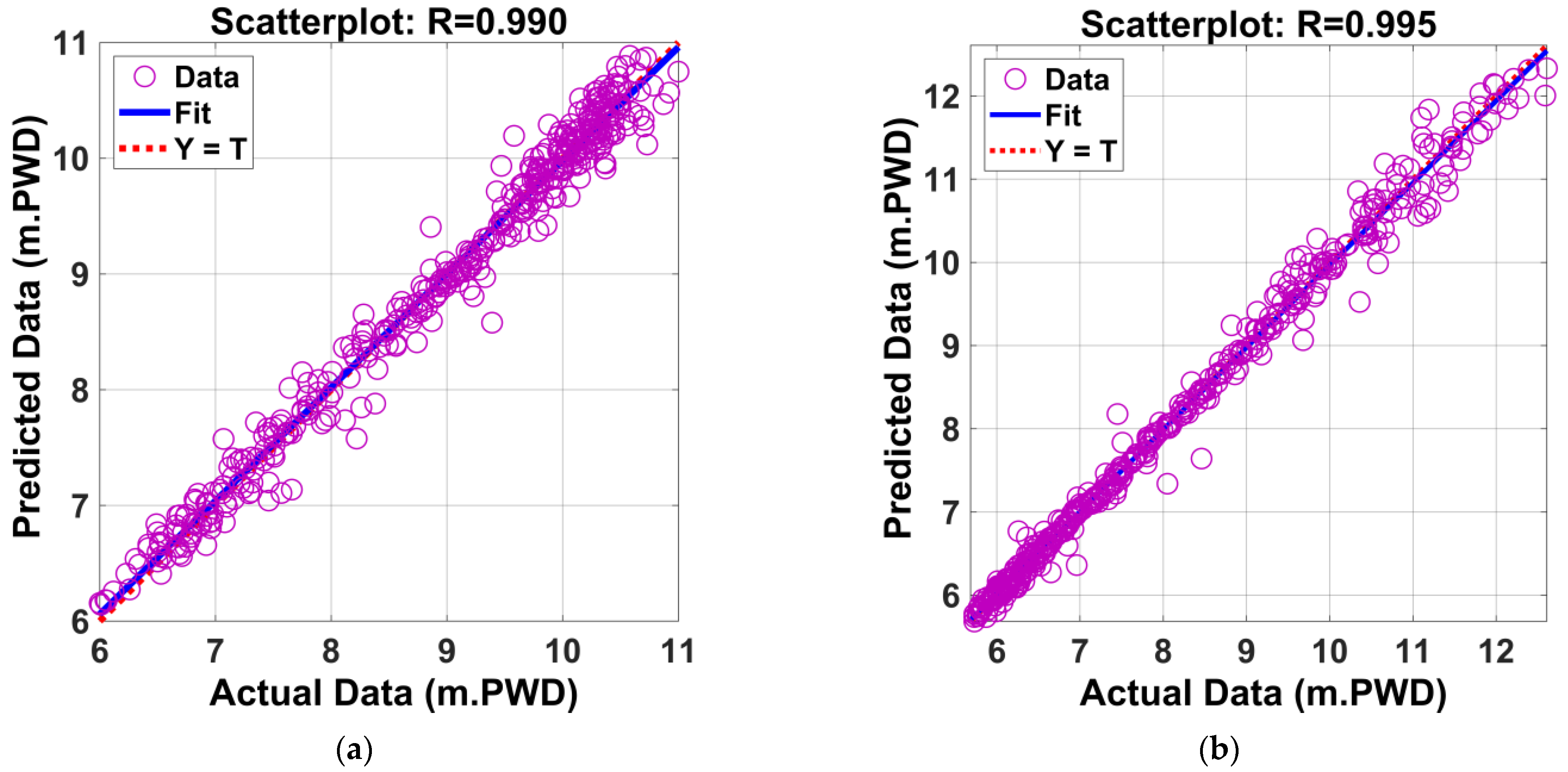
4.9.3. Model Accuracy via Regression Plot
5. Conclusions
- The ANN model (6-8-1) outperformed the ARIMA-based best model (SSE 15.143) by 53.043% and achieved the highest predictive accuracy with an SSE 9.894.
- The multivariate ANN model showed 9.241% higher accuracy than the best univariate ANN model.
- The ARIMAX model improved prediction accuracy by 9.522% over the best ARIMA model.
- It is evident that models that included exogenous variables provided more reliable GWL predictions than univariate models.
Author Contributions
Funding
Data Availability Statement
Acknowledgments
Conflicts of Interest
Appendix A. Data Details

| Week | RFt (mm) | Week | RFt (mm) | Week | RFt (mm) | Week | RFt (mm) |
|---|---|---|---|---|---|---|---|
| 3 March 2003 | 0.00 | 16 February 2004 | 0.00 | 31 January 2005 | 0.00 | 16 January 2006 | 0.00 |
| 10 March 2003 | 0.00 | 23 February 2004 | 0.00 | 7 February 2005 | 0.00 | 23 January 2006 | 0.00 |
| 17 March 2003 | 33.00 | 1 March 2004 | 0.00 | 14 February 2005 | 0.00 | 30 January 2006 | 0.00 |
| 24 March 2003 | 32.50 | 8 March 2004 | 0.00 | 21 February 2005 | 0.00 | 6 February 2006 | 0.00 |
| 31 March 2003 | 77.00 | 15 March 2004 | 0.00 | 28 February 2005 | 0.00 | 13 February 2006 | 0.00 |
| 7 April 2003 | 0.00 | 22 March 2004 | 0.00 | 7 March 2005 | 0.00 | 20 February 2006 | 0.00 |
| 14 April 2003 | 0.00 | 29 March 2004 | 0.00 | 14 March 2005 | 14.00 | 27 February 2006 | 0.00 |
| 21 April 2003 | 25.50 | 5 April 2004 | 0.00 | 21 March 2005 | 0.00 | 6 March 2006 | 0.00 |
| 28 April 2003 | 14.50 | 12 April 2004 | 6.70 | 28 March 2005 | 21.00 | 13 March 2006 | 0.00 |
| 5 May 2003 | 3.50 | 19 April 2004 | 0.00 | 4 April 2005 | 45.00 | 20 March 2006 | 0.00 |
| 12 May 2003 | 69.70 | 26 April 2004 | 24.00 | 11 April 2005 | 0.00 | 27 March 2006 | 0.00 |
| 19 May 2003 | 0.00 | 3 May 2004 | 26.00 | 18 April 2005 | 0.00 | 3 April 2006 | 10.00 |
| 26 May 2003 | 15.00 | 10 May 2004 | 0.00 | 25 April 2005 | 0.00 | 10 April 2006 | 14.00 |
| 2 June 2003 | 9.00 | 17 May 2004 | 0.00 | 2 May 2005 | 66.50 | 17 April 2006 | 0.00 |
| 9 June 2003 | 35.00 | 24 May 2004 | 82.00 | 9 May 2005 | 90.00 | 24 April 2006 | 18.00 |
| 16 June 2003 | 46.00 | 31 May 2004 | 59.50 | 16 May 2005 | 35.00 | 1 May 2006 | 0.00 |
| 23 June 2003 | 64.00 | 7 June 2004 | 60.00 | 23 May 2005 | 14.00 | 8 May 2006 | 61.40 |
| 30 June 2003 | 121.50 | 14 June 2004 | 32.00 | 30 May 2005 | 0.00 | 15 May 2006 | 11.00 |
| 7 July 2003 | 0.00 | 21 June 2004 | 116.30 | 6 June 2005 | 0.00 | 22 May 2006 | 0.00 |
| 14 July 2003 | 164.00 | 28 June 2004 | 62.50 | 13 June 2005 | 0.00 | 29 May 2006 | 146.00 |
| 21 July 2003 | 2.20 | 5 July 2004 | 26.00 | 20 June 2005 | 6.00 | 5 June 2006 | 77.00 |
| 28 July 2003 | 29.00 | 12 July 2004 | 28.00 | 27 June 2005 | 29.00 | 12 June 2006 | 51.00 |
| 4 August 2003 | 111.50 | 19 July 2004 | 70.00 | 4 July 2005 | 44.50 | 19 June 2006 | 50.00 |
| 11 August 2003 | 13.20 | 26 July 2004 | 161.80 | 11 July 2005 | 45.00 | 26 June 2006 | 39.00 |
| 18 August 2003 | 84.00 | 2 August 2004 | 44.50 | 18 July 2005 | 247.50 | 3 July 2006 | 12.00 |
| 25 August 2003 | 58.00 | 9 August 2004 | 19.00 | 25 July 2005 | 73.00 | 10 July 2006 | 99.00 |
| 1 September 2003 | 39.50 | 16 August 2004 | 47.00 | 1 August 2005 | 14.00 | 17 July 2006 | 29.00 |
| 8 September 2003 | 84.00 | 23 August 2004 | 12.00 | 8 August 2005 | 18.00 | 24 July 2006 | 46.00 |
| 15 September 2003 | 33.50 | 30 August 2004 | 28.50 | 15 August 2005 | 47.00 | 31 July 2006 | 63.50 |
| 22 September 2003 | 0.00 | 6 September 2004 | 75.00 | 22 August 2005 | 0.00 | 7 August 2006 | 7.50 |
| 29 September 2003 | 41.00 | 13 September 2004 | 188.00 | 29 August 2005 | 20.50 | 14 August 2006 | 62.00 |
| 6 October 2003 | 68.50 | 20 September 2004 | 340.00 | 5 September 2005 | 95.00 | 21 August 2006 | 23.00 |
| 13 October 2003 | 102.00 | 27 September 2004 | 20.00 | 12 September 2005 | 93.00 | 28 August 2006 | 34.00 |
| 20 October 2003 | 8.00 | 4 October 2004 | 95.00 | 19 September 2005 | 435.00 | 4 September 2006 | 59.00 |
| 27 October 2003 | 11.00 | 11 October 2004 | 117.50 | 26 September 2005 | 20.00 | 11 September 2006 | 27.00 |
| 3 November 2003 | 7.00 | 18 October 2004 | 24.00 | 3 October 2005 | 333.50 | 18 September 2006 | 95.00 |
| 10 November 2003 | 0.00 | 25 October 2004 | 0.00 | 10 October 2005 | 118.00 | 25 September 2006 | 339.00 |
| 17 November 2003 | 0.00 | 1 November 2004 | 0.00 | 17 October 2005 | 0.00 | 2 October 2006 | 22.00 |
| 24 November 2003 | 0.00 | 8 November 2004 | 0.00 | 24 October 2005 | 349.50 | 9 October 2006 | 0.00 |
| 1 December 2003 | 0.00 | 15 November 2004 | 0.00 | 31 October 2005 | 0.00 | 16 October 2006 | 0.00 |
| 8 December 2003 | 0.00 | 22 November 2004 | 0.00 | 7 November 2005 | 0.00 | 23 October 2006 | 0.00 |
| 15 December 2003 | 0.00 | 29 November 2004 | 0.00 | 14 November 2005 | 0.00 | 30 October 2006 | 0.00 |
| 22 December 2003 | 0.00 | 6 December 2004 | 0.00 | 21 November 2005 | 0.00 | 6 November 2006 | 0.00 |
| 29 December 2003 | 5.50 | 13 December 2004 | 0.00 | 28 November 2005 | 0.00 | 13 November 2006 | 10.00 |
| 5 January 2004 | 0.00 | 20 December 2004 | 0.00 | 5 December 2005 | 0.00 | 20 November 2006 | 0.00 |
| 12 January 2004 | 0.00 | 27 December 2004 | 0.00 | 12 December 2005 | 0.00 | 27 November 2006 | 0.00 |
| 19 January 2004 | 0.00 | 3 January 2005 | 0.00 | 19 December 2005 | 0.00 | 4 December 2006 | 0.00 |
| 26 January 2004 | 2.00 | 10 January 2005 | 0.00 | 26 December 2005 | 0.00 | 11 December 2006 | 0.00 |
| 2 February 2004 | 0.00 | 17 January 2005 | 0.00 | 2 January 2006 | 0.00 | 18 December 2006 | 0.00 |
| 9 February 2004 | 0.00 | 24 January 2005 | 19.00 | 9 January 2006 | 0.00 | 25 December 2006 | 0.00 |
| Week | GWLt (m.PWD) | Week | GWLt (m.PWD) | Week | GWLt (m.PWD) | Week | GWLt (m.PWD) |
|---|---|---|---|---|---|---|---|
| 3 March 2003 | 6.65 | 16 February 2004 | 7.36 | 31 January 2005 | 7.25 | 16 January 2006 | 7.65 |
| 10 March 2003 | 6.56 | 23 February 2004 | 7.24 | 7 February 2005 | 7.12 | 23 January 2006 | 7.42 |
| 17 March 2003 | 6.49 | 1 March 2004 | 7.10 | 14 February 2005 | 6.99 | 30 January 2006 | 7.27 |
| 24 March 2003 | 6.43 | 8 March 2004 | 6.96 | 21 February 2005 | 6.88 | 6 February 2006 | 7.11 |
| 31 March 2003 | 6.36 | 15 March 2004 | 6.82 | 28 February 2005 | 6.78 | 13 February 2006 | 6.95 |
| 7 April 2003 | 6.29 | 22 March 2004 | 6.68 | 7 March 2005 | 6.63 | 20 February 2006 | 6.84 |
| 14 April 2003 | 6.21 | 29 March 2004 | 6.56 | 14 March 2005 | 6.57 | 27 February 2006 | 6.71 |
| 21 April 2003 | 6.14 | 5 April 2004 | 6.44 | 21 March 2005 | 6.45 | 6 March 2006 | 6.58 |
| 28 April 2003 | 6.20 | 12 April 2004 | 6.96 | 28 March 2005 | 6.37 | 13 March 2006 | 6.46 |
| 5 May 2003 | 6.01 | 19 April 2004 | 6.26 | 4 April 2005 | 6.30 | 20 March 2006 | 6.35 |
| 12 May 2003 | 6.09 | 26 April 2004 | 6.22 | 11 April 2005 | 6.22 | 27 March 2006 | 6.24 |
| 19 May 2003 | 6.05 | 3 May 2004 | 6.18 | 18 April 2005 | 6.12 | 3 April 2006 | 6.12 |
| 26 May 2003 | 6.02 | 10 May 2004 | 6.12 | 25 April 2005 | 6.01 | 10 April 2006 | 6.06 |
| 2 June 2003 | 6.00 | 17 May 2004 | 6.06 | 2 May 2005 | 5.98 | 17 April 2006 | 5.95 |
| 9 June 2003 | 6.02 | 24 May 2004 | 6.15 | 9 May 2005 | 5.98 | 24 April 2006 | 5.86 |
| 16 June 2003 | 6.06 | 31 May 2004 | 6.27 | 16 May 2005 | 5.96 | 1 May 2006 | 5.81 |
| 23 June 2003 | 6.24 | 7 June 2004 | 6.32 | 23 May 2005 | 5.93 | 8 May 2006 | 5.77 |
| 30 June 2003 | 6.53 | 14 June 2004 | 6.36 | 30 May 2005 | 5.89 | 15 May 2006 | 5.73 |
| 7 July 2003 | 6.90 | 21 June 2004 | 6.42 | 6 June 2005 | 5.83 | 22 May 2006 | 5.73 |
| 14 July 2003 | 7.43 | 28 June 2004 | 6.63 | 13 June 2005 | 5.83 | 29 May 2006 | 5.73 |
| 21 July 2003 | 8.05 | 5 July 2004 | 6.92 | 20 June 2005 | 5.79 | 5 June 2006 | 5.78 |
| 28 July 2003 | 8.56 | 12 July 2004 | 7.22 | 27 June 2005 | 5.89 | 12 June 2006 | 5.99 |
| 4 August 2003 | 9.01 | 19 July 2004 | 7.80 | 4 July 2005 | 6.07 | 19 June 2006 | 6.23 |
| 11 August 2003 | 9.34 | 26 July 2004 | 8.55 | 11 July 2005 | 6.33 | 26 June 2006 | 6.39 |
| 18 August 2003 | 9.70 | 2 August 2004 | 9.07 | 18 July 2005 | 6.85 | 3 July 2006 | 6.57 |
| 25 August 2003 | 10.07 | 9 August 2004 | 9.37 | 25 July 2005 | 7.44 | 10 July 2006 | 6.74 |
| 1 September 2003 | 10.44 | 16 August 2004 | 9.56 | 1 August 2005 | 7.45 | 17 July 2006 | 7.10 |
| 8 September 2003 | 10.66 | 23 August 2004 | 9.76 | 8 August 2005 | 8.30 | 24 July 2006 | 7.49 |
| 15 September 2003 | 11.13 | 30 August 2004 | 10.06 | 15 August 2005 | 8.90 | 31 July 2006 | 7.95 |
| 22 September 2003 | 11.26 | 6 September 2004 | 10.40 | 22 August 2005 | 9.13 | 7 August 2006 | 8.34 |
| 29 September 2003 | 11.60 | 13 September 2004 | 10.55 | 29 August 2005 | 9.59 | 14 August 2006 | 8.68 |
| 6 October 2003 | 11.61 | 20 September 2004 | 10.66 | 5 September 2005 | 9.92 | 21 August 2006 | 8.82 |
| 13 October 2003 | 11.60 | 27 September 2004 | 11.14 | 12 September 2005 | 9.85 | 28 August 2006 | 9.11 |
| 20 October 2003 | 11.10 | 4 October 2004 | 11.13 | 19 September 2005 | 9.67 | 4 September 2006 | 9.50 |
| 27 October 2003 | 10.67 | 11 October 2004 | 11.57 | 26 September 2005 | 9.65 | 11 September 2006 | 9.75 |
| 3 November 2003 | 10.46 | 18 October 2004 | 11.19 | 3 October 2005 | 10.36 | 18 September 2006 | 9.92 |
| 10 November 2003 | 10.08 | 25 October 2004 | 10.66 | 10 October 2005 | 10.56 | 25 September 2006 | 10.57 |
| 17 November 2003 | 9.84 | 1 November 2004 | 10.19 | 17 October 2005 | 10.91 | 2 October 2006 | 10.65 |
| 24 November 2003 | 9.54 | 8 November 2004 | 9.87 | 24 October 2005 | 11.42 | 9 October 2006 | 10.34 |
| 1 December 2003 | 9.30 | 15 November 2004 | 9.60 | 31 October 2005 | 10.88 | 16 October 2006 | 9.96 |
| 8 December 2003 | 9.06 | 22 November 2004 | 9.29 | 7 November 2005 | 10.37 | 23 October 2006 | 9.56 |
| 15 December 2003 | 8.82 | 29 November 2004 | 9.01 | 14 November 2005 | 9.89 | 30 October 2006 | 9.22 |
| 22 December 2003 | 8.65 | 6 December 2004 | 8.74 | 21 November 2005 | 9.52 | 6 November 2006 | 8.93 |
| 29 December 2003 | 8.46 | 13 December 2004 | 8.50 | 28 November 2005 | 9.21 | 13 November 2006 | 8.67 |
| 5 January 2004 | 8.28 | 20 December 2004 | 8.24 | 5 December 2005 | 8.94 | 20 November 2006 | 8.43 |
| 12 January 2004 | 8.11 | 27 December 2004 | 8.04 | 12 December 2005 | 8.67 | 27 November 2006 | 8.26 |
| 19 January 2004 | 7.91 | 3 January 2005 | 7.85 | 19 December 2005 | 8.44 | 4 December 2006 | 8.05 |
| 26 January 2004 | 7.76 | 10 January 2005 | 7.66 | 26 December 2005 | 8.21 | 11 December 2006 | 7.85 |
| 2 February 2004 | 7.61 | 17 January 2005 | 7.48 | 2 January 2006 | 7.99 | 18 December 2006 | 7.67 |
| 9 February 2004 | 7.47 | 24 January 2005 | 7.37 | 9 January 2006 | 7.81 | 25 December 2006 | 7.51 |
References
- Hossain, M.B.; Roy, D.; Mahmud, M.N.H.; Paul, P.L.C.; Yesmin, M.S.; Kundu, P.K. Early transplanting of rainfed rice minimizes irrigation demand by utilizing rainfall. Environ. Syst. Res. 2021, 10, 34. [Google Scholar] [CrossRef]
- Adhikary, S.K.; Das, S.K.; Chaki, T.; Rahman, M. Identifying safe drinking water source for establishing sustainable urban water supply scheme in Rangunia municipality, Bangladesh. In Proceedings of the 20th International Congress on Modelling and Simulation, Adelaide, Australia, 1–6 December 2013; pp. 3134–3140. [Google Scholar]
- Lu, Y.; Dai, L.; Yan, G.; Huo, Z.; Chen, W.; Lan, J.; Zhang, C.; Xu, Q.; Deng, S.; Chen, J. Effects of various land utilization types on groundwater at different temporal scales: A case study of Huocheng plain, Xinjiang, China. Front. Environ. Sci. 2023, 11, 1225916. [Google Scholar] [CrossRef]
- Mishra, N.; Khare, D.; Gupta, K.K.; Shukla, R. Impact of land use change on groundwater—A review. Adv. Water Resour. Prot. 2014, 2, 28–41. [Google Scholar]
- Wada, Y.; Van Beek, L.P.; Van Kempen, C.M.; Reckman, J.W.; Vasak, S.; Bierkens, M.F. Global depletion of groundwater resources. Geophys. Res. Lett. 2010, 37, L20402. [Google Scholar] [CrossRef]
- Foster, S.; Pulido-Bosch, A.; Vallejos, Á.; Molina, L.; Llop, A.; MacDonald, A.M. Impact of irrigated agriculture on groundwater-recharge salinity: A major sustainability concern in semi-arid regions. Hydrogeol. J. 2018, 26, 2781–2791. [Google Scholar] [CrossRef]
- Schmoll, O. (Ed.) Protecting Groundwater for Health: Managing the Quality of Drinking-Water Sources; World Health Organization: Geneva, Switzerland, 2006. [Google Scholar]
- Shahid, S.; Wang, X.J.; Moshiur Rahman, M.; Hasan, R.; Harun, S.B.; Shamsudin, S. Spatial assessment of groundwater over-exploitation in northwestern districts of Bangladesh. J. Geol. Soc. India 2015, 85, 463–470. [Google Scholar] [CrossRef]
- Dangar, S.; Asoka, A.; Mishra, V. Causes and implications of groundwater depletion in India: A review. J. Hydrol. 2021, 596, 126103. [Google Scholar] [CrossRef]
- Jain, M.; Fishman, R.; Mondal, P.; Galford, G.L.; Bhattarai, N.; Naeem, S.; Lall, U.; Balwinder-Singh; DeFries, R.S. Groundwater depletion will reduce cropping intensity in India. Sci. Adv. 2021, 7, eabd2849. [Google Scholar] [CrossRef]
- Jia, X.; O’Connor, D.; Hou, D.; Jin, Y.; Li, G.; Zheng, C.; Ok, Y.S.; Tsang, D.C.; Luo, J. Groundwater depletion and contamination: Spatial distribution of groundwater resources sustainability in China. Sci. Total Environ. 2019, 672, 551–562. [Google Scholar] [CrossRef] [PubMed]
- Islam, F.; Imteaz, M.A. The effectiveness of ARIMAX model for prediction of summer rainfall in northwest Western Australia. IOP Conf. Ser. Mater. Sci. Eng. 2021, 1067, 012037. [Google Scholar] [CrossRef]
- Hossain, M.Z.; Adhikary, S.K. Identifying groundwater recharge potential zones in Barind Tract of Bangladesh using geospatial technique. AIP Conf. Proc. 2023, 2713, 050001. [Google Scholar] [CrossRef]
- Hossain, M.Z.; Adhikary, S.K.; Nath, H.; Kafy, A.A.; Altuwaijri, H.A.; Rahman, M.T. Integrated Geospatial and Analytical Hierarchy Process Approach for Assessing Sustainable Management of Groundwater Recharge Potential in Barind Tract. Water 2024, 16, 2918. [Google Scholar] [CrossRef]
- Mancini, S.; Egidio, E.; De Luca, D.A.; Lasagna, M. Application and comparison of different statistical methods for the analysis of groundwater levels over time: Response to rainfall and resource evolution in the Piedmont Plain (NW Italy). Sci. Total Environ. 2022, 846, 157479. [Google Scholar] [CrossRef]
- Sekhar, P.H.; Kesavulu Poola, K.; Bhupathi, M. Modelling and prediction of coastal Andhra rainfall using ARIMA and ANN models. Int. J. Stat. Appl. Math. 2020, 5, 104–110. [Google Scholar]
- Elbeltagi, A.; Salam, R.; Pal, S.C.; Zerouali, B.; Shahid, S.; Mallick, J.; Islam, M.S.; Islam, A.R.M.T. Groundwater level estimation in northern region of Bangladesh using hybrid locally weighted linear regression and Gaussian process regression modeling. Theor. Appl. Climatol. 2022, 149, 131–151. [Google Scholar] [CrossRef]
- Sun, J.; Hu, L.; Li, D.; Sun, K.; Yang, Z. Data-driven models for accurate groundwater level prediction and their practical significance in groundwater management. J. Hydrol. Reg. Stud. 2022, 608, 127630. [Google Scholar] [CrossRef]
- Iqbal, N.; Khan, A.N.; Rizwan, A.; Ahmad, R.; Kim, B.W.; Kim, K.; Kim, D.H. Groundwater level prediction model using correlation and difference mechanisms based on boreholes data for sustainable hydraulic resource management. IEEE Access 2021, 9, 96092–96113. [Google Scholar] [CrossRef]
- Qadir, B.H.; Mohammed, M.A. Comparison between SARIMA and SARIMAX time series Models with application on Groundwater in Sulaymaniyah. Sci. J. Cihan Univ. Sulaimaniya 2021, 5, 30–48. [Google Scholar]
- Shahinuzzaman, M.; Haque, M.N.; Uddin, K.M.N.; Alibuddin, M. Identification of Aquifer Properties in the Eastern Part of Kushtia District, Bangladesh. J. Geosci. Environ. Prot. 2020, 8, 222. [Google Scholar] [CrossRef]
- Porte, P.; Isaac, R.K.; Mahilang, K.K.S.; Sonboier, K.; Minj, P. Groundwater level prediction using artificial neural network model. Int. J. Curr. Microbiol. Appl. Sci. 2018, 72, 2947–2954. [Google Scholar] [CrossRef]
- Ghazi, B.; Jeihouni, E.; Kalantari, Z. Predicting groundwater level fluctuations under climate change scenarios for Tasuj plain, Iran. Arab. J. Geosci. 2021, 14, 115. [Google Scholar] [CrossRef]
- Kassem, A.A.; Raheem, A.M.; Khidir, K.M. Daily streamflow prediction for khazir river basin using ARIMA and ANN models. ZANCO J. Pure Appl. Sci. 2020, 32, 30–39. [Google Scholar]
- Narvekar, M.; Fargose, P. Daily weather forecasting using artificial neural network. Int. J. Comput. Appl. 2015, 121, 0975–8887. [Google Scholar] [CrossRef]
- Liu, Q.; Zou, Y.; Liu, X.; Linge, N. A survey on rainfall forecasting using artificial neural network. Int. J. Embed. Syst. 2019, 11, 240–249. [Google Scholar] [CrossRef]
- Khedri, A.; Kalantari, N.; Vadiati, M. Comparison study of artificial intelligence method for short term groundwater level prediction in the northeast Gachsaran unconfined aquifer. Water Supply 2020, 20, 909–921. [Google Scholar] [CrossRef]
- Husna, N.E.A.; Bari, S.H.; Hussain, M.M.; Ur-rahman, M.T.; Rahman, M. Ground water level prediction using artificial neural network. Int. J. Hydrol. Sci. Technol. 2016, 6, 371–381. [Google Scholar] [CrossRef]
- Pham, Q.B.; Kumar, M.; Di Nunno, F.; Elbeltagi, A.; Granata, F.; Islam, A.R.M.T.; Talukdar, S.; Nguyen, X.C.; Ahmed, A.N.; Anh, D.T. Groundwater level prediction using machine learning algorithms in a drought-prone area. Neural Comput. Appl. 2022, 34, 10751–10773. [Google Scholar] [CrossRef]
- Palani, S.; Liong, S.Y.; Tkalich, P. An ANN application for water quality forecasting. Mar. Pollut. 2008, 56, 1586–1597. [Google Scholar] [CrossRef] [PubMed]
- Rabbi, F.; Tareq, S.U.; Islam, M.M.; Chowdhury, M.A.; Kashem, M.A. A multivariate time series approach for forecasting of electricity demand in bangladesh using arimax model. In Proceedings of the 2020 2nd International Conference on Sustainable Technologies for Industry 4.0, Dhaka, Bangladesh, 19–20 December 2020; pp. 1–5. [Google Scholar]
- Lemos, J.D.J.S.; Bezerra, F.N.R. ARIMAX Model to Forecast Grain Production under Rainfall Instabilities in Brazilian Semi-Arid Region. Glob. J. Hum. Soc. Sci. 2024, 24, 1–9. [Google Scholar]
- Khairi, S.M.; Aziz, I.A. Domestic water consumption forecasting with sociodemographic features using ARIMA and ARIMAX: A case study in Malaysia. Platf. A J. Sci. Technol. 2022, 5, 16–30. [Google Scholar] [CrossRef]
- Jalalkamali, A.; Moradi, M.; Moradi, N. Application of several artificial intelligence models and ARIMAX model for forecasting drought using the Standardized Precipitation Index. Int. J. Environ. Sci. Technol. 2015, 12, 1201–1210. [Google Scholar] [CrossRef]
- Khandelwal, I.; Adhikari, R.; Verma, G. Time series forecasting using hybrid ARIMA and ANN models based on DWT decomposition. Procedia Comput. Sci. 2015, 48, 173–179. [Google Scholar] [CrossRef]
- Chitsazan, M.; Rahmani, G.; Neyamadpour, A. Forecasting groundwater level by artificial neural networks as an alternative approach to groundwater modeling. J. Geol. Soc. India 2015, 85, 98–106. [Google Scholar] [CrossRef]
- Wang, W.; Van Gelder, P.H.; Vrijling, J.K.; Ma, J. Forecasting daily streamflow using hybrid ANN models. J. Hydrol. Reg. Stud. 2006, 324, 383–399. [Google Scholar] [CrossRef]
- Azad, A.S.; Sokkalingam, R.; Daud, H.; Adhikary, S.K.; Khurshid, H.; Mazlan, S.N.A.; Rabbani, M.B.A. Water level prediction through hybrid SARIMA and ANN models based on time series analysis: Red hills reservoir case study. Sustainability 2022, 14, 1843. [Google Scholar] [CrossRef]
- Islam, F.; Imteaz, M.A. Use of teleconnections to predict Western Australian seasonal rainfall using ARIMAX model. Hydrology 2020, 7, 52. [Google Scholar] [CrossRef]
- Pourmorad, S.; Kabolizade, M.; Dimuccio, L.A. Artificial Intelligence Advancements for Accurate Groundwater Level Modelling: An Updated Synthesis and Review. Appl. Sci. 2024, 14, 7358. [Google Scholar] [CrossRef]
- Li, W.; Finsa, M.M.; Laskey, K.B.; Houser, P.; Douglas-Bate, R. Groundwater level prediction with machine learning to support sustainable irrigation in water scarcity regions. Water 2023, 15, 3473. [Google Scholar] [CrossRef]
- Haji-Aghajany, S.; Amerian, Y.; Amiri-Simkooei, A. Impact of climate change parameters on groundwater level: Implications for two subsidence regions in Iran using geodetic observations and artificial neural networks (ANN). Remote Sens. 2023, 15, 1555. [Google Scholar] [CrossRef]
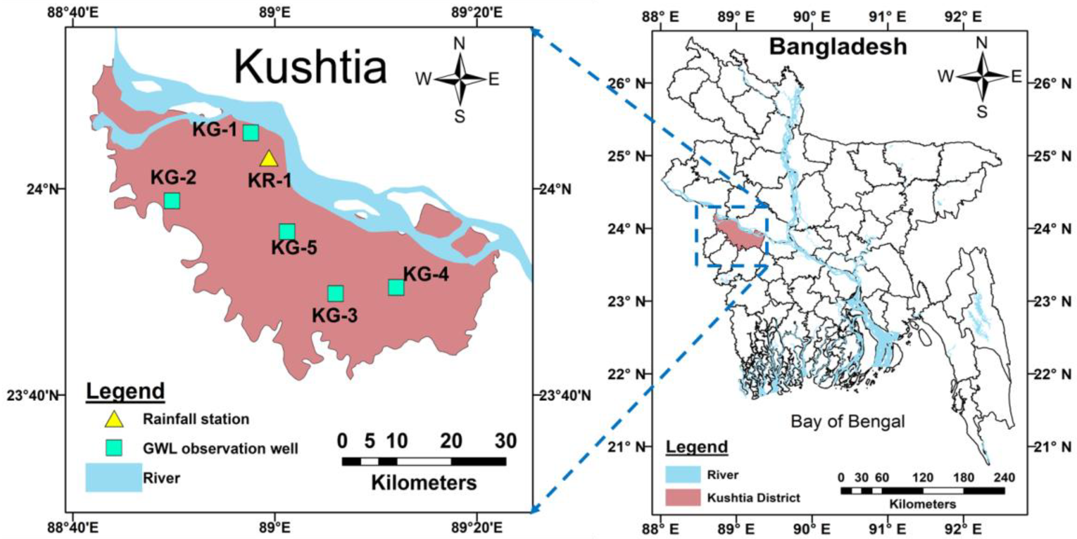
| SL No | Station ID | Station Type | Location of Station (Sub-District Name) | Latitude (Degree) | Longitude (Degree) |
|---|---|---|---|---|---|
| 1 | KG-1 | GWL | Bheramara | 24.09 | 88.96 |
| 2 | KG-2 | GWL | Daulatpur | 23.98 | 88.83 |
| 3 | KG-3 | GWL | Kushtia Sadar | 23.83 | 89.10 |
| 4 | KG-4 | GWL | Kumarkhali | 23.84 | 89.20 |
| 5 | KG-5 | GWL | Mirpur | 23.93 | 89.02 |
| 6 | KR-1 | RF | Mirpur | 24.05 | 88.99 |
| Station ID | Location | Model Architecture | Model Performance | ||
|---|---|---|---|---|---|
| RMSE | NSE | SSE | |||
| KG-1 | Bheramara | ANN 6-8-1 | 0.154 | 0.988 | 9.894 |
| KG-2 | Daulatpur | ANN 7-8-1 | 0.168 | 0.979 | 11.799 |
| KG-3 | Kushtia Sadar | ANN 10-4-1 | 0.231 | 0.965 | 26.910 |
| KG-4 | Kumarkhali | ANN 6-7-1 | 0.255 | 0.986 | 22.273 |
| KG-5 | Mirpur | ANN 8-9-1 | 0.180 | 0.984 | 13.434 |
| Station ID | Location | Model Architecture | Model Performance | ||
|---|---|---|---|---|---|
| RMSE | NSE | SSE | |||
| KG-1 | Bheramara | ANN 3-7-1 | 0.161 | 0.987 | 10.809 |
| KG-2 | Daulatpur | ANN 2-3-1 | 0.171 | 0.979 | 12.171 |
| KG-3 | Kushtia Sadar | ANN 4-9-1 | 0.258 | 0.957 | 26.802 |
| KG-4 | Kumarkhali | ANN 2-4-1 | 0.254 | 0.986 | 27.725 |
| KG-5 | Mirpur | ANN 5-10-1 | 0.181 | 0.984 | 13.595 |
| Model | Training | Validation | Test | |||
|---|---|---|---|---|---|---|
| MSE | NSE | MSE | NSE | MSE | NSE | |
| ANN 8-2-1 | 0.030 | 0.984 | 0.066 | 0.964 | 0.046 | 0.978 |
| ANN 8-3-1 | 0.032 | 0.982 | 0.061 | 0.967 | 0.045 | 0.978 |
| ANN 8-4-1 | 0.046 | 0.975 | 0.069 | 0.963 | 0.076 | 0.963 |
| ANN 8-5-1 | 0.036 | 0.980 | 0.074 | 0.960 | 0.037 | 0.982 |
| ANN 8-6-1 | 0.031 | 0.983 | 0.078 | 0.958 | 0.042 | 0.980 |
| ANN 8-7-1 | 0.030 | 0.983 | 0.201 | 0.892 | 0.040 | 0.981 |
| ANN 8-8-1 | 0.035 | 0.981 | 0.079 | 0.958 | 0.042 | 0.980 |
| ANN 8-9-1 | 0.032 | 0.983 | 0.083 | 0.955 | 0.032 | 0.984 |
| ANN 8-10-1 | 0.027 | 0.985 | 0.071 | 0.962 | 0.039 | 0.981 |
| Station ID | Location | Model Architecture | Model Performance (SSE) |
|---|---|---|---|
| KG-1 | Bheramara | ARIMAX (3,0,3) | 15.361 |
| KG-2 | Daulatpur | ARIMAX (3,0,2) | 18.721 |
| KG-3 | Kushtia Sadar | ARIMAX (1,0,3) | 25.449 |
| KG-4 | Kumarkhali | ARIMAX (2,0,0) | 63.680 |
| KG-5 | Mirpur | ARIMAX (3,0,2) | 15.143 |
| Station ID | Location | Model Architecture | Model Performance (SSE) |
|---|---|---|---|
| KG-1 | Bheramara | ARIMA (2,0,1) | 17.217 |
| KG-2 | Daulatpur | ARIMA (2,0,1) | 26.880 |
| KG-3 | Kushtia Sadar | ARIMA (2,0,3) | 28.207 |
| KG-4 | Kumarkhali | ARIMA (3,0,1) | 64.582 |
| KG-5 | Mirpur | ARIMA (2,0,1) | 16.585 |
| Model | SSE | MSE | RMSE | AIC | BIC |
|---|---|---|---|---|---|
| ARIMA (0,2,1) | 20.688 | 0.050 | 0.224 | −59.599 | −47.521 |
| ARIMA (1,2,2) | 20.688 | 0.050 | 0.224 | −55.600 | −35.471 |
| ARIMA (1,2,3) | 20.680 | 0.050 | 0.223 | −53.750 | −29.594 |
| ARIMA (2,0,0) | 21.220 | 0.051 | 0.226 | −47.077 | −30.974 |
| ARIMA (2,0,1) | 16.585 | 0.040 | 0.200 | −147.100 | −126.971 |
| ARIMA (2,0,2) | 16.519 | 0.040 | 0.200 | −146.764 | −122.609 |
| ARIMA (3,0,1) | 16.537 | 0.040 | 0.200 | −146.317 | −122.162 |
| ARIMA (3,2,1) | 20.627 | 0.050 | 0.223 | −54.820 | −30.665 |
| ARIMA (3,2,2) | 20.563 | 0.050 | 0.223 | −54.092 | −25.911 |
| ARIMA (3,2,3) | 20.021 | 0.048 | 0.220 | −63.151 | −30.944 |
| Parameters | Value | Standard Error | T Statistic | p Value |
|---|---|---|---|---|
| Constant | 0.131 | 0.009 | 14.352 | 1.02 × 10−46 |
| AR{1} | 1.969 | 0.008 | 244.540 | 0 |
| AR{2} | −0.984 | 0.007 | −123.057 | 0 |
| MA{1} | −0.931 | 0.020 | −45.921 | 0 |
| Variance | 0.040 | 0.002 | 19.147 | 1.02 × 10−81 |
| Station ID | Location | Model/Data | Highest (m.PWD) | Lowest (m.PWD) | Average (m.PWD) |
|---|---|---|---|---|---|
| KG-1 | Bheramara | Existing (actual data) | 12.610 | 5.730 | 8.148 |
| KG-1 | Bheramara | ANN 6-8-1 (multivariate) | 10.797 | 5.875 | 7.742 |
| KG-5 | Mirpur | ARIMAX (3,0,2) | 11.694 | 6.622 | 8.951 |
| Performance Comparison of the Models | Remarks | ||||||
|---|---|---|---|---|---|---|---|
| Station ID | Results (SSE) | Model Architecture | ANN (Multivariate) (%) | ANN (Univariate) (%) | ARIMAX (%) | ARIMA (%) | |
| KG-1 | 9.894 | ANN 6-8-1 (multivariate) | 0 | −8.459 | −34.658 | −40.340 | Reference model ANN (multivariate): Performance Enhancement: -; Performance Degradation: ANN (univariate), ARIMAX, ARIMA |
| KG-1 | 10.809 | ANN 3-7-1 (univariate) | 9.241 | 0 | −28.620 | −34.826 | Reference model ANN (univariate): Performance Enhancement: ANN (multivariate); Performance Degradation: ARIMAX, ARIMA |
| KG-5 | 15.143 | ARIMAX (3,0,2) | 53.043 | 40.096 | 0 | −8.694 | Reference model ARIMAX: Performance Enhancement: ANN (multivariate), ANN (univariate); Performance Degradation: ARIMA |
| KG-1 | 16.585 | ARIMA (2,0,1) | 67.616 | 53.436 | 9.522 | 0 | Reference model ARIMA: Performance Enhancement: ANN (multivariate), ANN (univariate), ARIMAX; Performance Degradation: - |
Disclaimer/Publisher’s Note: The statements, opinions and data contained in all publications are solely those of the individual author(s) and contributor(s) and not of MDPI and/or the editor(s). MDPI and/or the editor(s) disclaim responsibility for any injury to people or property resulting from any ideas, methods, instructions or products referred to in the content. |
© 2024 by the authors. Licensee MDPI, Basel, Switzerland. This article is an open access article distributed under the terms and conditions of the Creative Commons Attribution (CC BY) license (https://creativecommons.org/licenses/by/4.0/).
Share and Cite
Hoque, M.A.; Apon, A.A.; Hassan, M.A.; Adhikary, S.K.; Islam, M.A. Enhanced Forecasting of Groundwater Level Incorporating an Exogenous Variable: Evaluating Conventional Multivariate Time Series and Artificial Neural Network Models. Geographies 2025, 5, 1. https://doi.org/10.3390/geographies5010001
Hoque MA, Apon AA, Hassan MA, Adhikary SK, Islam MA. Enhanced Forecasting of Groundwater Level Incorporating an Exogenous Variable: Evaluating Conventional Multivariate Time Series and Artificial Neural Network Models. Geographies. 2025; 5(1):1. https://doi.org/10.3390/geographies5010001
Chicago/Turabian StyleHoque, Md Abrarul, Asib Ahmmed Apon, Md Arafat Hassan, Sajal Kumar Adhikary, and Md Ariful Islam. 2025. "Enhanced Forecasting of Groundwater Level Incorporating an Exogenous Variable: Evaluating Conventional Multivariate Time Series and Artificial Neural Network Models" Geographies 5, no. 1: 1. https://doi.org/10.3390/geographies5010001
APA StyleHoque, M. A., Apon, A. A., Hassan, M. A., Adhikary, S. K., & Islam, M. A. (2025). Enhanced Forecasting of Groundwater Level Incorporating an Exogenous Variable: Evaluating Conventional Multivariate Time Series and Artificial Neural Network Models. Geographies, 5(1), 1. https://doi.org/10.3390/geographies5010001