
A Simplified Approach to Understanding Body Cooling Behavior and Estimating the Postmortem Interval


Abstract
:1. Introduction
2. Materials and Methods
3. Results
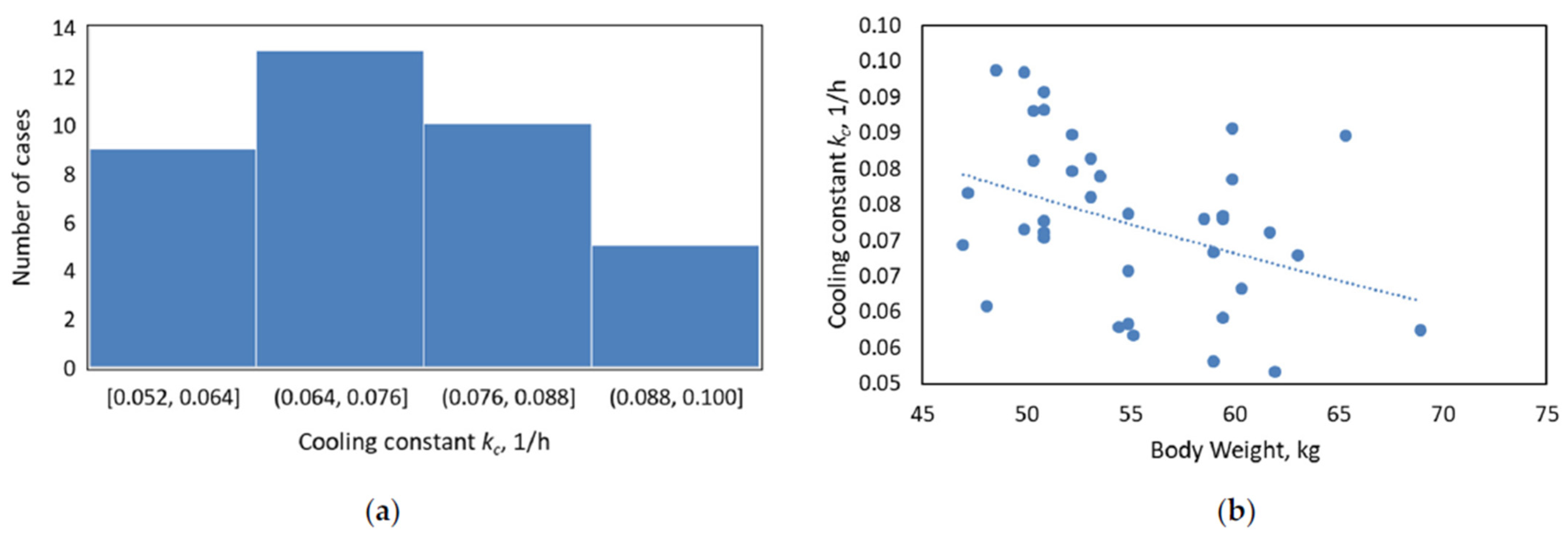
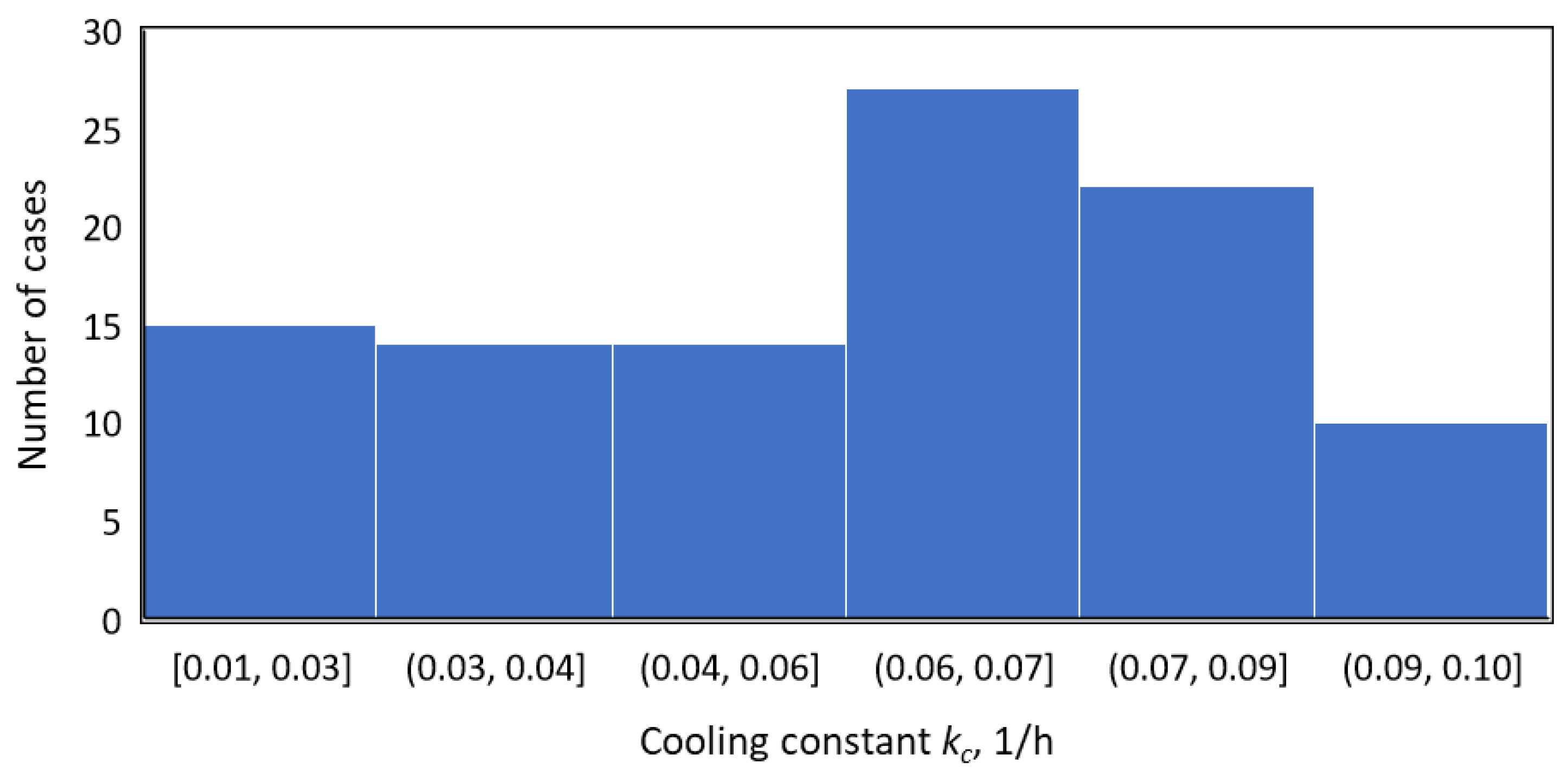
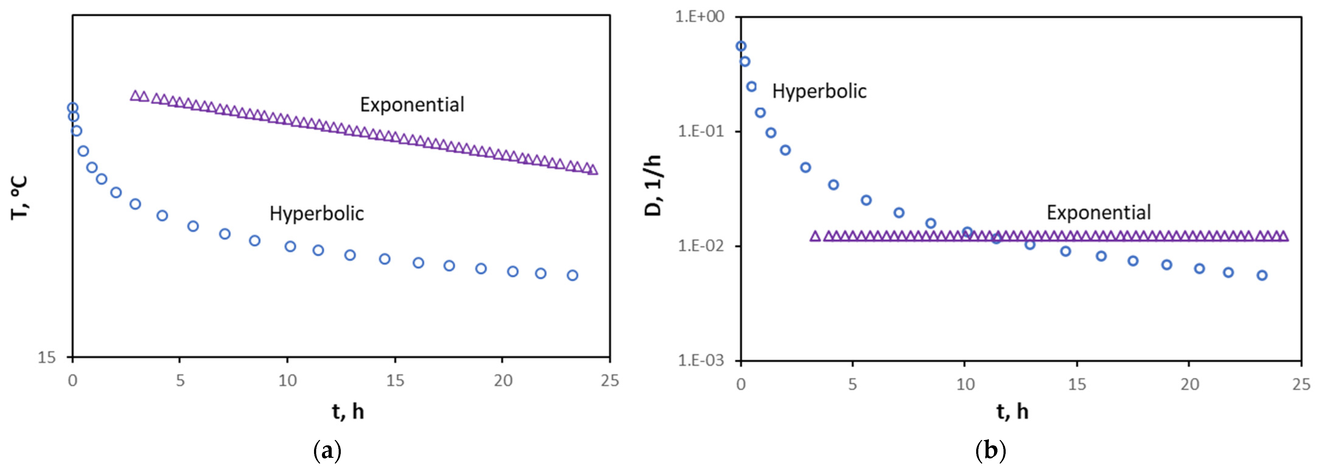
3.1. Understanding the Significance of Cooling Constant, kc
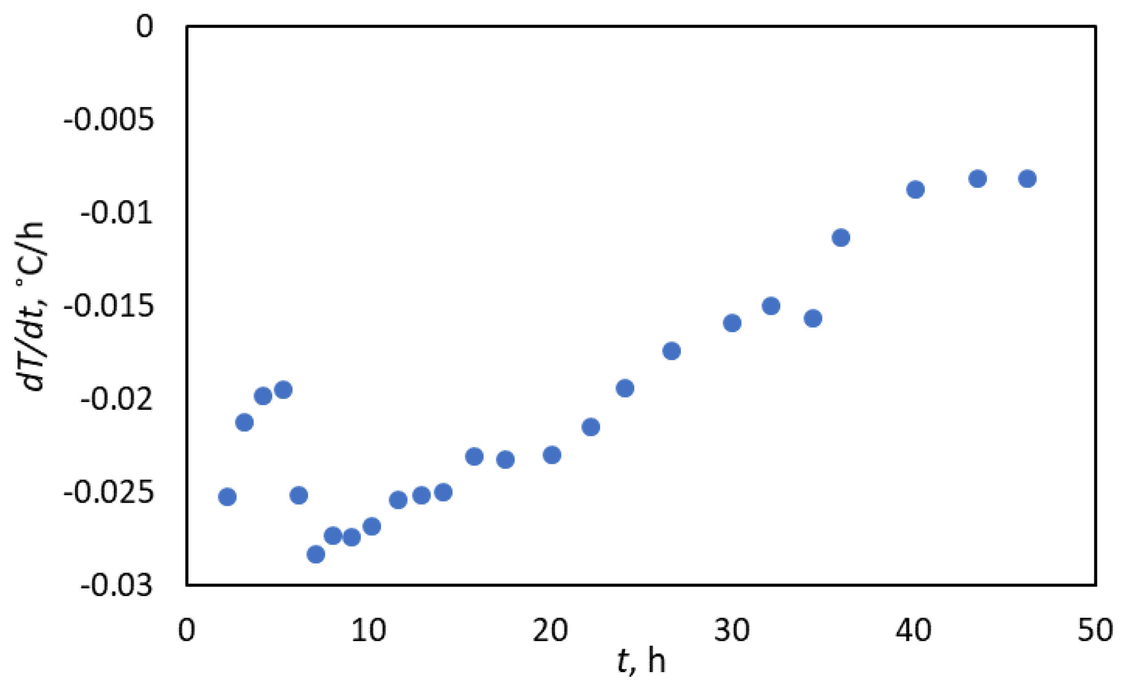
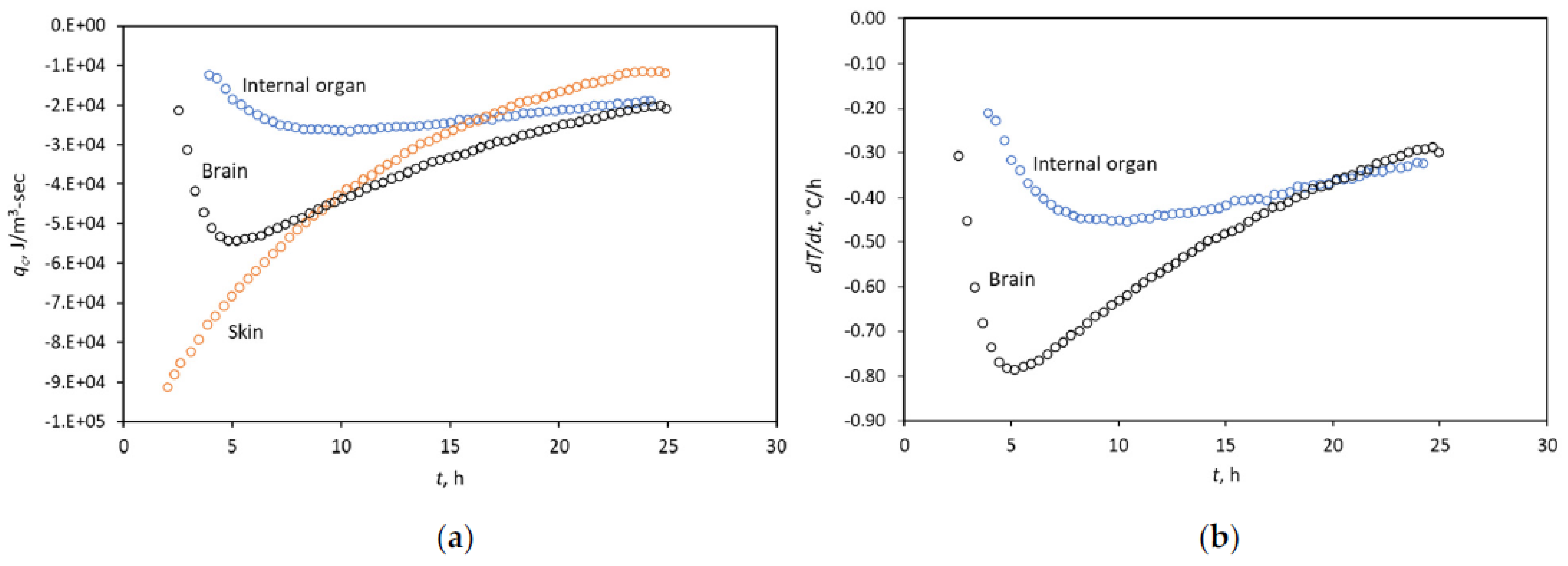
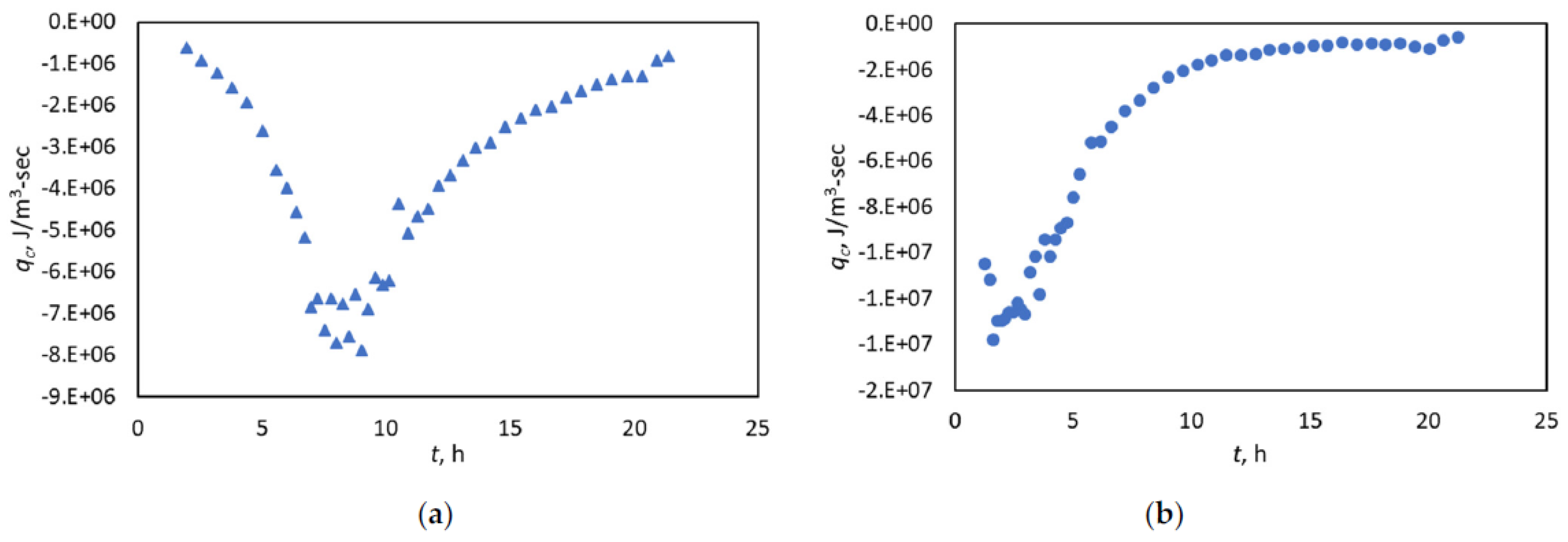
3.2. Diagnosing the Fitting Window with the Heat-Flow Rate
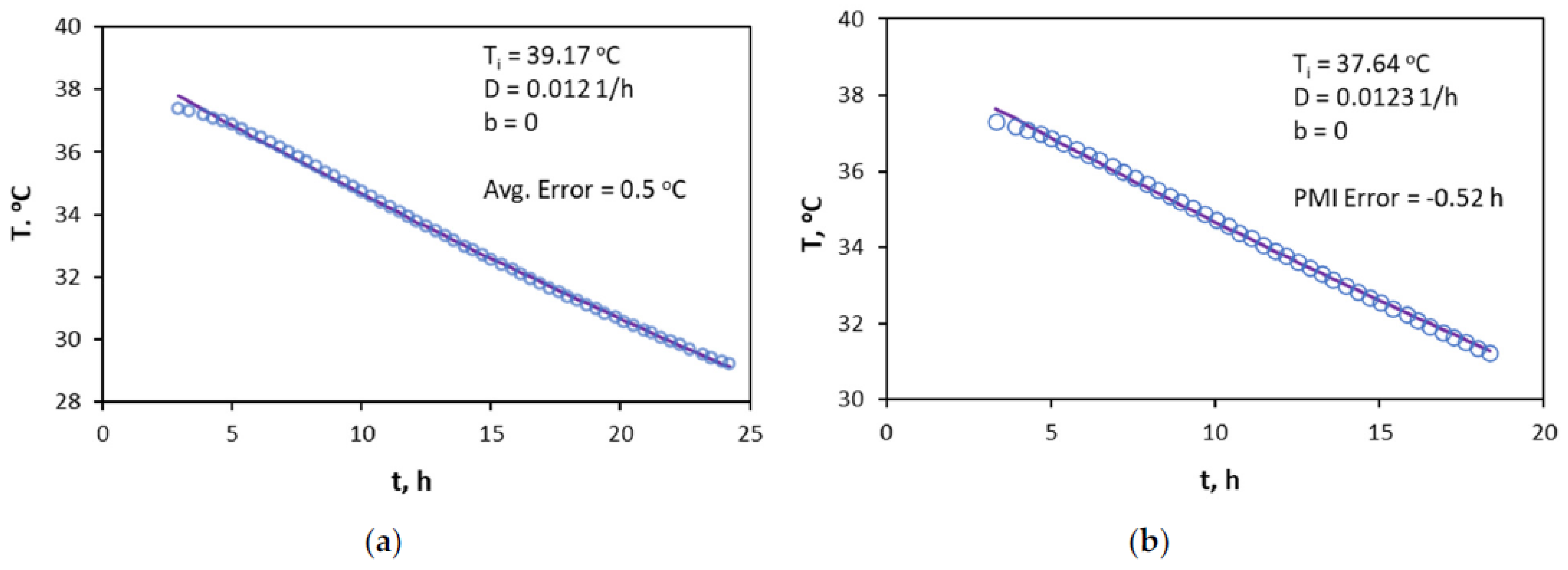
3.3. Application of the Hyperbolic Approach for PMI Estimation
4. Discussion
5. Conclusions
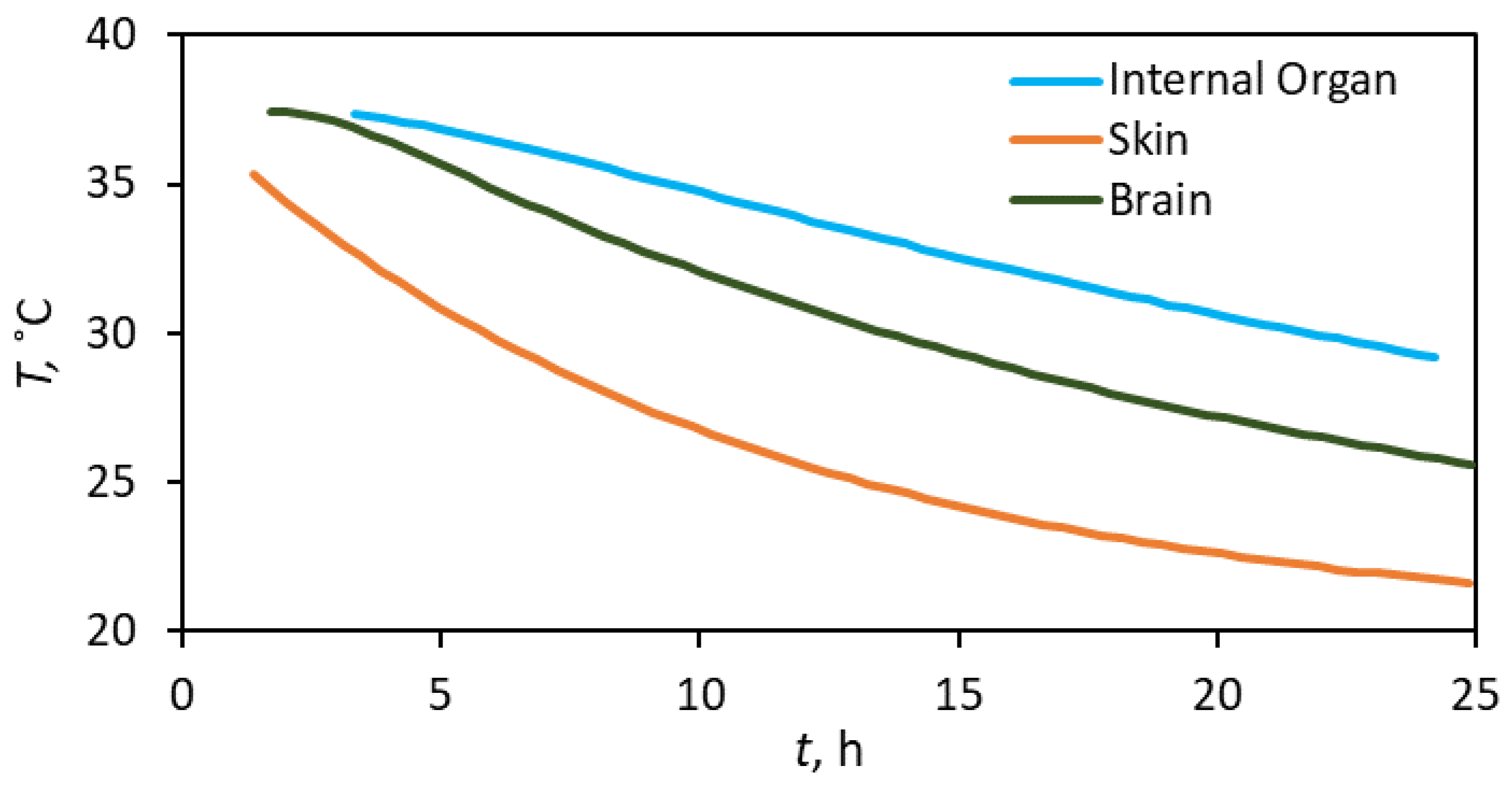
- A rapid temperature decline rate occurs initially, followed by a slower pace, regardless of the body part. Therefore, the hyperbolic trend can describe the overall signature. As part of the general hyperbolic trend, the exponential decay may represent some aspects of the overall signature, but it does not appear systemic. Stated differently, the application of Newton’s law of cooling does not appear holistic in the body-temperature decline.
- Ascertaining the PMI from a single-temperature data point appears challenging. Knowing both the initial body temperature and that of the room does not suffice, given that the cooling constant, kc, is dependent on an individual’s body characteristics and surrounding conditions. In other words, gathering time-lapse data appears a requirement for a reliable solution for estimating PMI.
- The hyperbolic relation fits all monotonic trends, established either by temperature derivative or the heat-flow rate, regardless of the body part. This fitting leads to a high degree of PMI accuracy, that is, 0.24 h on average for the cases reported in this study.
Supplementary Materials
Author Contributions
Funding
Institutional Review Board Statement
Informed Consent Statement
Data Availability Statement
Conflicts of Interest
Nomenclature
| b | time-derivative of D in Arps, dimensionless |
| Ct | heat capacity of tissue, J/kg-°C |
| D | log-time derivative of temperature in Arps, 1/h |
| kc | cooling constant, 1/h |
| qc | heat-flow rate, J/m3.sec |
| t | time, h |
| T | temperature, °C |
| Ta | ambient temperature, °C |
| Ti | initial temperature at time of death, °C |
| dT/dt | temperature gradient, °C/h |
| ρt | density of tissue, kg/m3 |
Appendix A
Estimating the Cooling Constant with Limited Data

| Time of Death | 8:30:00 a.m. |
|---|---|
| Temperature at time of death (Ti) | 38.22 °C |
| Ambient Temperature (Ta) | 30.61 °C |
| Temperature at 12 a.m. | 36.61 °C |
| Temperature at 1 PM | 36.17 °C |
| Temperature at 2 PM | 35.83 °C |
| Time Interval | kc (1/h) | Estimated PMI (h) | Actual PMI (h) | Difference (min) |
|---|---|---|---|---|
| 12 a.m.–1 p.m. | 0.07696 | 3.09 | 3.5 | 25 |
| 1 p.m.–2 p.m. | 0.061875 | 3.84 | 3.5 | −21 |
| 12 a.m.–2 p.m. | 0.069418 | 3.43 | 3.5 | 4 |
| Avg (12 a.m.–1 p.m.) and (1 p.m.–2 p.m.) | 0.069418 | 3.40 | 3.5 | 4 |
| Time Interval | kc (1/h) | Estimated PMI (h) | Actual PMI (h) | Difference (min) |
|---|---|---|---|---|
| 2 to 4 h | 0.05 | 2.19 | 2.13 | −4 |
| 2 to 6 h | 0.05 | 2.21 | 2.13 | −5 |
| Time Interval | kc (1/h) | Estimated PMI (h) | Actual PMI (h) | Difference (min) |
|---|---|---|---|---|
| 1 to 2 h | 0.17 | 0.80 | 1.20 | 24 |
| 1 to 4 h | 0.15 | 0.94 | 1.20 | 15 |
| 1 to 5 h | 0.14 | 1.02 | 1.20 | 11 |
References
- Rainy, H. On the cooling of dead bodies as indicating the length of time since death. Glasg. Med. J. 1968, 1, 323–330. [Google Scholar]
- Kaliszan, M.; Hauser, R.; Kaliszan, R.; Wiczling, P.; Buczyñski, J.; Penkowski, M. Verification of the exponential model of body temperature decrease after death in pigs. Exp. Physiol. 2005, 90, 727–738. [Google Scholar] [CrossRef] [PubMed]
- Noakes, L.D.; Flint, T.; Williams, J.H.; Knight, B.H. The application of eight reported temperature-based algorithms to calculate the postmortem interval. Forensic Sci. Int. 1992, 54, 109–125. [Google Scholar] [CrossRef]
- De Saram, G.; Webster, G.; Kathirgamatamby, N. Post-mortem temperature at time of death. J. Crim. Law Criminol. Police Sci. 1955, 46, 562–577. [Google Scholar] [CrossRef]
- Fiddes, F.; Patten, T.A. Percentage method for representing the fall in body temperature. J. Forensic Med. 1958, 5, 2–15. [Google Scholar]
- Marshall, T.K.; Hoare, F. Estimating the time since death—The rectal cooling after death and its mathematical representation. J. Forensic Sci. 1962, 7, 56–81. [Google Scholar]
- Al-Alousi, L.M.; Anderson, R.A. A non-invasive method for postmortem temperature measurements using a microwave probe. Forensic Sci. Int. 1994, 64, 35–46. [Google Scholar] [CrossRef]
- Green, M.; Wright, J. Postmortem interval estimation from body temperature data only. Forensic Sci. Int. 1985, 28, 35–46. [Google Scholar] [CrossRef]
- Henssge, C. Death time estimation in case work. I. The rectal temperature time of death nomogram. Forensic Sci. Int. 1988, 36, 209–236. [Google Scholar] [CrossRef]
- Marshall, T.K. Estimating the time of death. J. Forensic Sci. 1962, 7, 210–221. [Google Scholar]
- Marshall, T.K. Temperature methods of estimating the time of death. Med. Sci. Law 1965, 4, 224–232. [Google Scholar] [CrossRef] [PubMed]
- Al-Alousi, L.M.; Anderson, R.A.; Worster, D.M.; Land, D.V. Factors influencing the precision of estimating the postmortem interval using the triple-exponential formulae (TEF) Part I. A study of the effect of body variables and covering of the torso on the postmortem brain, liver and rectal cooling rates in 117 forensic cases. Forensic Sci. Int. 2002, 125, 223–230. [Google Scholar] [PubMed]
- Al-Alousi, L.M.; Anderson, R.A.; Worster, D.M.; Land, D.V. Factors influencing the precision of estimating the postmortem interval using the triple-exponential formulae (TEF) Part II. A study of the effect of body temperature at the moment of death on the postmortem brain, liver and rectal cooling rates in 117 forensic cases. Forensic Sci. Int. 2002, 125, 231–236. [Google Scholar] [CrossRef] [PubMed]
- Mall, G.; Eisenmenger, W. Estimation of time since death by heat-flow Finite-Element model. Part I: Method, model, calibration and validation. Leg. Med. 2005, 7, 1–14. [Google Scholar] [CrossRef] [PubMed]
- Mall, G.; Eisenmenger, W. Estimation of time since death by heat-flow Finite-Element model. Part II: Application to non-standard cooling conditions and preliminary results in practical casework. Leg. Med. 2005, 7, 69–80. [Google Scholar] [CrossRef]
- Rodrigo, M.R. Time of death estimation from temperature readings only: A Laplace transform approach. Appl. Math Lett. 2015, 39, 47–52. [Google Scholar] [CrossRef]
- Smart, J.L. Estimation of time of death with a Fourier series unsteady-state heat transfer model. J. Forensic Sci. 2010, 55, 1481–1487. [Google Scholar] [CrossRef]
- Baccino, E.; Martin, L.D.S.; Schuliar, Y.; Guilloteau, P.; Rhun, M.L.; Morin, J.F.; Leglise, D.; Amice, J. Outer ear temperature and time of death. Forensic Sci. Int. 1996, 83, 133–146. [Google Scholar] [CrossRef]
- Smart, J.L.; Kaliszan, M. The postmortem temperature plateau and its role in the estimation of time of death. A review. Leg. Med. 2012, 14, 55–62. [Google Scholar] [CrossRef]
- Kaliszan, M. First practical applications of eye temperature measurements for estimation of time of death in casework. Report of three cases. Forensic Sci. Int. 2012, 219, e13–e15. [Google Scholar] [CrossRef]
- Kaliszan, M. Studies on time of death estimation in the early postmortem period—Application of a method based on eyeball temperature measurement to human bodies. Leg. Med. 2013, 15, 278–282. [Google Scholar] [CrossRef] [PubMed]
- Kaliszan, M.; Wujtewicz, M. Eye temperature measured after death in human bodies as an alternative method of time of death estimation in the early postmortem period. A successive study on new series cases with exactly known time of death. Leg. Med. 2019, 38, 10–13. [Google Scholar] [CrossRef] [PubMed]
- Nelson, E.L. Estimation of short-term postmortem interval utilizing core body temperature: A new algorithm. Forensic Sci. Int. 2000, 109, 31–38. [Google Scholar] [CrossRef]
- Laplace, K.; Baccino, E.; Peyron, P.-A. Estimation of the time since death based on body cooling: A comparative study of four-temperature based models. Int. J. Leg. Med. 2021, 135, 2479–2487. [Google Scholar] [CrossRef]
- Baccino, E.; Cattaneo, C.; Jouineau, C.; Poudoulec, J.; Martrille, L. Cooling rates of the ear and brain in pig heads submerged in water: Implications for postmortem interval estimation of cadavers found in still water. Am. J. Forensic Med. Pathol. 2007, 28, 80–85. [Google Scholar] [CrossRef]
- Napoli, P.E.; Nioi, M.; Gabiati, L.; Laurenzo, M.; De-Giorgio, F.; Scorcia, V.; Grassi, S.; d’Aloja, E.; Fossarello, M. Repeatability and reproducibility of postmortem central corneal thickness measurements using a portable optical coherence tomography system in humans: A prospective multicenter study. Sci. Rep. 2020, 10, 14508. [Google Scholar] [CrossRef]
- Locci, E.; Stocchero, M.; Noto, A.; Chighine, A.; Natali, L.; Napoli, P.E.; Caria, R.; De-Giorgio, F.; Nioi, M.; D’Aloja, E. A 1H NMR metabolomic approach for the estimation of the time since death using aqueous humour: An animal model. Metabolomics 2019, 15, 76. [Google Scholar] [CrossRef]
- Locci, E.; Stocchero, M.; Gottardo, R.; De-Giorgio, F.; Demontis, R.; Nioi, M.; Chighine, A.; Tagliaro, F.; D’Aloja, E. Comparative use of aqueous humour 1H NMR metabolomics and potassium concentration for PMI estimation in an animal model. Int. J. Leg. Med. 2021, 135, 845–852. [Google Scholar] [CrossRef]
- Zilg, B.; Alkass, K.; Berg, S.; Druid, H. Interpretation of postmortem vitreous concentrations of sodium and chloride. Forensic Sci. Int. 2016, 263, 107–113. [Google Scholar] [CrossRef]
- Bartgis, C.; LeBrun, M.; Ma, R.; Zhu, L. Determination of time of death in forensic science via a 3-D whole body heat transfer model. J. Therm. Biol. 2016, 62, 109–115. [Google Scholar] [CrossRef]
- Sharma, P.; Al Saedi, A.; Kabir, C.S. Assessing the hyperbolic trend in well response involving pressure, fluid and heat-flow rates. J. Nat. Gas Sci. Eng. 2020, 78, 103292. [Google Scholar] [CrossRef]
- Lyle, H.; Cleveland, F. Determination of the time of death by heat loss. J. Forensic Sci. 1956, 1, 11–24. [Google Scholar]
- Kanawaku, Y.; Kanetake, J.; Komiya, A.; Maruyama, S.; Funayama, M. Computer simulation for post-mortem cooling process in the outer ear. Leg. Med. 2007, 9, 55–62. [Google Scholar] [CrossRef] [PubMed]
- Wilk, L.S.; Hoveling, R.J.M.; Edelman, G.J.; Hardy, H.J.J.; van Schouwen, S.; van Venrooij, H.; Aalders, M.C.G. Reconstructing the time since death using noninvasive thermometry and numerical analysis. Sci. Adv. 2020, 6, eaba4243. [Google Scholar] [CrossRef]
- Wilk, L.S.; Edelman, G.J.; Roos, M.; Clerkx, M.; Dijkman, I.; Melgar, J.V.; Oostra, R.-J.; Aalders, M.C.G. Individualised and non-contact postmortem interval determination of human bodies using visible and thermal 3D imaging. Nat. Commun. 2021, 12, 5997. [Google Scholar] [CrossRef]


| Source | Body Part | Start of Fitting Window, h | Estimated PMI, h | Actual PMI, h | ΔPMI, h | b-Factor, Dimensionless | D, 1/h |
|---|---|---|---|---|---|---|---|
| Bertgis et al. | Internal Organ | 3 | 2.8 | 3.3 | 0.5 | 0 | 0.012 |
| Bertgis et al. | Internal Organ | 5 | 3.7 | 5.0 | 1.3 | 0 | 0.012 |
| Bertgis et al. | Internal Organ | 9 | 8.2 | 9.3 | 1.2 | 0 | 0.012 |
| Bertgis et al. | Brain | 3 | 3.8 | 3.3 | −0.5 | 0 | 0.017 |
| Bertgis et al. | Brain | 5 | 5.8 | 5.2 | −0.6 | 0 | 0.017 |
| Bertgis et al. | Brain | 9 | 10.1 | 9.3 | −0.8 | 0 | 0.017 |
| Wilk et al. | Case B-Abdomen | 3 | 3.2 | 3.5 | 0.3 | 8.5 | 0.032 |
| Wilk et al. | Case B-Abdomen | 5 | 5.3 | 5.6 | 0.3 | 8.5 | 0.020 |
| Wilk et al. | Case B-Abdomen | 9 | 10.0 | 9.7 | −0.3 | 8.1 | 0.012 |
| Wilk et al. | Case B-Forehead | 3 | 3.6 | 3.1 | −0.5 | 5.3 | 0.039 |
| Wilk et al. | Case B-Forehead | 5 | 5.4 | 5.6 | 0.2 | 5.8 | 0.027 |
| Wilk et al. | Case B-Forehead | 9 | 7.8 | 9.4 | 1.6 | 6.7 | 0.018 |
| Wilk et al. | Case B-Thighs | 3 | 5.1 | 3.0 | −2.1 | 4.5 | 0.030 |
| Wilk et al. | Case B-Thighs | 5 | 6.7 | 5.1 | −1.6 | 4.7 | 0.024 |
| Wilk et al. | Case B-Thighs | 9 | 8.8 | 9.9 | 1.1 | 6.1 | 0.017 |
| Wilk et al. | Case B-Chest | 3 | 3.2 | 3.1 | −0.1 | 10 | 0.028 |
| Wilk et al. | Case B-Chest | 5 | 5.1 | 5.2 | 0.1 | 10 | 0.018 |
| Wilk et al. | Case B-Chest | 9 | 9.5 | 9.4 | 0.0 | 10 | 0.010 |
| Wilk et al. | Case C-Forehead | 3 | 2.1 | 3.3 | 1.2 | 10 | 0.046 |
| Wilk et al. | Case C-Forehead | 5 | 5.4 | 5.2 | −0.2 | 10 | 0.018 |
| Wilk et al. | Case C-Abdomen | 9 | 10.8 | 10.0 | −0.8 | 5 | 0.014 |
| Wilk et al. | Case D-Forehead | 3 | 3.1 | 4.2 | 1.1 | 10 | 0.032 |
| Wilk et al. | Case D-Forehead | 5 | 5.1 | 5.6 | 0.5 | 10 | 0.019 |
| Wilk et al. | Case D-Abdomen | 3 | 2.9 | 3.5 | 0.6 | 9.11 | 0.034 |
| Wilk et al. | Case D-Abdomen | 5 | 5.8 | 6.5 | 0.8 | 9.17 | 0.018 |
| Wilk et al. | Case D-Abdomen | 9 | 8.5 | 9.4 | 0.9 | 9.1 | 0.012 |
Publisher’s Note: MDPI stays neutral with regard to jurisdictional claims in published maps and institutional affiliations. |
© 2022 by the authors. Licensee MDPI, Basel, Switzerland. This article is an open access article distributed under the terms and conditions of the Creative Commons Attribution (CC BY) license (https://creativecommons.org/licenses/by/4.0/).
Share and Cite
Sharma, P.; Kabir, C.S. A Simplified Approach to Understanding Body Cooling Behavior and Estimating the Postmortem Interval. Forensic Sci. 2022, 2, 403-416. https://doi.org/10.3390/forensicsci2020030
Sharma P, Kabir CS. A Simplified Approach to Understanding Body Cooling Behavior and Estimating the Postmortem Interval. Forensic Sciences. 2022; 2(2):403-416. https://doi.org/10.3390/forensicsci2020030
Chicago/Turabian StyleSharma, Pushpesh, and C. S. Kabir. 2022. "A Simplified Approach to Understanding Body Cooling Behavior and Estimating the Postmortem Interval" Forensic Sciences 2, no. 2: 403-416. https://doi.org/10.3390/forensicsci2020030
APA StyleSharma, P., & Kabir, C. S. (2022). A Simplified Approach to Understanding Body Cooling Behavior and Estimating the Postmortem Interval. Forensic Sciences, 2(2), 403-416. https://doi.org/10.3390/forensicsci2020030