Comparative Analysis of Throughput Prediction Models in SAG Mill Circuits: A Geometallurgical Approach

Abstract

This study was conducted on a copper porphyry deposit located in Espinar, Cusco (Peru), with the objective of developing and comparing predictive models for processing capacity in SAG grinding circuits. A total of 174 samples were used for the JK Drop Weight Test (JKDWT) and 1172 for the Bond Work Index (BWi), along with 36 months of operational plant data. Three modeling methodologies were evaluated: DWi-BWi, SGI-BWi, and SMC-BWi (Mia, Mib), all integrated into a geometallurgical block model. Validation was performed through reconciliation with actual plant data, considering operational constraints such as transfer size (T₈₀) and maximum throughput (TPH). The model based on SMC parameters and BWi showed the best predictive performance, with a root mean square error (RMSE) of 143 t/h and a mean relative deviation of 1.5%. This approach enables more accurate throughput forecasting, improving mine planning and operational efficiency. The results highlight the importance of integrating geometallurgical and operational data to build robust models that are adaptable to ore variability and applicable to both short- and long-term planning scenarios.

1. Introduction

In recent years, the copper industry has faced significant productivity challenges due to declining ore grades and rising operational costs, particularly those associated with energy consumption. A notable example is the Antapaccay plant, which reported an energy consumption of 0.85 TWh in 2024 [1]. These factors have necessitated more rigorous planning in both ore extraction and processing [2]. Effective modeling of comminution processes is critical to the success of mining operations, as inadequate control can hinder the liberation of valuable minerals, leading to losses in downstream recovery stages [3].

Ore hardness is an intrinsic property of the deposit and, therefore, cannot be directly controlled by plant operators. When the ore exhibits higher resistance to breakage, the size reduction process slows down, increasing the internal load of the mill under constant feed conditions [4]. In scenarios where the mill operates below its nominal capacity, this increased load results in higher energy consumption per ton processed, as more energy is required to achieve the same degree of mineral liberation [5]. Conversely, if the mill is already operating at full capacity, an increase in ore hardness may lead to overloading, a condition that can only be mitigated by reducing the feed rate [6]. This behavior has been extensively documented in studies on energy efficiency and load dynamics in SAG mills, which emphasize the importance of adjusting operational parameters such as mill speed, filling level, and grinding media ratio to maintain optimal performance [7].

Recent research has also shown that variability in ore hardness can induce operational instability, affecting product size distribution and bearing pressure within the mill [8]. To address these challenges, dynamic simulation models have been developed to predict mill behavior in response to changes in ore hardness, enabling the implementation of adaptive control strategies [9]. Additionally, the design and optimization of internal mill liners—such as trapezoidal liners—play a significant role in process efficiency by altering the trajectory of grinding media and their impact on the ore [10,11].

The comminution circuit at the Antapaccay plant consists of a primary crusher followed by a grinding line, which includes a 24,000 kW semi-autogenous (SAG) mill feeding two ball mills with a combined power of 32,800 kW, and a pebble crushing circuit. The total system throughput, typically limited by hydraulic transport conditions, is 4058 t/h. The current product from the grinding circuit has a maximum transfer size (T₈₀max) of 19,783 microns between the SAG and ball grinding stages, and a P₈₀ (80% passing) of 228 microns [12].

In general, the modeling of SABC circuits (SAG mill, ball mill, and pebble crushing) for geometallurgical purposes is based on laboratory test results that capture the spatial variability of comminution attributes [13,14]. At Minera Antapaccay, the JK Drop Weight Test (JKDWT) [15,16] and the Bond Ball Mill Work Index (BWi) [17] are used. These tests support the development of performance models based on specific energy consumption relationships [18,19]. Furthermore, recent innovations in SAG mill design have been reported [20].

The geometallurgical performance model is updated annually through a structured sequence of activities designed to maintain predictive accuracy in the face of deposit variability. This process includes selection of variability samples using standard-length drill cores representative of different zones within the deposit [21]; determination of comminution indices such as the Bond Work Index and the Abrasion Index from the collected samples [19]; quality control of the generated databases, followed by estimation of comminution variables at the geometallurgical block model level using geostatistical techniques [20]; transformation of interpolated comminution indices into performance estimates using process models previously calibrated with historical operational data [22]; and reconciliation of the performance model with metallurgical accounting data, enabling the identification of deviations and model adjustments [23]. This reconciliation also supports the definition of key performance indicators (KPIs) to assess model accuracy and reliability [24].

This study presents the development and evaluation of three geometallurgical performance model alternatives, aiming to identify the one that best represents ore throughput at Minera Antapaccay [7]. These models are designed to support mine planning and project development across short-, medium-, and long-term horizons, as well as to meet specific operational requirements [25,26,27].

The three proposed alternatives are based on different sets of comminution parameters widely used in the mining industry to model ore behavior in grinding processes:

• Model based on the Bond Work Index (BWi) and the Drop Weight Index (DWi) [28],
• Model based on SMC indices (Mia, Mib) and BWi tests [29], and
• Model based on the SAG Grindability Index (SGI) and BWi [19,20].

The most suitable model is selected based on its predictive accuracy against historical operational data and its consistency with metallurgical reconciliation results [30]. This approach reduces uncertainty in mine planning and enhances strategic decision making [31].

Numerous studies have demonstrated the value of site-specific throughput models in improving operational predictability and reducing processing variability. Daniel and Wang highlighted the benefits of developing customized SAG mill throughput forecast models for gold, copper, and iron ore concentrators, emphasizing that once in operation, most variables in the SAG-specific energy equation remain constant, making ore competency (DWi) the dominant factor influencing throughput [32]. Similarly, Both and Dimitrakopoulos developed a machine learning-based geometallurgical throughput model at the Tropicana Gold Mine, showing that integrating hardness proxies and circuit variables significantly improved prediction accuracy [33]. Additionally, Bueno et al. demonstrated how geometallurgical modeling applied to comminution can reduce design risks and improve throughput forecasting by incorporating spatial variability into early-stage mine planning [34].

This work contributes to the field by systematically comparing multiple throughput modeling approaches under real operational conditions, integrating geometallurgical block models with plant reconciliation data. Unlike previous studies, it emphasizes the practical implementation of these models in a high-throughput copper operation, offering a robust and transferable methodology for improving throughput prediction and supporting strategic decision making in complex ore environments.

2. Materials and Methods

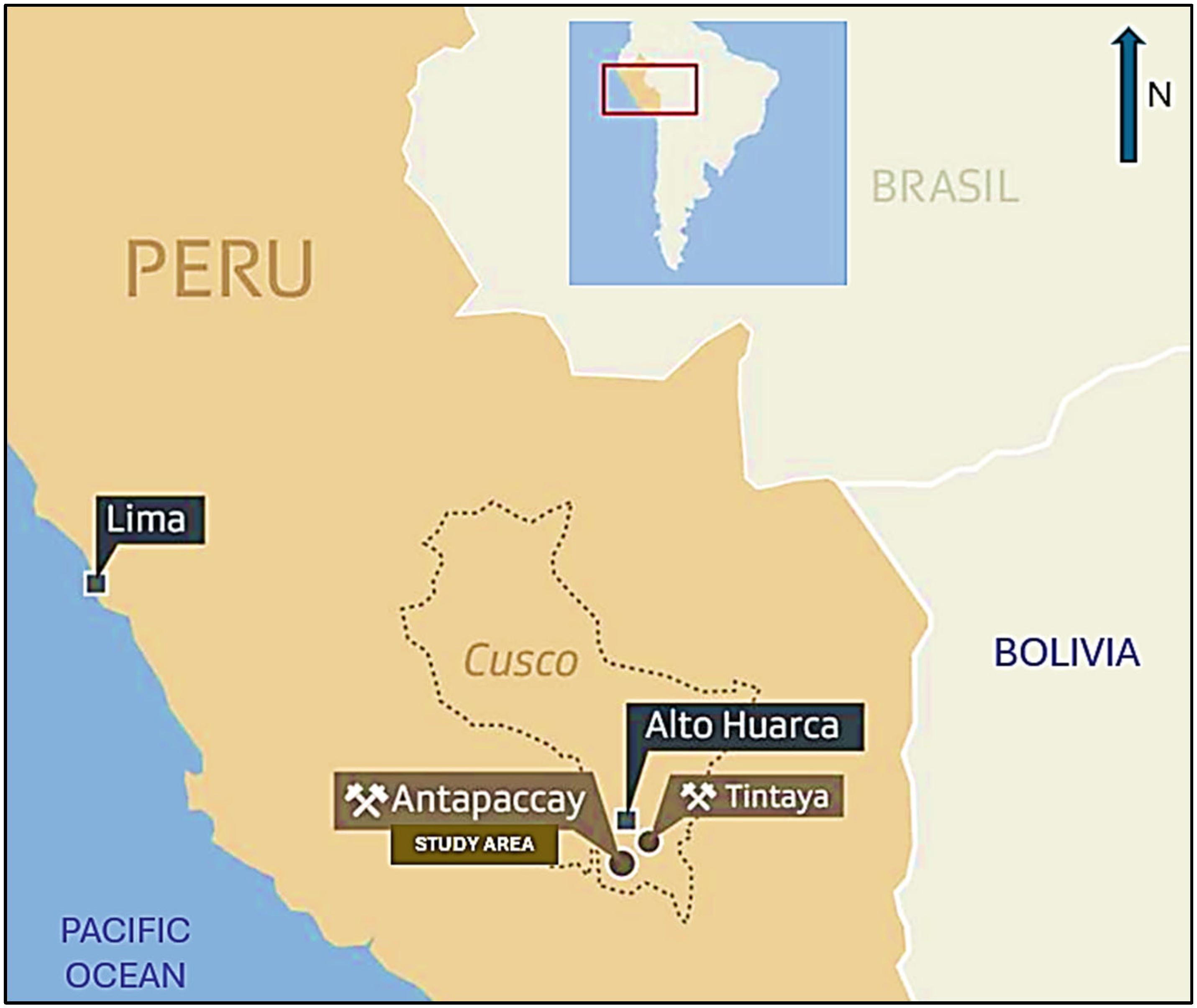
The study area is located approximately 12 km in a straight line southwest of the Tintaya mine, within the Alto Huarca rural community, Espinar district and province, Cusco department, in southeastern Peru (Figure 1). Mining activities in this area are carried out using the open-pit method, commonly applied to porphyry-skarn type deposits [30,31].

Geologically, the deposit is part of the Eocene–Oligocene metallogenic belt of the Andahuaylas-Yauri magmatic arc, a region known for its diversity of mineral deposits such as Las Bambas, Los Quechuas, Los Chancas, Antilla, Trapiche, Haquira, and the Antapaccay expansion with the Coroccohuayco project [35,36].

The local geological units include the Maras and Ferrobamba formations, from the Lower and Upper Cretaceous, respectively. These formations have undergone intense folding during Andean tectonic events and were later intruded by stocks, sills, and dikes of the Andahuaylas-Yauri Batholith [37,38,39]. The overlying cover consists of Miocene lacustrine and volcanic deposits, as well as more recent Quaternary deposits [39].

Regarding hydrothermal alteration, three main types have been identified: potassic (potassium feldspar and quartz veinlets), phyllic (quartz-sericite-pyrite), and propylitic (chlorite veinlets), which are typical of porphyry-skarn systems [39,40,41].

Copper mineralization is primarily hosted in intermediate intrusive rocks such as diorite and monzonite, as well as in veinlets, hydrothermal breccias, and contacts with sedimentary rocks (limestones, calcareous shales, siltstones, and sandstones), forming contact breccias, skarn-type bodies, and stockwork structures [35,36,41].

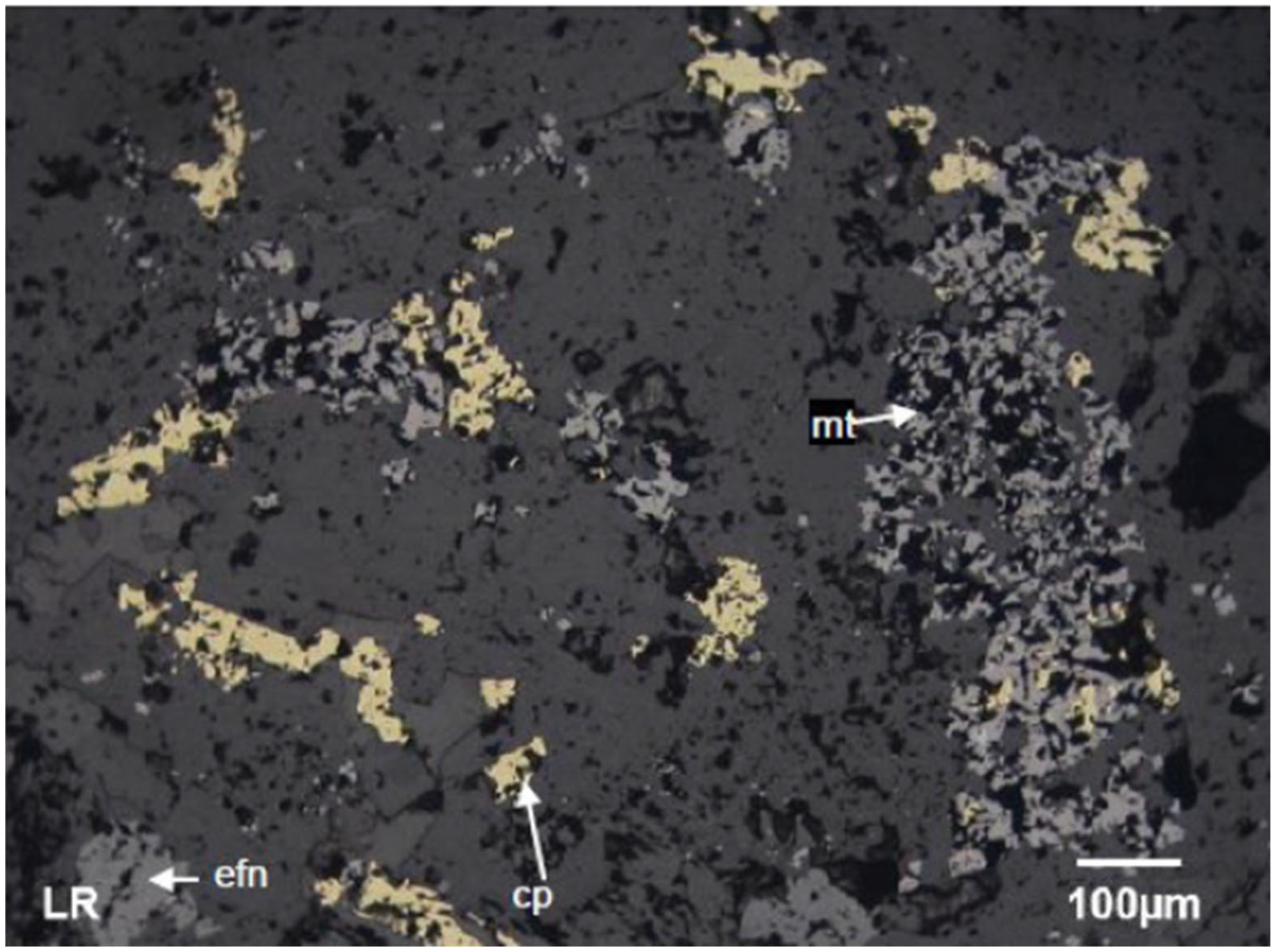
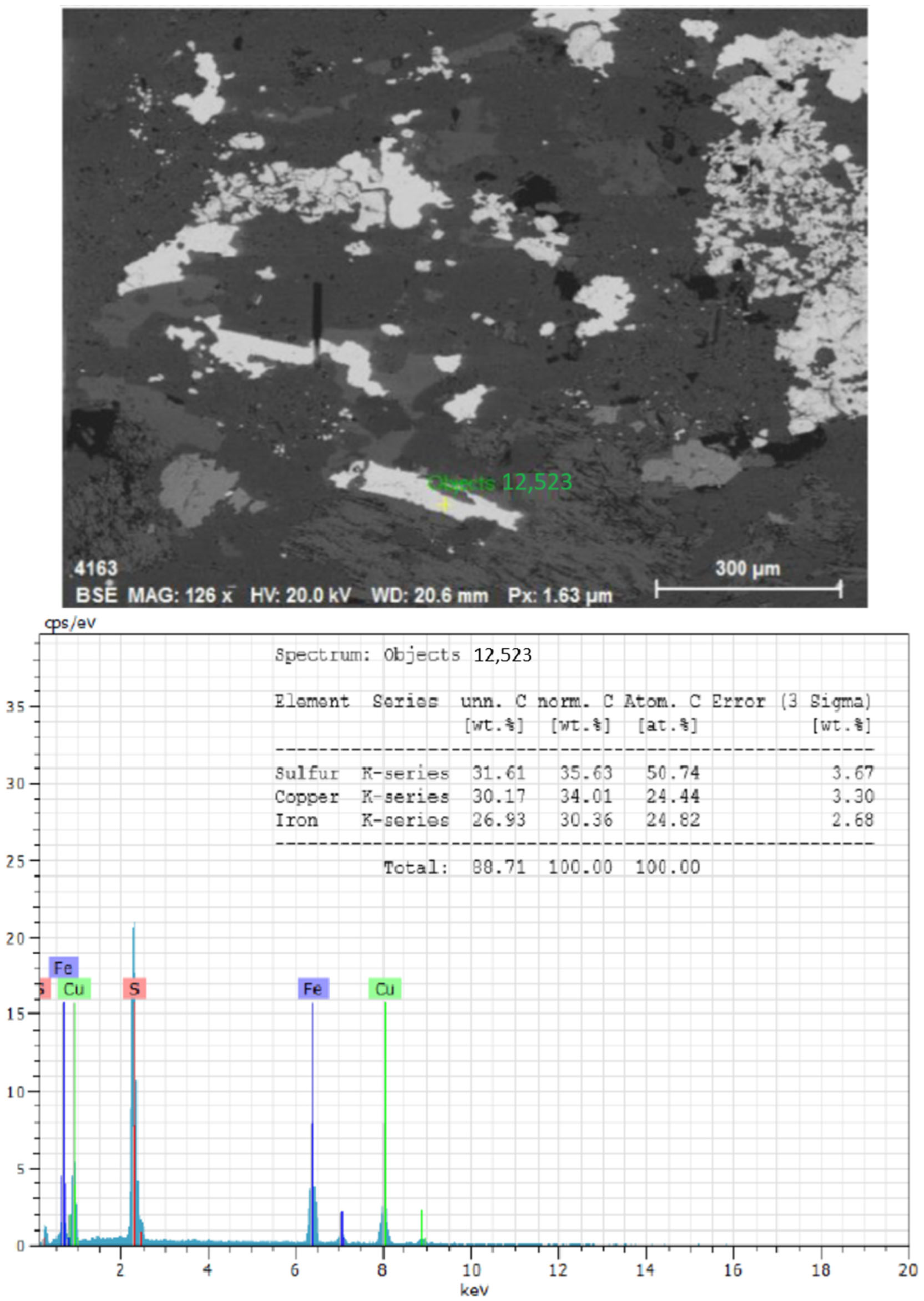
The mineralogy is dominated by chalcopyrite, with contents up to 3.4%, surpassing bornite in the upper zones. At greater depths, this relationship reverses, and mineralization is associated with anhydrite and gypsum levels [42,43,44,45]. Appendix B.

Two main mineralized bodies have been identified: the southern body, extending 1300 m in a NW–SE direction with a variable width between 250 and 430 m; and the northern body, 300 m long and 450 m wide [30].

The contact between intrusions and host rocks has generated a skarn facilitated by quartz metasomatism, creating favorable conditions for stockwork development. This stockwork is structurally controlled by regional faults affecting the intrusive-sedimentary complex, enabling mineral dissemination. Additionally, stockwork zones controlled by local faults have been identified [37,45,46].

The concentrator plant operated by Antapaccay mining company is equipped with a “60 × 113” primary gyratory crusher, designed to process up to 7500 tons of ore per hour, reducing its size to approximately 178 mm [47]. The ore is then transported via a 7-km conveyor belt to a 40 × 26-foot semi-autogenous grinding (SAG) mill powered by a 24 MW motor. This mill features a short trommel and a vibrating screen, feeding two 26 × 40.5-foot ball mills, each with an installed power of 16.4 MW [47]. The system operates in a reverse closed circuit, which includes three batteries composed of 13 cyclones each, with a diameter of 33, as illustrated in Figure 2 [47].

For this study, operational data collected from the plant over the past 36 months will be used. To ensure data quality and consistency, only days when the SAG mill operated for more than 22.8 h (at least 95% of the day) will be considered. Likewise, only months with more than 80% of days under stable operating conditions will be included. Applying these filtering criteria, 30 valid months have been identified for the reconciliation analysis

Table 1. Calculated Data for Model Reconciliation.

Month	Year	SAG F80 (µm)	SAG TPH
1	1	73,427	3734
2	1	76,547	3628
3	1	73,245	3765
4	1	77,474	3549
5	1	71,273	4058
6	1	74,567	3927
7	1	72,345	3789
8	1	76,543	3654
9	1	73,456	3745
10	1	75,432	3897
11	1	72,345	3765
12	1	76,543	3654
1	2	73,427	3734
2	2	76,547	3628
3	2	73,245	3765
4	2	77,474	3549
5	2	71,273	4058
6	2	74,567	3927
7	2	72,345	3789
8	2	76,543	3654
9	2	73,456	3745
10	2	75,432	3897
11	2	72,345	3765
12	2	76,543	3654
1	3	73,427	3734
2	3	76,547	3628
3	3	73,245	3765
4	3	77,474	3549
5	3	71,273	4058
6	3	74,567	3927
7	3	72,345	3789
8	3	76,543	3654
9	3	73,456	3745
10	3	75,432	3897
11	3	72,345	3765
12	3	76,543	3654

.

A cut-off grade of 0.1% Cu has been established, used as a criterion to filter only those blocks considered economically viable, in accordance with the Resources and Reserves report. For ore characterization, 158 samples corresponding to the A×b parameter and 1172 samples associated with the Bond Work Index (BWi) are available.

The following information sources will be used in this study:

• PI system records containing operational variables from the comminution circuit.
• Database with results from the JK Drop Weight Test (JKDWT).
• Database with the Bond Work Index (BWi) values.
• Block model identifying the ore units extracted and processed during the analysis period.
• Geometallurgical block model used to estimate processing capacity.

Preliminary analysis of these data allows for proper configuration of input variables, detection of atypical operating periods, and establishment of criteria to define the validity of days or months included in the model comparison. From the selected periods, the necessary variables are calculated for calibration and evaluation of each model considered.

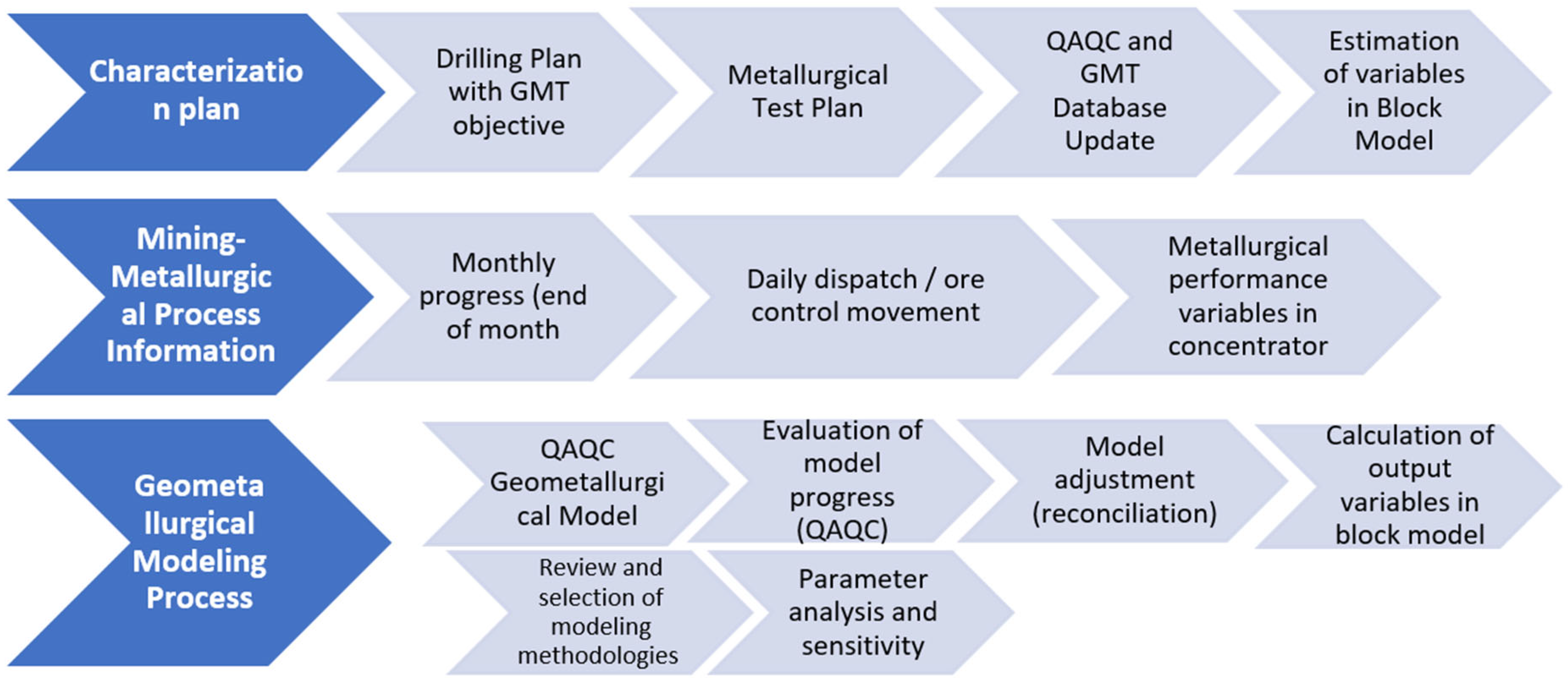
2.1. Integrated Workflow for Mining, Metallurgical Data Management, and Geometallurgical Modeling

The development of the comminution model follows a structured sequence encompassing: the characterization plan, collection of mining-metallurgical process data, and geometallurgical modeling (see Figure 3).

• Characterization Plan:
  This stage involves designing drilling campaigns from which samples are obtained for metallurgical testing. After rigorous quality control (QA/QC), the results are incorporated into the block model through geostatistical estimation processes.
• Mining-Metallurgical Process Data:
  Using data from monthly closing reports and daily operation logs, filtering is performed to identify ideal processing conditions. Only days with more than 22.8 h of SAG mill operation (95% of the day) and months with over 80% stable days are considered valid. Raw data are extracted from the PI system and cleaned to remove inconsistencies or measurement errors (Appendix A).
• Geometallurgical Modeling:
  In this phase, files with the required variables are prepared and formatted according to procedural guidelines. The information is cleaned, and calculations are performed to reconcile the processing model with operational data. The quality of the geometallurgical model is evaluated, including mining progress in the block model, and adjusted using different approaches: the model based on DWi and BWi, the Morrell power model, and the model using SGI and BWi. The equations used to transform A×b and BWi results into the various comminution indices employed in this study are also presented [48,49]. Additionally, grinding circuit optimization has been considered as part of the analysis [50].

2.2. The JKMRC Drop Weight Impact Breakage Test

Sample requirements: The test requires an initial sample of approximately 100 kg, with particle sizes between −63 and 13.2 mm [51].

Outputs: The test delivers the specific energy consumption Ecs (kWh/t) and the parameters (A, b) that represent mineral fracture behavior.

Equation: The latter are calculated by adjusting the data of t₁₀ and Ecs according to the following equation [52]:

$$t_{10}=A\cdot \left[1-e^{\left(-b\cdot Ecs\right)}\right]$$

(1)

where

• A represents the maximum curvature, and
• b defines the shape of the curve as it approaches the upper limit.

These parameters indicate the natural breakage limit of the rock and the rate at which the rock reaches this maximum, respectively.

Parameters A and b are not independent, so they cannot be used directly to make comparisons between mineral types; on the other hand, the product A×b is an alternative that allows a direct comparison [14].

This

Table 2. Descriptive Statistics of the A×b Breakage Parameter for Geometallurgical Characterization.

	A×b
Count	174
Average	51.2
SD	18.6
Min	25
Max	139

summarizes the descriptive statistics of the A×b parameter, which characterizes ore breakage behavior in geometallurgical modeling. The values represent the distribution of A×b across 174 samples, providing insight into the variability of ore hardness within the deposit. These metrics are essential for calibrating comminution models and optimizing processing strategies

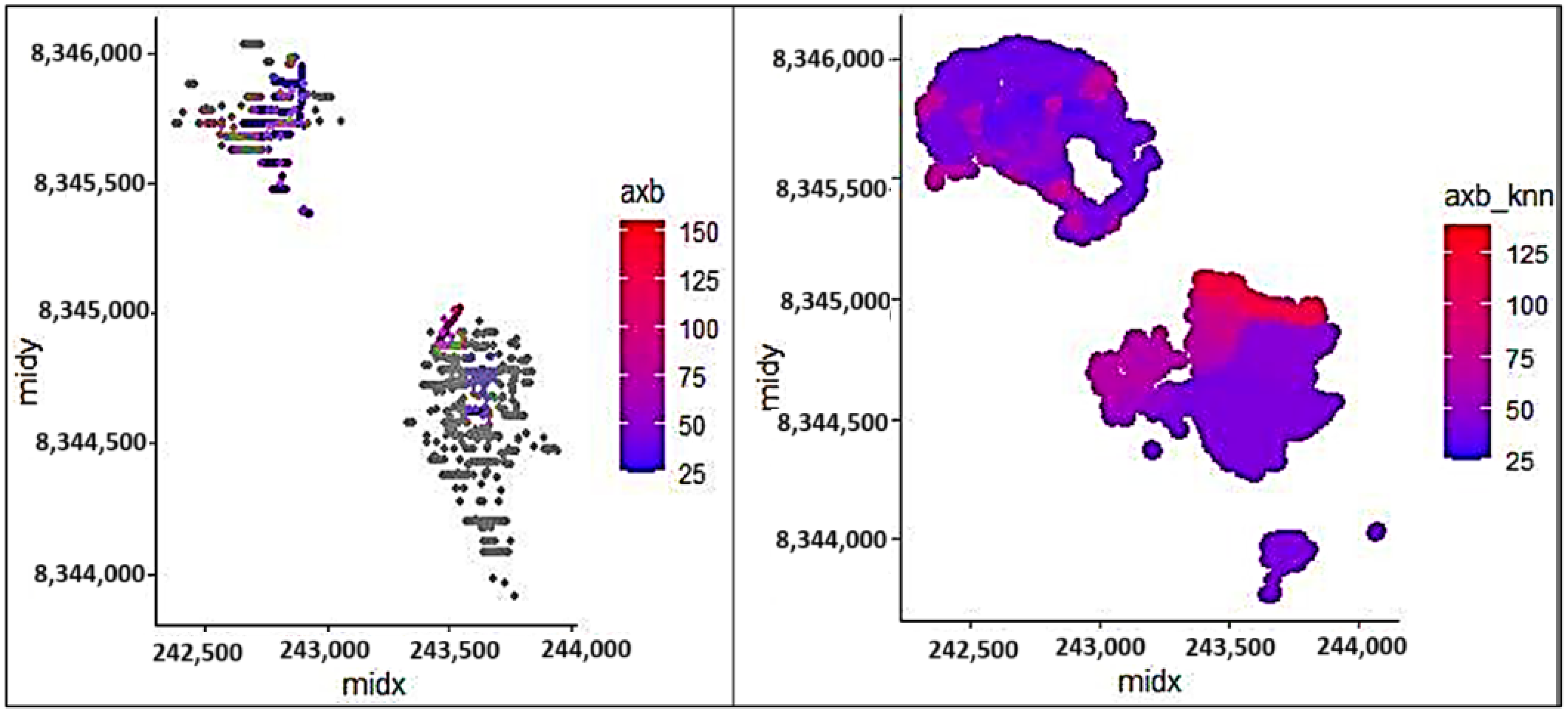
In Figure 4 presents at the left panel shows the spatial distribution of raw A×b sample values collected across the deposit, reflecting the variability in ore breakage characteristics. The right panel presents the modeled A×b distribution generated using the K-Nearest Neighbors (KNN) algorithm, which interpolates values across unsampled areas based on spatial proximity and similarity. This visualization supports the geometallurgical block model by providing a continuous representation of ore hardness, essential for process optimization and mine planning.

2.3. The Bond Ball Work Index Test

Sample requirements: The Bond ball work index laboratory test was created by Bond [53] and uses approx. 7.0 kg of drill core samples, previously crushed 100%-3.350 mm.

Objective: The aim of the test is obtaining a 250 percent circulating load. BWi test results scale-up is achieved using Bond’s third law of comminution [53]:

$$S{E}_{BM}={\displaystyle \frac{P_{MB}\cdot FU{P}_{BM}}{TPH}}=10\cdot BWi\cdot \left({\displaystyle \frac{1}{\sqrt{P_{80}}}}-{\displaystyle \frac{1}{\sqrt{T_{80}}}}\right)$$

(2)

where SE_BM is specific energy consumption, P_BM is nominal power of the mill, FUP_BM is a power use factor, TPH is the plant throughput, BWi is the Bond index, and P₈₀ and T₈₀ are product sizes and feed to the mill, respectively [54]. Recent studies have introduced new approaches to the calculation of the Bond work index for finer samples [55].

In

Table 3. Descriptive Statistics of the BWi Variable.

	BWi
Count	1172
Average	15.1
SD	1.79
Min	8.78
Max	19.1

descriptive statistics of the BWi (Bond Work Index) variable, calculated from 1172 samples. The table presents the mean, standard deviation (SD), and the minimum and maximum observed values. These indicators characterize the variability in ore comminution resistance and are essential for calibrating energy consumption models in grinding circuits.

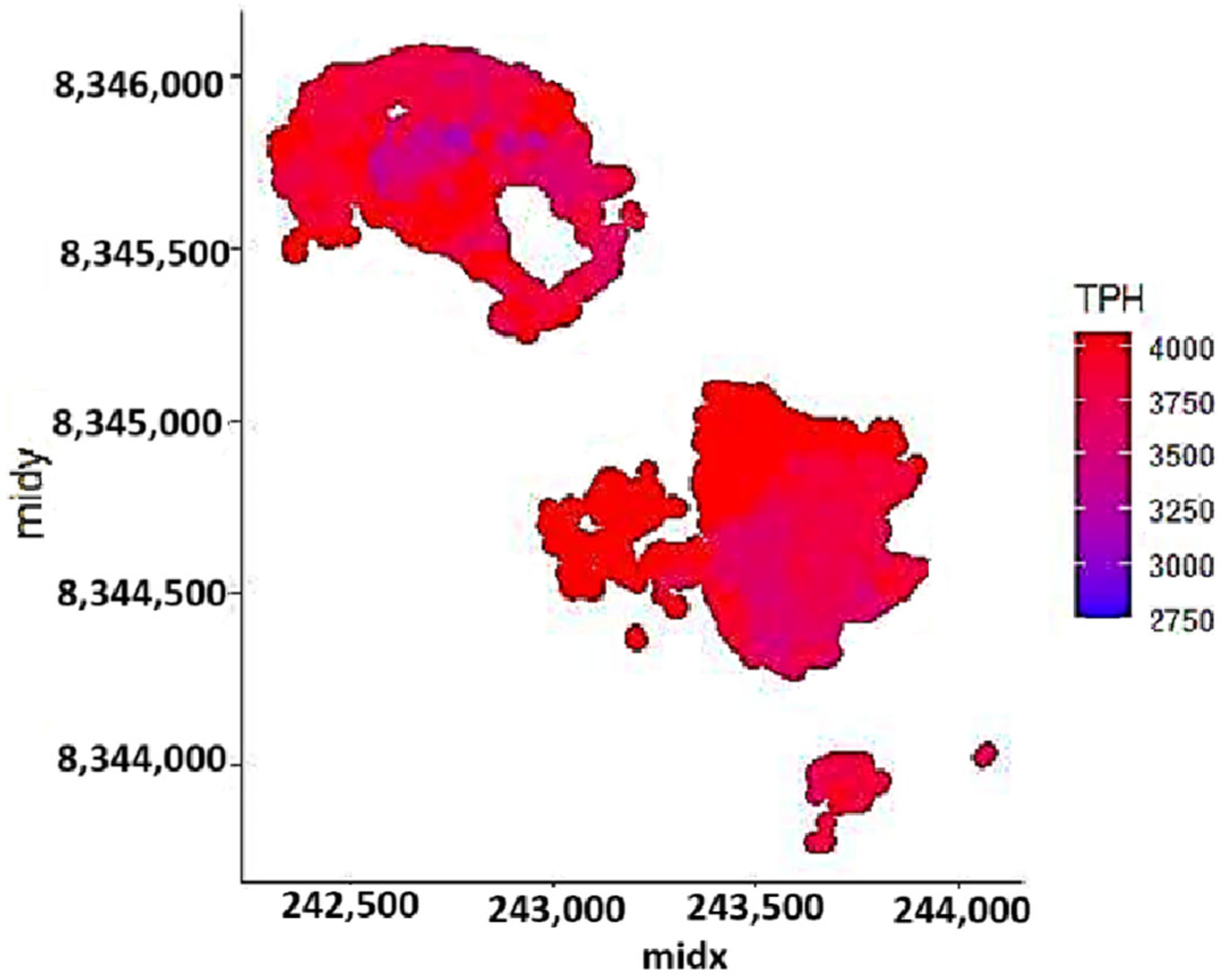
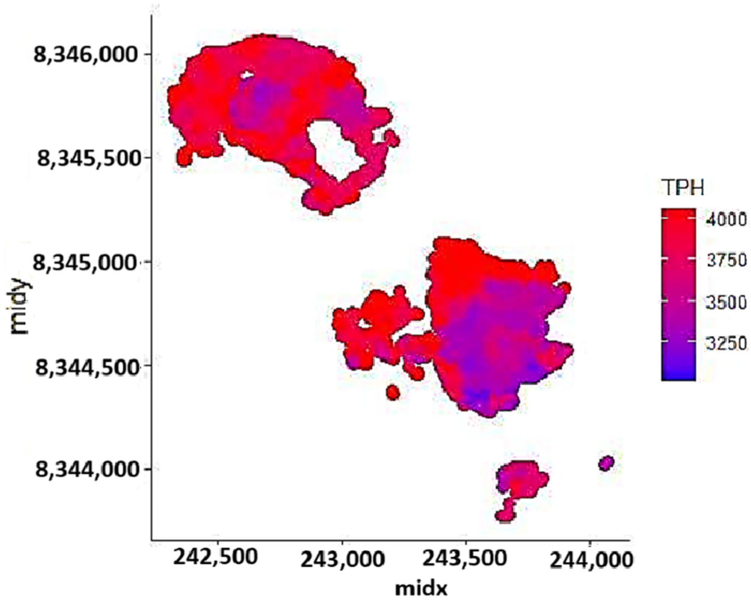
Figure 5 presents the spatial distribution of BWi values based on sample coordinates. The x-axis (“midx”) and y-axis (“midy”) represent spatial midpoints, while the color gradient encodes the variable “witm,” ranging from 9 to 21. The data reveal two prominent clusters, suggesting spatial heterogeneity in BWi values across the study area. This pattern may indicate underlying environmental, biological, or methodological factors influencing the distribution.

2.4. Comminution Indexes Relationships

The Drop Weight Index (DWI, kWh/m³) is directly related to JKDWT test parameters A and b by the following equation [56]:

$$\begin{gathered} DWi=\rho \cdot 96.703\cdot {\left(A\times b\right)}^{-0.992}; \\ {R}^2=0.98 (log.scale) \end{gathered}$$

(3)

where $\rho$ is the mineral density in t/m³.

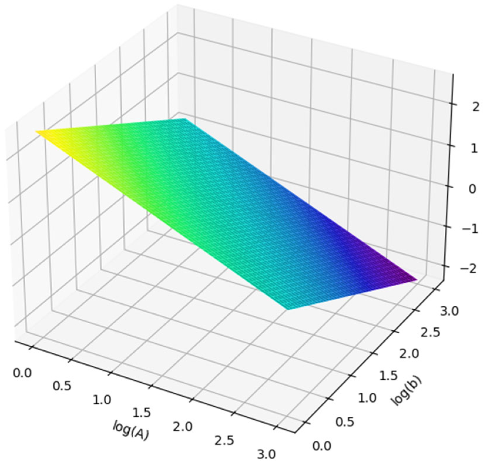
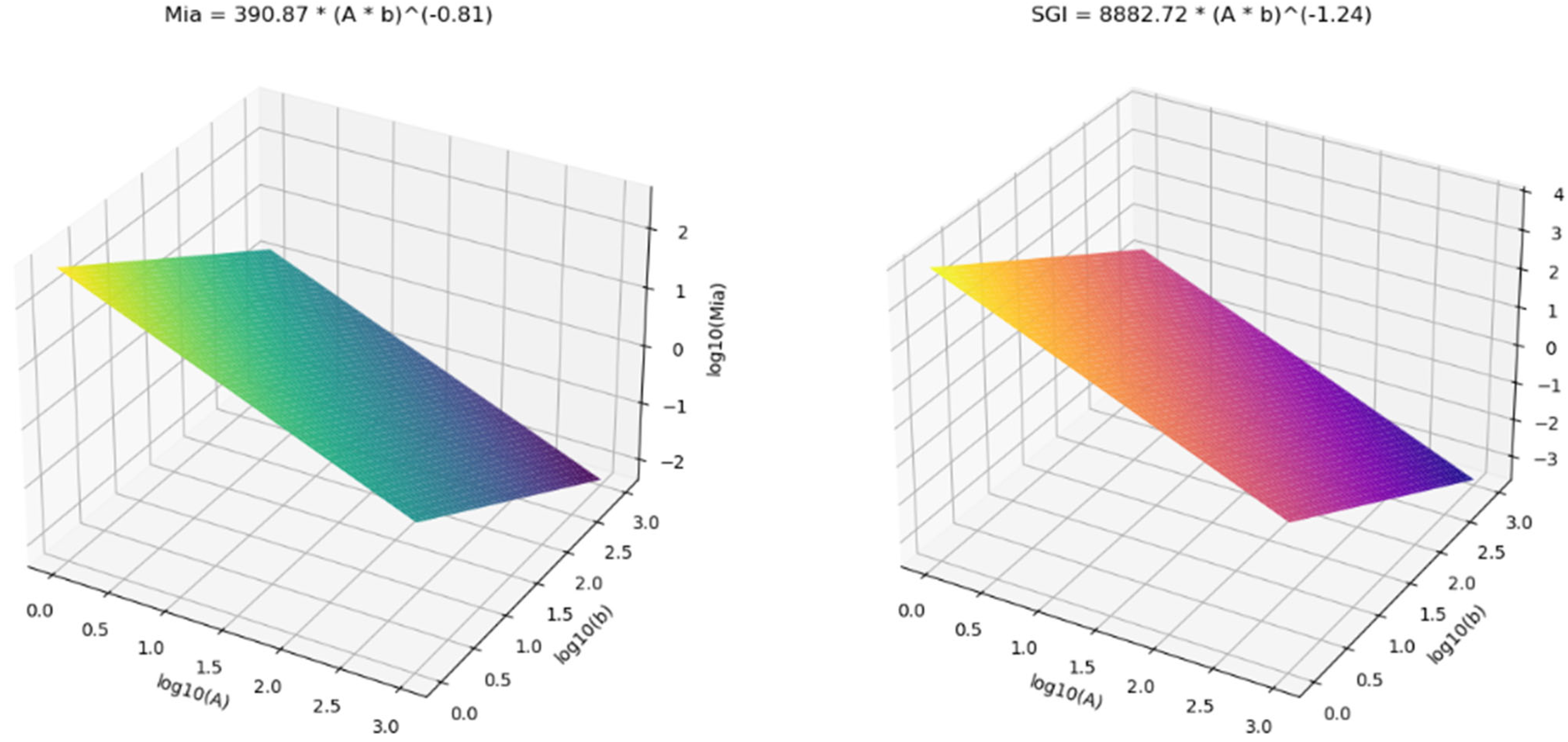
It is possible to relate A×b parameter with the Mia comminution index from the power model developed by Morrell using the following expressions (Figure 6) [57]:

$$\begin{gathered} Mia=390.87\ast {\left(A\times b\right)}^{-0.81}; \\ {R}^2=1.00 (log.scale) \end{gathered}$$

(4)

This reflects a perfectly linear relationship on a log–log scale, as indicated by R² = 1.00.

Mia corresponds to the coarse ore grinding capacity (over 750 microns) in kWh/t.

Finally, the BWi variable is related to Mib of the Morrell [58] power model, as follows (Figure 7):

$$Mib={\displaystyle \frac{18.18}{P_1^{0.295}\ast Gbp\ast \left(p_{80}^{f\left(p_{80}\right)}-f_{80}^{f\left(f_{80}\right)}\right)}}$$

(5)

Mib is the fine ore work index (under 750 microns) (kWh/t), P1 is the test control mesh (microns), Gbp is the net grams of undersize ore per mill revolution (grams/revolution), P₈₀ y F₈₀ correspond to the 80% through size of the product and feed (microns) [49]. The f(P₈₀) and f(F₈₀) are negative exponents that depend on the particle size of the product and the feed, respectively. This functional form allows the model to more accurately capture how grinding efficiency changes with particle size, compared to using a constant exponent.

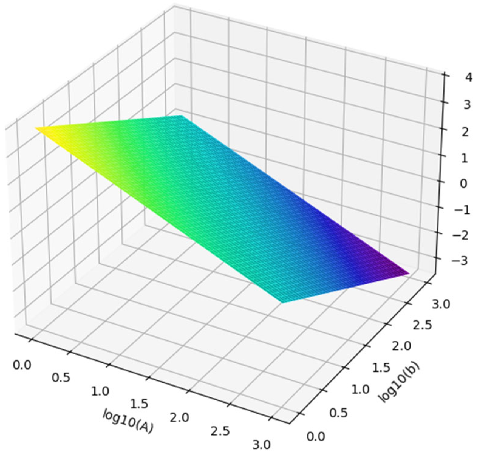
Another comminution test used in industry is the SPI^® or SGI. The kinetic test is run with 2 kg of ore and the time (in minutes) it takes to grind a sample from 80%-12.5 mm to 80%-1.7 mm is measured. The A×b parameter is correlated with the SGI as follows (Figure 8) [58]:

$$\begin{gathered} SGI=8882.72\cdot {\left(A\times b\right)}^{-1.24}; \\ {R}^2=0.83 (log.scale) \end{gathered}$$

(6)

Although the fit is not perfect (R² = 0.83), the relationship remains fairly strong on a log–log scale.

In Figure 9 present at the interpretation:

• Both functions follow a power–law relationship, but SGI decreases more rapidly than Mia with respect to the A×b product.
• This may reflect differences in the nature of the phenomena they represent, particularly if they are related to physical, biological, or economic processes [59].

Graph Analysis:

Wills and Napier-Munn have extensively discussed the principles and techniques of comminution in their work, which provides a foundational understanding for the methodologies applied in this study [60].

2.5. Model Based on DWI and BWi

The specific energy consumption in SAG grinding is defined by the following expression [51]:

$$S{E}_{SAG}=\beta \cdot F_{80}^a\cdot DW{i}^b\cdot {\varphi }^e$$

(7)

where SE_SAG is SAG specific energy consumption, F₈₀ is the 80% through-feed, DWI is the comminution resistance index, ϕ is the critical speed percentage and (β, a, b, e) are constants [61].

The constants β, a, b, and e are calibrated using real plant data or pilot-scale test results.

• β (Beta): A global scaling coefficient
  Adjusts the overall magnitude of energy consumption.
  Its value depends on mill configuration, ore type, and general operating conditions.
  It is tuned to ensure the model predicts realistic specific energy consumption (SE_SAG) values in kWh/t.
• a: Feed size exponent (F₈₀)
  Reflects the influence of feed particle size on energy demand.
  Typical values range from 0.2 to 0.5.
  A positive value indicates that larger feed sizes require more energy.
• b: Drop Weight Index (DWI) exponent
  Captures how sensitive energy consumption is to ore hardness.
  The DWI quantifies resistance to impact breakage.
  Typical values range from 0.5 to 1.0.
  A higher b value means the model is more responsive to hardness variations.
• e: Critical speed exponent (ϕ)
  Describes how mill speed affects energy usage.
  Critical speed is the point at which grinding media begin to centrifuge.
  Typical values range from 0.5 to 1.5, depending on mill design and efficiency.

Parameter Estimation Methods:

• Nonlinear regression using historical plant data.
• Least-squares fitting based on comminution test results.
• Simulation and cross-validation with grinding circuit models [62]

The parameters in Equation (7) are tuned using information from the process, with comminution stage operating in a steady-state regime. On the other hand, BWi results are transformed to specific energy consumption using Equation (2). Since the throughput is the same between SAG and ball grinding stage, the following equality must be fulfilled [26]:

$${\displaystyle \frac{P_{SAG}\cdot FU{P}_{SAG}}{S{E}_{SAG}}}={\displaystyle \frac{P_{BM}\cdot FU{P}_{BM}}{S{E}_{BM}}}$$

(8)

where P_i corresponds to the installed power in the SAG/Balls stage; FUP_i is the fraction of installed power used in size reduction.

The model is solved using Equation (7) to estimate plant TPH; subsequently, a P₈₀ value is imposed, and it is possible to calculate the SAG-ball grinding transfer size using Equations (2) and (8).

2.6. Calculation Workflow for the SAG + Ball Mill Model

Modeling energy consumption in a SAG + ball mill circuit involves a structured sequence of steps, each grounded in empirical data and validated through simulation and plant-scale observations [63,64].

• Step 1: Define Input Parameters

The model begins by specifying key variables:

• F₈₀: Feed particle size to the SAG mill (µm),
• DWI: Drop Weight Index, representing ore hardness (kWh/m³),
• ϕ: SAG mill speed as a percentage of critical speed (%),
• β, a, b, e: Empirical constants that scale and shape the energy model,
• P_SAG, P_BM: Installed power for SAG and ball mills (kW),
• FUP_SAG, FUP_BM: Fraction of power utilized in each stage,
• SE_BM: Specific energy for ball milling, typically derived from the Bond Work Index (BWi), and
• P₈₀: Target product size (µm).

These parameters are essential for simulating energy demand and throughput under varying operational conditions [63,65].

• Step 2: Calculate Specific Energy Consumption in SAG

The specific energy consumed in the SAG grinding is estimated using a power–law expression:

$$S{E}_{SAG}=\beta \cdot F_{80}^a\cdot DW{i}^b\cdot {\varphi }^e$$

This formulation captures the nonlinear influence of feed size, ore hardness, and mill speed on energy usage [63,64].

• Step 3: Estimate Plant Throughput

Throughput (TPH) is calculated by dividing the effective power input by the specific energy:

$$TPH={\displaystyle \frac{P_{SAG}\cdot FU{P}_{SAG}}{S{E}_{SAG}}}$$

This step links energy efficiency to production capacity, enabling performance benchmarking [65].

• Step 4: Apply Energy Balance Between Stages

An energy balance is applied to ensure consistency between the SAG and ball mill stages:

$${\displaystyle \frac{P_{SAG}\cdot FU{P}_{SAG}}{S{E}_{SAG}}}={\displaystyle \frac{P_{BM}\cdot FU{P}_{BM}}{S{E}_{BM}}}$$

This balance can be used to validate or adjust the ball mill energy estimate or the transfer size between stages [64].

• Step 5: Determine Transfer Size (T_t)

Using the ball mill energy equation (e.g., based on BWi), the transfer size between SAG and ball milling can be back-calculated to satisfy the energy balance.

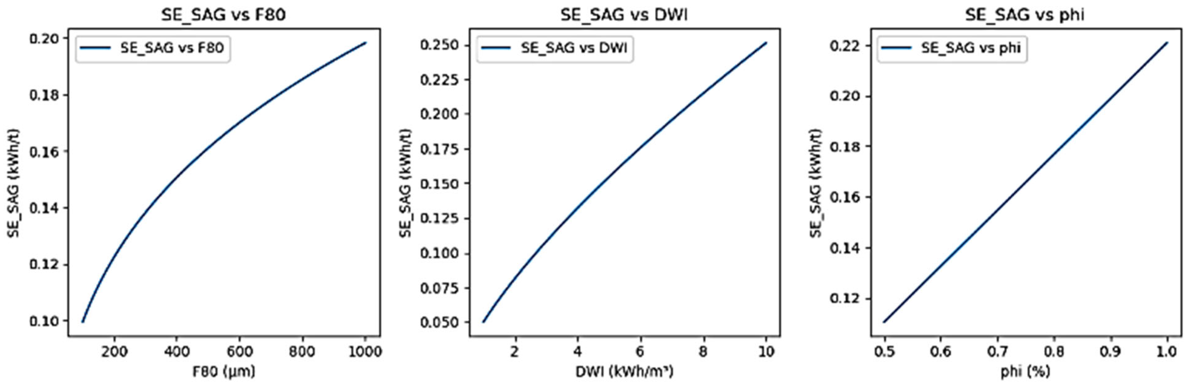
The specific energy consumption in SAG grinding (SE_SAG) is analyzed by individually modifying each of the model’s key parameters, as illustrated in Figure 10.

2.7. Model Based on SMC (Mia, Mib) and BWi

The following equation is defined for specific energy consumption per grinding stage [29]:

$$\begin{gathered} f\left({\mathrm{F}}_{80}\right)=-\left(0.295+{\mathrm{F}}_{80}\cdot {10}^{-6}\right) \\ f\left({\mathrm{P}}_{80}\right)=-\left(0.295+{\mathrm{P}}_{80}\cdot {10}^{-6}\right) \\ W\left(M_i,{\mathrm{F}}_{80},{\mathrm{P}}_{80}\right)=M_i\cdot 4\cdot \left({\mathrm{P}}_{80}^{f\left(P_{80}\right)}-{\mathrm{F}}_{80}^{f\left(F_{80}\right)}\right) \end{gathered}$$

(9)

where F₈₀ is the 80% feed through size, P₈₀ is the 80% product through size, M_i is the specific energy index for size reduction, and W is the grinding stage specific energy consumption.

2.8. Interpretation of Key Components in the Energy Model

Understanding the role of each variable in the particle size–energy relationship is essential for accurate modeling of comminution processes [63].

• F₈₀ and P₈₀

• F₈₀ refers to the particle size below which 80% of the feed material passes, while P₈₀ represents the same threshold for the product stream.
• These metrics are typically expressed in micrometers (µm) or millimeters (mm), depending on the scale of the operation [64].
• They are fundamental in defining the energy required for size reduction, as used in classical and modified comminution models [65].

• f(F₈₀) and f(P₈₀)

• These are variable exponents that adjust based on particle size.
• As F₈₀ or P₈₀ increase, the corresponding exponent becomes more negative, reducing the overall energy contribution of that term.
• This approach allows for a more flexible and realistic representation of energy behavior compared to fixed-exponent models [66].

• M_i (Specific Energy Index)

• M_i represents the specific energy required to reduce one tonne of material to a target size, expressed in kWh/t.
• It is also known as the work index or the comminution index and varies depending on the ore type and grinding mechanism (e.g., Mia for impact, Mih for high-pressure grinding, Mic for crushing) [63].
• This parameter is critical for comparing ore hardness, designing grinding circuits, and calibrating simulation models [66].

• W (Specific Energy Consumption)

• W quantifies the energy consumed per tonne of material processed, typically in kWh/t.
• It is calculated using a modified energy equation that incorporates M_i, particle size terms, and a scaling factor (commonly 4).
• The interpretation of W depends on the context:
• If M_i corresponds to a SAG-related index (e.g., DWi or Mia), then W reflects energy use in the SAG stage.
• If M_i is the Bond Work Index (BWi), then W represents energy in the ball grinding stage [67].
• In geometallurgical models, different M_i values are used for each stage (e.g., Mib, Mih, Mia, and Mic) to reflect stage-specific energy behavior [68].

This formulation is a generalized version of the particle size–energy equation, similar to Bond’s law but with variable exponents. It estimates the energy required to reduce particle size during grinding, offering more flexibility and accuracy in modeling complex ore behaviors [66].

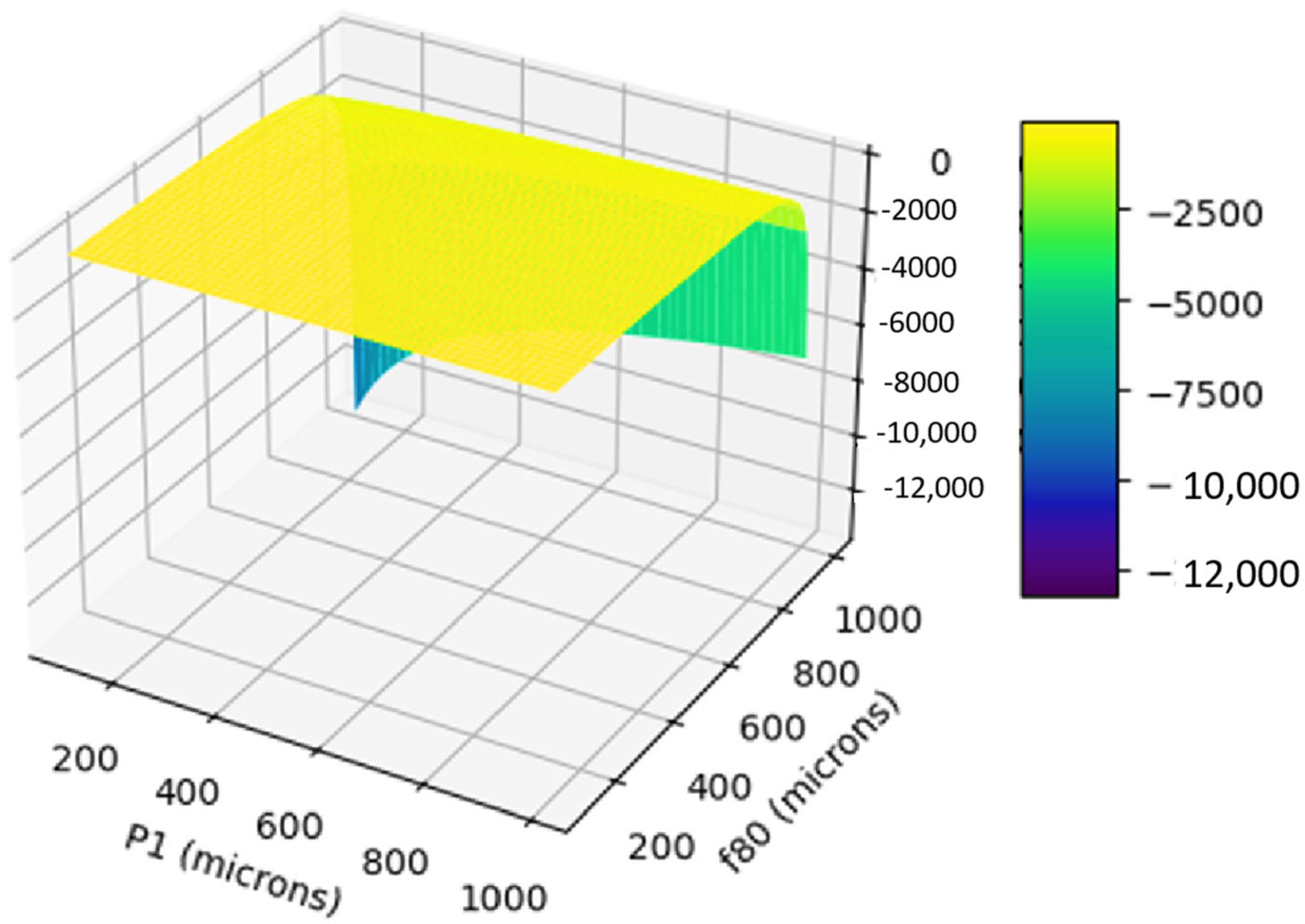
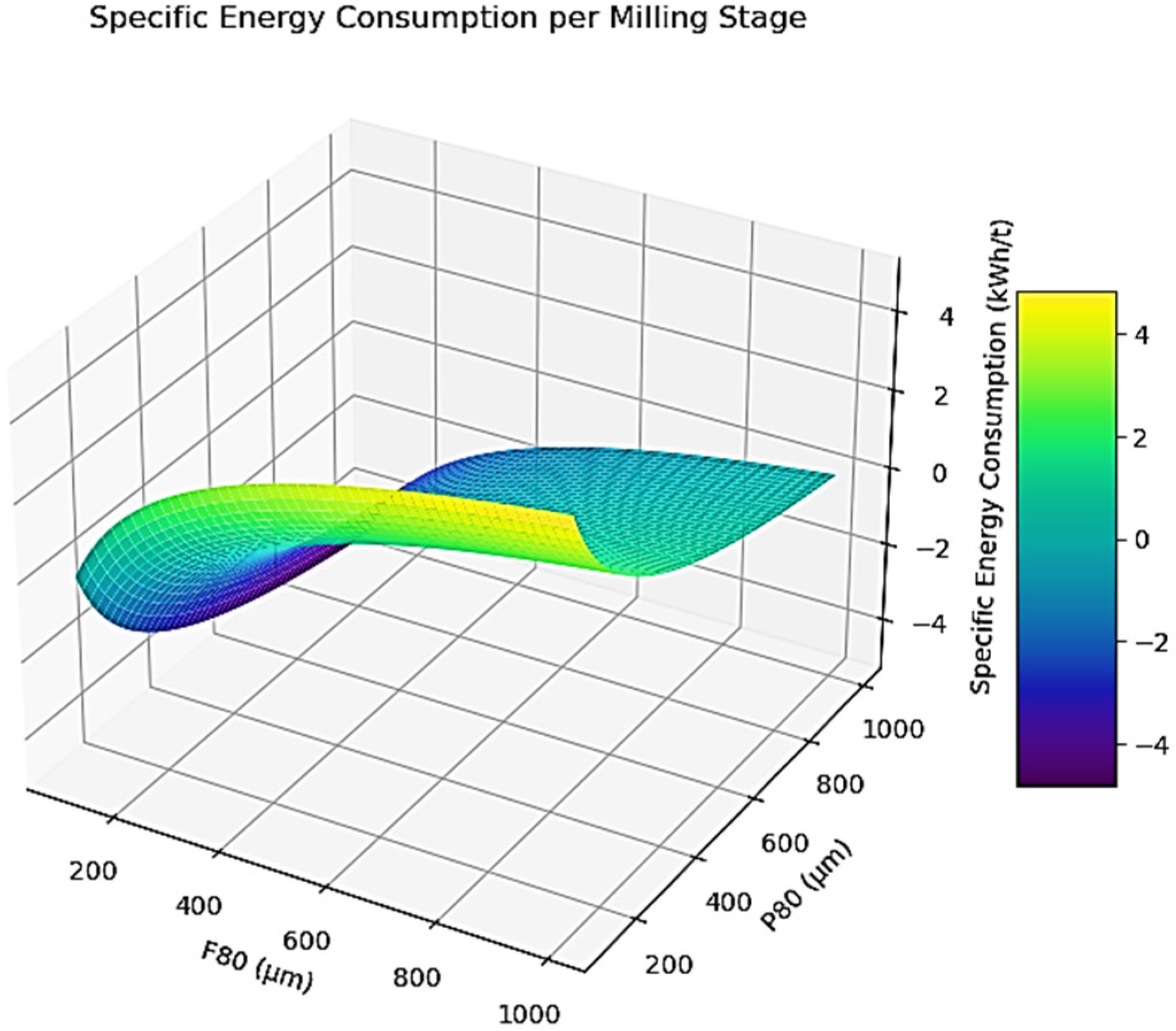
We can generate a 3D plot (Figure 11) showing how W varies with F₈₀ and P₈₀, assuming a typical M_i value (e.g., 10 kWh/t). This would help illustrate how energy demand increases with greater size reduction and how the curvature of the surface reflects the nonlinear nature of the model.

Some observations are:

• A greater difference between F₈₀ and P₈₀ leads to higher energy consumption, as expected.
• When F₈₀ ≈ P₈₀, the energy required approaches zero, indicating minimal or no size reduction.
• The curved surface reflects the nonlinear relationship introduced by the square root terms in the energy equation.

The SAG grinding stage specific energy consumption is determined as [69]:

$$S{E}_{SAG}=K_1\cdot W\left(Mia,{\mathrm{F}}_{80},T_{80}\right)$$

(10)

where SE_SAG corresponds to the SAG grinding specific energy consumption, Mia is the energy index related to size reduction in coarse particles (>750 microns), and K₁ = 0.95 for the SAG mill operating with crushed pebbles.

The ball grinding stage specific consumption is determined as:

$$\begin{gathered} {SE}_{coarse}=K_1\cdot W(Mia,T_{80},750) \\ {SE}_{fine}=W\left(Mib,750,{\mathrm{P}}_{80}\right) \\ {SE}_{BM}={SE}_{coarse}+{SE}_{fine} \end{gathered}$$

(11)

where SE_coarse corresponds to the specific energy consumption for grinding particles above 750 microns, SE_fine is the specific energy consumption for grinding particles below 750 microns, SE_BM is the ball grinding stage specific energy consumption, and Mib is the energy index related to particle size reduction below 750 microns. K₁ = 1.00 for the ball mill operating without crushing pebbles [70,71].

Although the same Mia index is used, it is now applied to a sub-stage within ball milling, specifically for the coarse fraction. The value of 750 µm acts as a threshold between coarse and fine particles.

In Equation (11), W (Mia, T₈₀, 750) refers to the energy consumption of the coarse fraction within the ball grinding stage, while W(Mib, 750, P₈₀) covers the fine fraction.

Since the throughput is the same between both systems, the analogous equality like that expressed in Equation (8) must be fulfilled. The model is solved using Newton-Raphson method on Equation (8) evaluated in Equations (10) and (11); the solution converges to a raw value of T₈₀ (restricted by the maximum transfer size). Subsequently, the system TPH is calculated (restricted by the maximum TPH). Finally, P₈₀ value is corrected in cases where the system is restricted by screen opening or transport capacity.

2.9. Model Based on SGI and BWi

SGI or SPI results (SGS commercial lab version) are industrially scaled using the formula [72]:

$${SE}_{SAG}={\displaystyle \frac{P_{SAG}\cdot FU{P}_{SAG}}{TPH}}=K\cdot {\left({\displaystyle \frac{SGI}{\sqrt{T_{80}}}}\right)}^n$$

(12)

where SE_SAG is the specific energy consumption, P_SAG is the mill nominal power, FUP_SAG is a power use factor, TPH is the flow of ore processed, K is a parameter equal to 5.59, n is a parameter equal to 0.55, and T₈₀ is the mill product size [47].

Integration with BWi and Energy Balance

Model Stages:

Transformation of the Bond Work Index (BWi) into specific energy consumption using a Bond-type equation (Equation (2)).

An energy balance is imposed between the SAG and ball mill stages:

The system is solved using the Newton-Raphson method, simultaneously evaluating:

○

Equation (12) (SGI),

○

Equation (2) (BWi), and

○

Equation (8) (Power balance).

○

This approach allows for determining a value of T₈₀ that balances the system.

Model Constraints:

• The value of T₈₀ is limited by the maximum transfer size accepted by the ball mill.
• TPH is also constrained by the plant’s maximum capacity.
• The value of P₈₀ may be adjusted if there are limitations due to:

  ○

  Screen aperture, and

  ○

  Conveyor capacity.

Model Applications:

• Design and simulation of SAG + ball mill grinding circuits.
• Evaluation of expansion scenarios or ore type changes.
• Optimization of specific energy consumption and throughput.

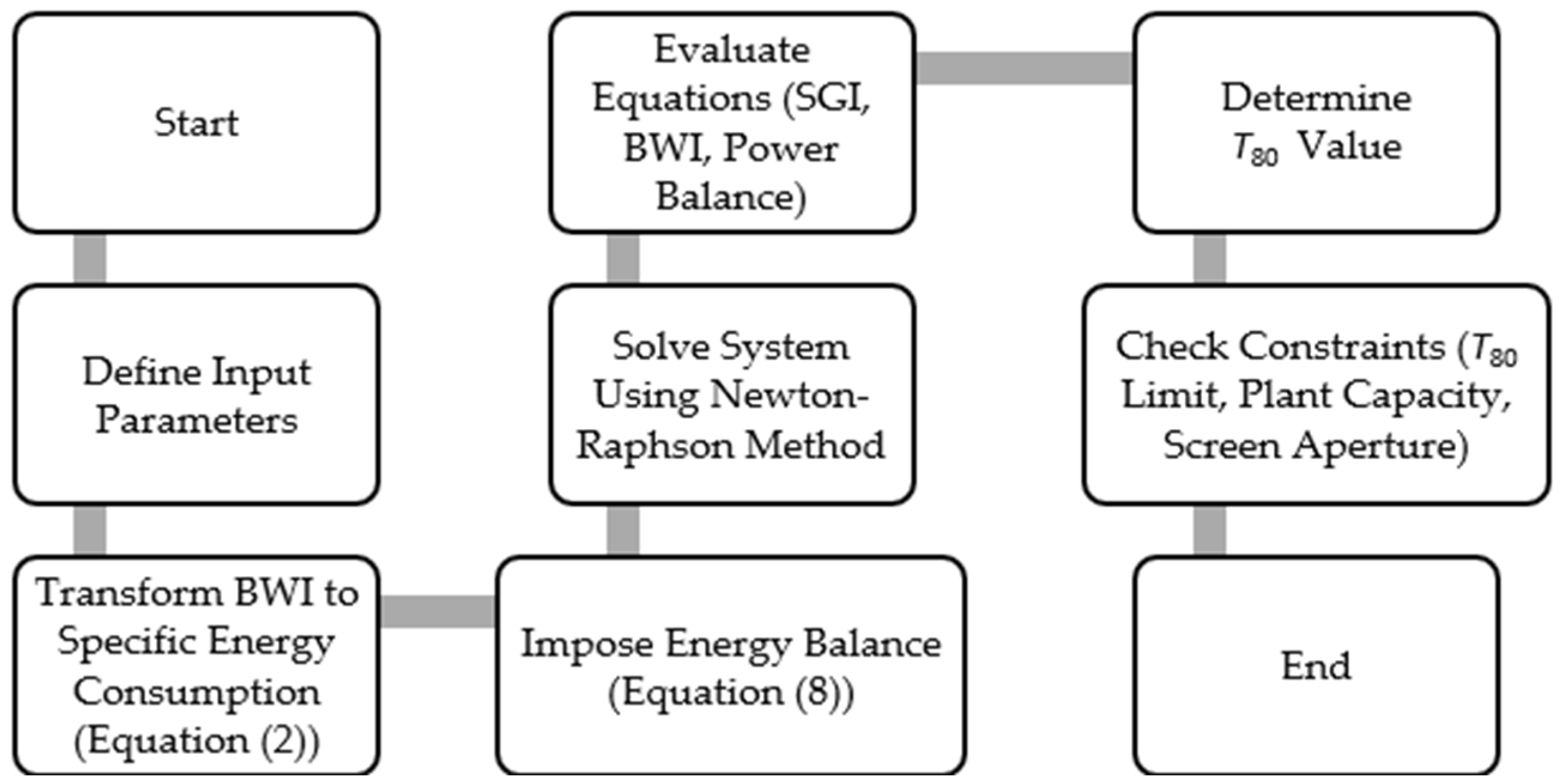
Abstract the key steps of the process, from the transformation of the BWi to the evaluation of operational constraints such as transfer size (T₈₀), plant capacity, and screen aperture (Figure 12):

• Start: The process begins with the objective of integrating the Bond Work Index (BWi) into a SAG + Ball mill energy model, ensuring energy balance across stages.
• Define Input Parameters: This step involves specifying all necessary inputs, including:
  • BWi (Bond Work Index),
  • Installed power for SAG and ball mills,
  • Utilization factors (FUP), and
  • Initial estimates for transfer size (T₈₀), product size (P₈₀), and energy indices (e.g., Mia and Mib).
• Transform BWi to Specific Energy Consumption (Equation (2))
  Using a Bond-type equation, the BWi is converted into specific energy consumption (SE_BM) for the ball mill stage. This allows comparison with the SAG stage energy.
• Impose Energy Balance (Equation (8))
  An energy balance equation is applied to ensure that the energy input and output across the SAG and ball mill stages are consistent:
• Solve System Using Newton-Raphson Method
  The system of nonlinear equations is solved iteratively using the Newton-Raphson method to find a consistent solution for T₈₀ and energy values.
• Evaluate Equations (SGI, BWi, Power Balance)
  At each iteration, the model evaluates:
  • SGI-based energy (Equation (12)),
  • BWi-based energy (Equation (2)), and
  • Power balance (Equation (8)).
  This ensures all components are aligned.
• Determine T₈₀ Value
  Once convergence is achieved, the model outputs the optimal T₈₀ (transfer size) that satisfies the energy balance and system constraints.
• Check Constraints
  The solution is validated against operational limits:
  • Maximum transfer size accepted by the ball mill,
  • Plant throughput capacity (TPH), and
  • Screen aperture and conveyor limitations.
  Adjustments are made if any constraint is violated.
• End
  The process concludes with a validated and balanced energy model, ready for use in circuit design, simulation, or optimization.

On the other hand, the BWi results are transformed to specific energy consumption using Equation (2). Finally, since the throughput is the same between both systems, the analogous equality like that expressed in Equation (8) must be fulfilled. The model is solved using the Newton-Raphson method on Equation (8) evaluated in Equations (2) and (12); the solution converges to a raw value of T₈₀ (restricted by the maximum transfer size) [72]. Subsequently, the TPH of the system is calculated (restricted by the maximum TPH). Finally, P₈₀ value is corrected in cases where the system is restricted by screen opening or transport capacity [72,73].

Process restrictions

From a practical point of view, there is a maximum throughput (TPH_max) usually determined by transport considerations in the system. Additionally, materials with a particle size larger than the screen opening mesh will remain in the SAG stage; therefore, there is a maximum transfer size (T_80max). The above conditions impose limits on the throughput provided by Equations (10) and (12).

The maximum T₈₀ represents the coarsest particle size that can be effectively transferred from the SAG mill to the ball mill without compromising grinding efficiency or overloading the downstream equipment. This limit is typically defined by:

• The ball mill’s feed size capacity, which is influenced by liner design, ball size, and mill diameter.
• The hydraulic transport capacity of the system, including conveyors and pumps, must handle the coarse fraction without blockages or excessive wear [73].

TPH Limit—Plant Throughput

The maximum TPH (tons per hour) is constrained by:

• The installed power and utilization efficiency of the grinding mills.
• The classification system (e.g., hydrocyclones or screens), which must maintain separation efficiency at high flow rates.
• The ore characteristics, such as hardness and density, which affect the residence time and energy demand [74,75].

Hydraulic Limit as Governing Factor

In both cases, the hydraulic limit—the ability of the system to transport and classify slurry efficiently—acts as the governing constraint. If exceeded, it can lead to:

• Reduced grinding efficiency
• Increased circulating loads,
• Premature wear of equipment, and
• Risk of system instability or shutdown [76].

Application in Predictive Models

These maximum values are used as boundary conditions in simulation tools and geometallurgical models to:

• Prevent unrealistic predictions of throughput,
• Ensure safe and efficient operation under varying ore types, and
• Support decision making in circuit design and expansion planning.

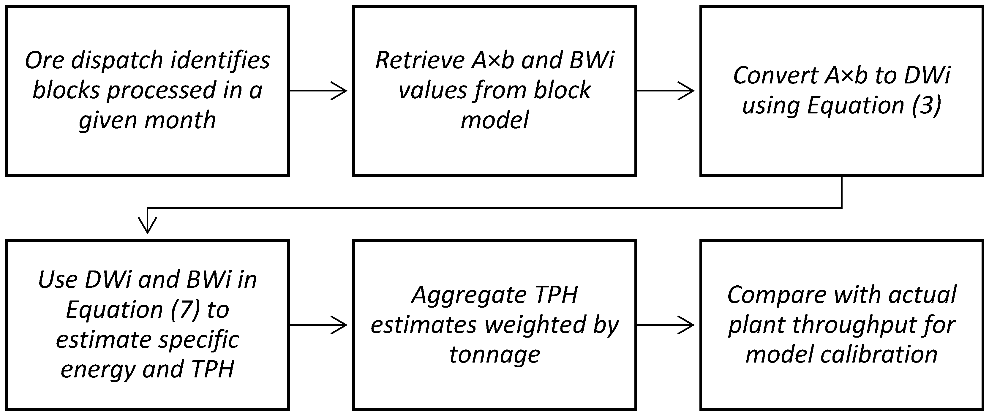
Figure 13 illustrates the operational constraints defined by hydraulic and screen opening limits in relation to throughput (TPH) and Mia. The vertical axis represents the throughput in tons per hour (TPH), while the horizontal axis corresponds to Mia, a parameter likely related to ore hardness or the energy index. The bold black line delineates two distinct operational boundaries: a horizontal segment indicating the Hydraulic Limit, and a descending curve representing the Screen Opening Limit. These boundaries define the feasible operating region for the system, highlighting the trade-offs between material throughput and mechanical constraints.

3. Results

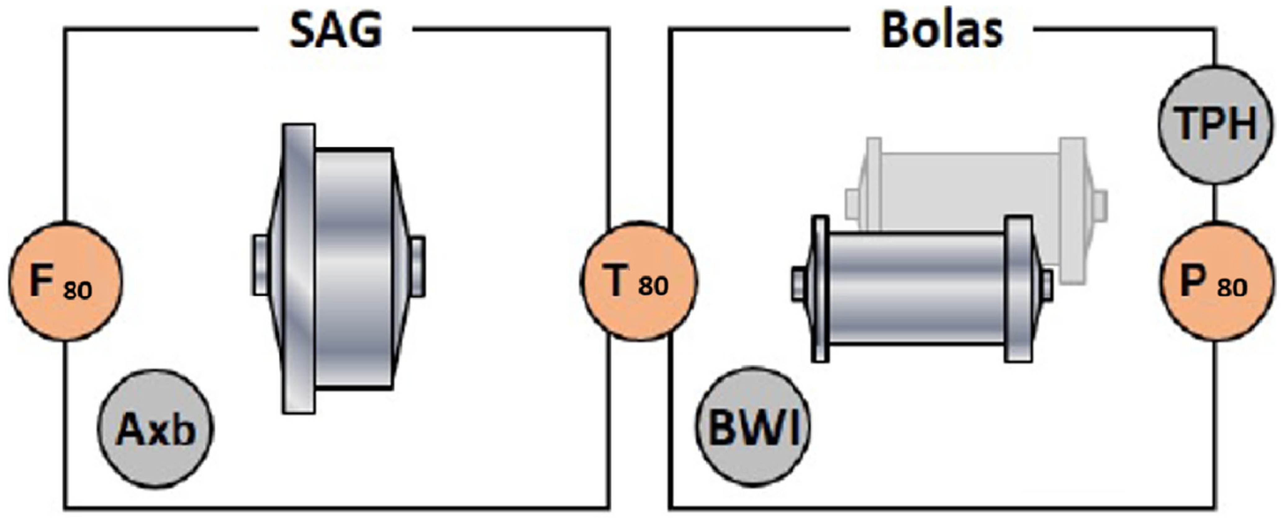
The processing capacity model was conceptualized into two components: the SAG grinding stage and the ball grinding stage. This diagram illustrates (Figure 14) the key parameters involved in the comminution process within a typical SAG (semi-autogenous grinding) and Ball Mill circuit. In the SAG section, the feed characteristics are defined by F₈₀ (the 80% passing size of the feed) and A×b (a parameter from the JK Drop Weight Test indicating ore hardness). The Ball Mill section includes operational and product parameters such as TPH (tons per hour), P₈₀ (the 80% passing size of the product), and BWi (Bond Work Index). The intermediate parameter T₈₀ represents the transfer size between the two grinding stages. This schematic is useful for understanding the relationships between ore characteristics, mill throughput, and energy requirements in mineral processing circuits.

The performance models were implemented using the open-source software R/RStudio [77,78]. Additionally, the correctness of the code was verified by independently implementing the models in Microsoft^® Excel^® 2021 and Microsoft^® Visual Basic^® 2021 for Applications. Geometallurgical modeling was applied for performance estimation [79,80,81].

The workflow for the three evaluated processing models is summarized in the following Figure 15:

The workflow activities include

• Library loading: Required R libraries are loaded for code execution.
• Function loading: Specific functions used in the modeling process are enabled.
• Data loading: The following data files are read:

  ○

  PI-System data file containing comminution circuit variables.

  ○

  Database with results from JK Drop Weight Test (JKDWT) samples.

  ○

  Database with the Bond Work Index (BWi) test results.

  ○

  Block model identifying mined blocks processed during the evaluation period.

• Data cleaning: Quality control and necessary modifications are applied to raw data for use in the modeling process.
• A×b calculation: Due to low sample density in this area, it must be verified whether estimations exist; otherwise, the block model must be populated.
• Application of the processing model to mined blocks: The processed flow calculation algorithm is applied to the mined blocks from 1 January 2018, to 1 November 2020.
• Results verification: General consistency of the results is verified at the block model level.
• Block model volumetrics: Volumetric calculations are performed to determine TPH, T₈₀, and P₈₀ values monthly.
• Reconciliation: Plant and modeled results for TPH, T₈₀, and P₈₀ are compared monthly.
  The model parameters were determined using plant data collected over a 36-month period (PI system). Specifically, the following variables and process specifications were considered:

  ○

  Power usage fraction for SAG and ball milling.

  ○

  Total installed power for SAG and ball milling (kW).

  ○

  Feed size at 80% passing for SAG (microns).

  ○

  Final product size at 80% passing (microns).

  ○

  Maximum transfer size from SAG to ball milling (microns).

  ○

  Maximum system throughput (t/h).

  ○

  Critical speed of the SAG mill.

  To ensure steady-state operation, only months with at least 80% of the time operating at 95% or more were considered.

• Historical or expected average values:
• SAG feed size (F₈₀): 71,273.25 microns,
• Ball mill product size (P₈₀): 229.13 microns,
• SAG power usage (FUP_SAG): 21,507 kW,
• Ball mill power usage (FU_PBM): MB1 = 15,150 kW, MB2 = 14,934 kW,
• Installed SAG power (P_SAG): 24,000 kW,
• Installed ball mill power (P_BM): 32,800 kW,
• Maximum system throughput (TPHmax): 4058 t/h, and
• Maximum transfer size from SAG to ball milling (T₈₀max): 19,783 microns.
• Block model estimates include

  ○

  A×b, for Mia calculation;

  ○

  BWi, grams per revolution (Gbp), feed and product sizes (F₈₀, P₈₀), and control mesh P1, for Mib calculation [46];

  ○

  Note: If complete BWi data is unavailable, Mib is estimated using a linear relationship: Mib = a × BWi + b.

Given a target P₈₀, the algorithm estimates T₈₀ and TPH. In specific cases, P₈₀ is recalculated to satisfy the system of equations under boundary conditions.

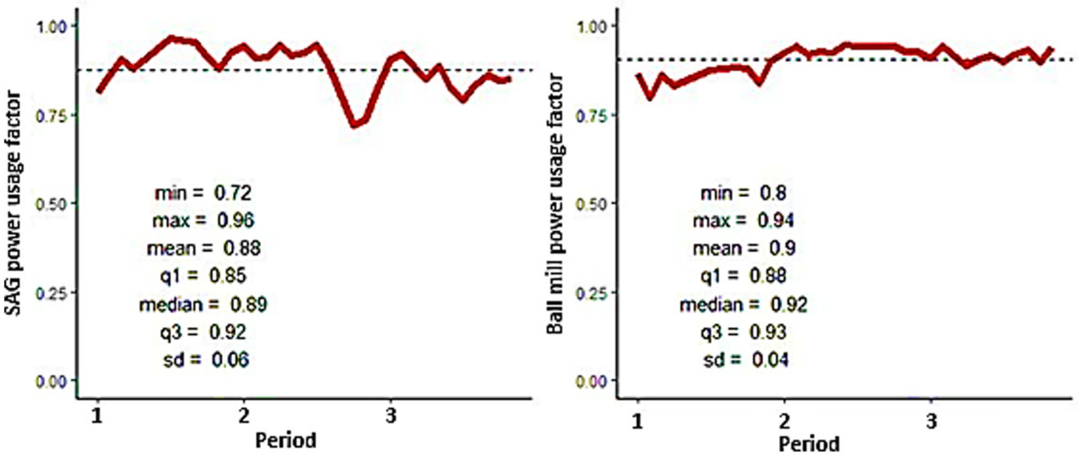
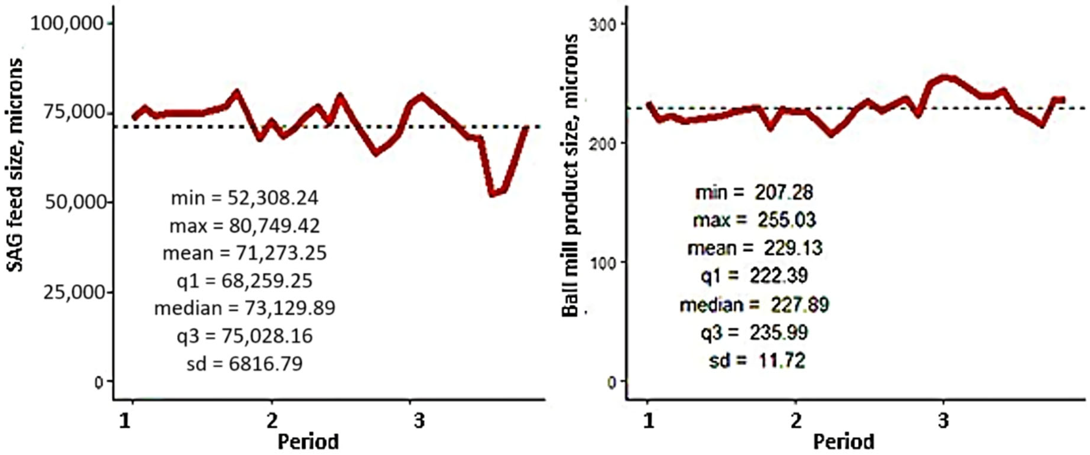
The following figures (Figure 16, Figure 17 and Figure 18) present time series and descriptive statistics for six key variables relevant to the modeling and reconciliation process. The dotted line in each graph represents the average value of the variable over the period considered.

The DWi-BWi Model: The DWi-BWi model was evaluated using baseline values for critical parameters. Sensitivity analysis revealed that the model did not respond well to parameter adjustments, often resulting in maximum throughput values. The spatial distribution of TPH estimated by the block model is shown in Figure 19.

The Morrell Power Model: The Morrell power model was also evaluated using baseline values for critical parameters. The model exhibited variability in TPH values across different pits, with Pit 1 showing the highest variability. Nonetheless, the model provided reasonable predictions for both processed tonnage and product size. The spatial distribution of TPH is presented in Figure 20.

The SGI-BWi Model: The SGI-BWi model was evaluated under similar conditions. It demonstrated comparable variability across pits and yielded reasonable predictions for processed tonnage and product size. The spatial distribution of TPH is also shown in Figure 21.

Model Reconciliation and Predictive Accuracy

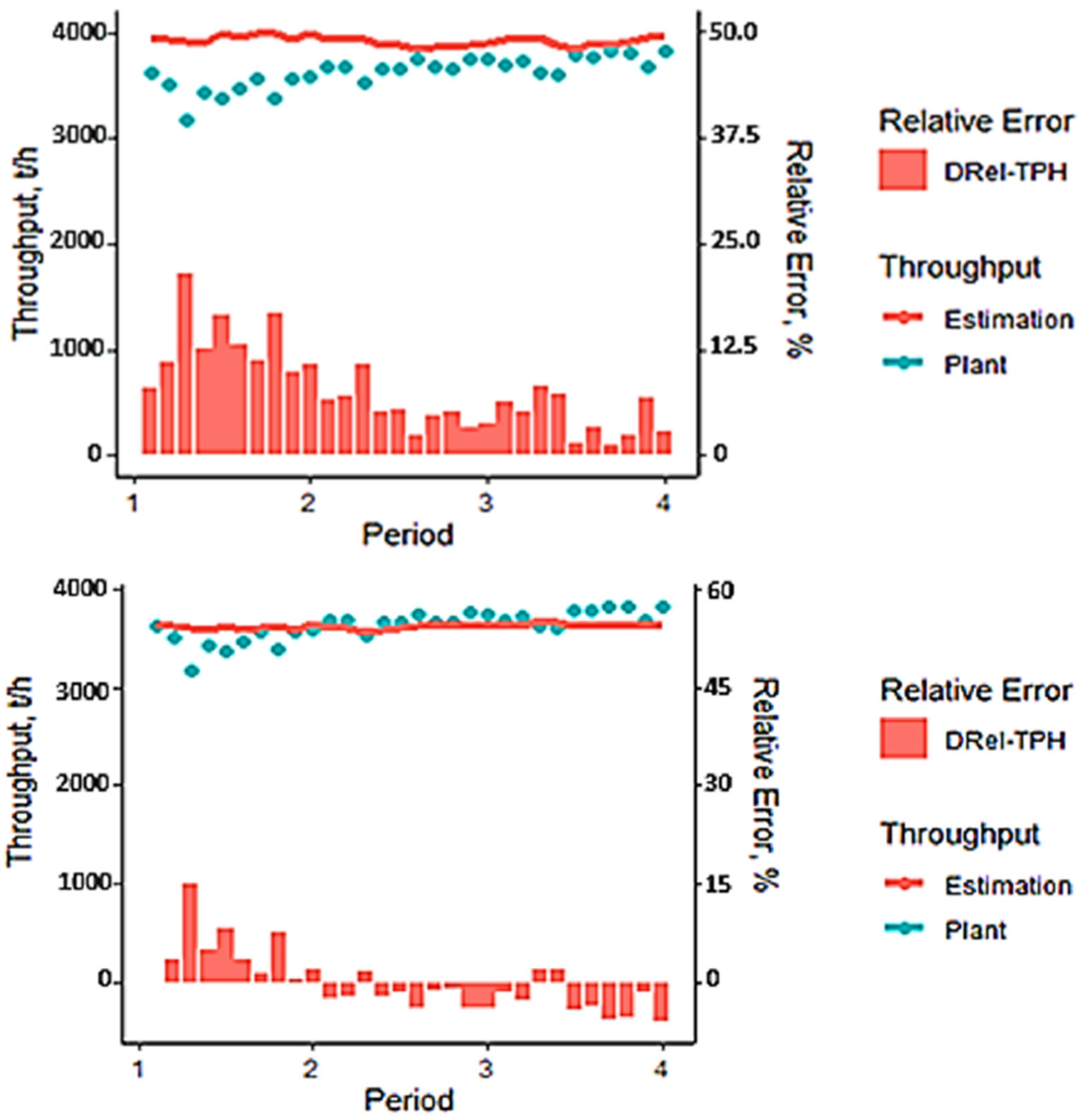
DWi-BWi Model Reconciliation

The reconciliation between plant performance and the DWi-BWi model output is shown below.

In this analysis, the predictive capability of the parametric model defined by Equation (7) was evaluated. The fundamental parameters (β, a, b, e) were initially calibrated using operational plant data. However, the results from this preliminary calibration stage revealed limited predictive accuracy, as illustrated in Figure 22 (top panel), where significant dispersion is observed between estimated values and actual plant data, along with high relative errors.

To address this, a block-wise optimization strategy was implemented, aimed at minimizing the fitting error through iterative reconfiguration of the model parameters. This methodology led to a substantial improvement in estimation accuracy, as shown in Figure 22 (bottom panel), where a notable reduction in relative error magnitude and greater alignment between estimated and actual curves is evident.

Quantitatively, the first model iteration (without optimization) yielded a root mean square error (RMSE) of 351 tons per hour (t/h), indicating a considerable deviation from actual system behavior. After applying the optimization algorithm, the RMSE was reduced to 147 t/h, representing a significant improvement in model fit.

However, while parameter optimization can enhance short-term model accuracy, it introduces inherent risks of overfitting. Excessive adaptation to historical data may compromise the model’s generalization capacity and predictive robustness in future scenarios—particularly in long-term planning under the Life of Mine (LOM) framework. Therefore, caution is advised when applying intensive optimization techniques, favoring models that balance fit quality with generalization capability.

SMC (Mia, Mib)—BWi Model Reconciliation

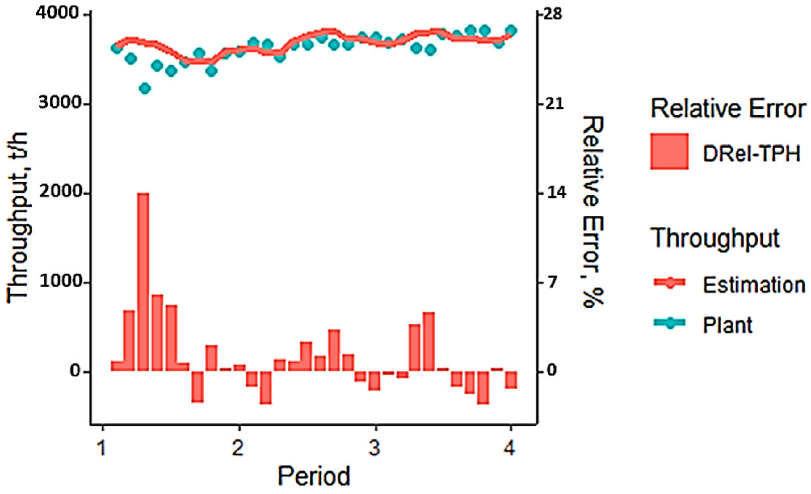
Figure 23 presents a comparative analysis between actual plant throughput and estimates generated by the hybrid model based on the comminution parameters Mia and Mib, integrated with the Bond Work Index (BWi). This reconciliation assesses the model’s ability to replicate the dynamic behavior of throughput (t/h) across different operational periods.

The chart uses overlaid bars to compare estimated and actual throughput values, while the solid line represents the relative error percentage (DRel-TPH) for each period. This dual representation facilitates the identification of discrepancies and quantifies the model’s predictive accuracy.

Except for the first period, where a more pronounced deviation is observed, the model captures the observed throughput trend with reasonable fidelity. In subsequent periods, the difference between estimated and actual values remains within acceptable margins, suggesting proper calibration under stable or recurring operational conditions.

From a quantitative standpoint, the model based on the SMC methodology (incorporating Mia and Mib) and BWi achieves an RMSE of 143 t/h. This indicates a high level of accuracy, especially considering the inherent variability of comminution processes and the complexity of interactions among ore properties, operating conditions, and circuit configuration.

Nevertheless, the model’s validity should be assessed not only by its historical fit but also by its predictive robustness in future scenarios. Its consistency across multiple periods and low RMSE position it as a valuable tool for operational planning and strategic decision making in medium- and long-term mining contexts.

SGI-BWi Model Reconciliation

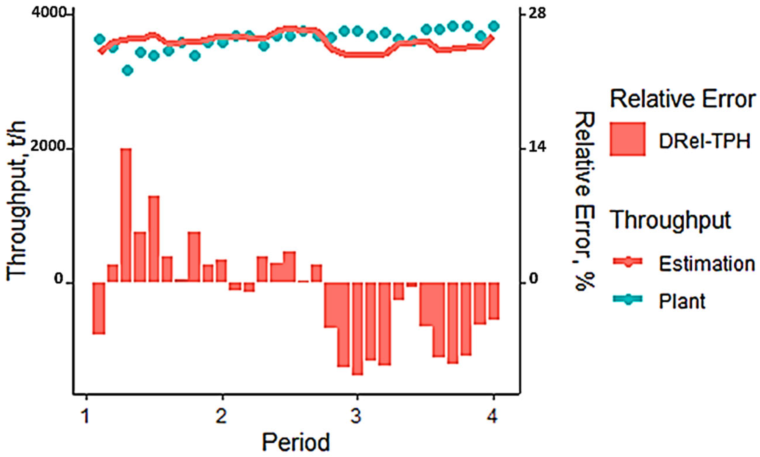
Figure 24 shows the reconciliation between actual plant throughput and estimates from the predictive model based on the Standard Grindability Index (SGI) combined with the Bond Work Index (BWi). This comparison evaluates the SGI-BWi model’s ability to replicate operational throughput behavior across different production periods.

The graph includes two vertical axes: the left axis represents throughput in tons per hour (t/h), and the right axis shows relative error as a percentage. Bars represent estimated and actual throughput values, while the relative error line illustrates the magnitude and direction of deviations.

Across the analyzed periods, at least three instances show significant divergence between model estimates and observed plant values. These discrepancies suggest that under certain operational conditions or ore characteristics, the SGI-BWi model fails to adequately capture system dynamics, indicating limitations in generalization or parameter representativeness.

Quantitatively, the model yields an RMSE of 219 t/h, a considerable deviation compared to other models in this study. While it may provide a general approximation of system behavior, its precision is limited and may not be suitable for applications requiring high predictive fidelity, such as short-term planning or real-time optimization.

It is important to note that the SGI-BWi model’s performance may be influenced by multiple factors, including mineralogical variability, grinding circuit conditions, and sensitivity to input parameters. Therefore, it is recommended to complement this approach with additional models or more robust calibration techniques, especially when aiming for reliable decision-making tools in high-variability operational contexts.

4. Discussion

The comparative evaluation of predictive models for estimating processing capacity (TPH) in the context of mineral processing is a critical component in the optimization of industrial operations. In this study, three approaches based on combinations of comminution indices were analyzed: DWi-BWi, SMC-BWi (the Morrell power model), and SGI-BWi. Each of these models exhibits distinct characteristics in terms of computational complexity, predictive accuracy, and statistical robustness.

4.1. The DWi-BWi Model: Dual Processing and Optimization

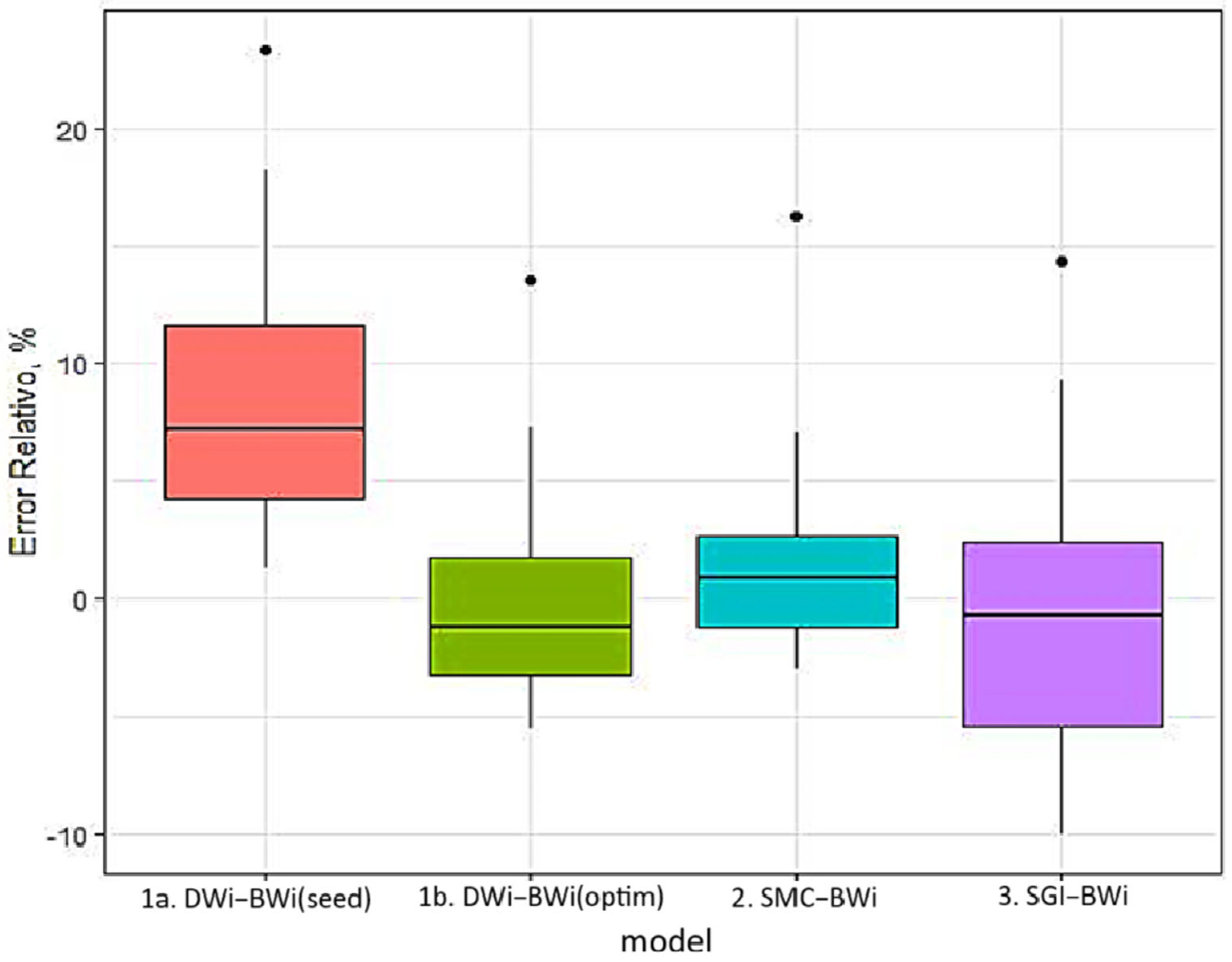
The DWi-BWi model is implemented in two stages: an initial phase based on seed values and a subsequent optimization phase. This dual-processing structure entails additional computational load but allows for parameter refinement to enhance predictive performance. In its initial form (DWi-BWi seed), the model yields a relatively high root mean square error (RMSE = 351 t/h), indicating poor fitting capability without calibration. However, after optimization, the RMSE is significantly reduced to 147 t/h, demonstrating the effectiveness of the tuning process in improving model performance.

From a statistical perspective, the optimized model exhibits a mean relative error close to zero (−0.0382) and a standard deviation of 4.19, suggesting virtually no bias and moderate variability. Nevertheless, this improvement is accompanied by the risk of overfitting, particularly when the model is trained on a limited or non-representative dataset. Such overfitting may compromise the model’s generalization capacity in operational scenarios different from those used during calibration.

4.2. The SMC-BWi Model: Simplicity and Accuracy

The Morrell power model (SMC-BWi) stands out for its structural simplicity and high predictive accuracy. With an RMSE of 143 t/h, it is the model with the lowest root mean square error among those evaluated. Additionally, it presents a mean relative error of 1.5% with a standard deviation of 3.92, indicating low bias and controlled dispersion. Unlike the DWi-BWi model, the SMC-BWi does not require a post-optimization phase, making it an efficient and reliable tool for real-time industrial applications.

From an operational standpoint, the absence of a tuning phase significantly reduces implementation time and computational requirements. This makes it particularly attractive for processing plants that demand fast and robust decision-making tools.

4.3. The SGI-BWi Model: High Variability and Predictive Limitations

Although conceptually valid, the SGI-BWi model presents significant limitations in terms of accuracy and stability. With an RMSE of 219 t/h, its performance is inferior to that of the other models. Furthermore, it exhibits a mean relative error of −1.18% with a standard deviation of 5.91, indicating a negative bias and high variability in predictions. This dispersion suggests that the model is more sensitive to fluctuations in input data, which may be due to the lower representativeness of the SGI index in the energy dynamics of the comminution process (

Table 4. Descriptive Statistics, Relative Errors, and RMSE for TPH Estimation.

Model	N (Samples)	Mean	Standard Deviation	Min	Max	RMSE
1a. DWi-BWi (seed)	30	8.34	5.32	1.35	23.3	351
1b. DWi-BWi (optimized)	30	−0.0382	4.19	−5.48	13.5	147
2. SMC-BWi	30	1.5	3.92	−2.97	16.3	143
3. SGI-BWi	30	−1.18	5.91	−10	14.3	219

).

4.4. Graphical Comparison and Analysis of Relative Errors

Figure 25 provides a visual comparison of the relative error behavior across the three models. It can be observed that the optimized DWi-BWi model achieves a significant reduction in error compared to its initial version, approaching the performance of the SMC-BWi model. However, its reliance on a post-tuning process introduces uncertainty regarding its long-term stability. In contrast, the SGI-BWi model shows greater dispersion in its relative errors, reinforcing its lower reliability as a predictive tool.

4.5. Selection of the Optimal Model

The selection of the optimal model is based on two main criteria: root mean square error (RMSE) and relative error behavior. According to these criteria, the Morrell power model (SMC-BWi) emerges as the most suitable alternative for estimating processing capacity. Its low RMSE, reduced bias, and statistical stability make it a robust, accurate, and easy-to-implement tool. Moreover, its independence from additional calibration processes makes it ideal for dynamic operational environments where speed and reliability are essential.

5. Conclusions

This study evaluated three alternative models for predicting throughput in the SAG-ball mill circuit at Antapaccay Mine, based on different combinations of comminution indices. Among the evaluated approaches, the model integrating SMC parameters (Mia, Mib) with the Bond Work Index (BWi) demonstrated the highest predictive accuracy, achieving the lowest root mean square error (RMSE = 143 t/h) and a mean relative error of 1.5%.

The modeling process incorporated a comprehensive dataset, including monthly mining volumes, hourly plant operational data, and metallurgical test results (JKDWT and BWi), filtered to ensure steady-state operating conditions. This methodological rigor enhances the model’s reliability and applicability within the operational context of Antapaccay Mine.

Although the SMC-BWi model was calibrated using site-specific data, its structure is generalizable and can be adapted to other mining operations. However, direct application without calibration is not recommended due to differences in ore mineralogy, circuit configuration, and operational constraints. Site-specific calibration using local comminution test data and operational records is essential to ensure predictive accuracy and model robustness.

From an economic perspective, the implementation of this model contributes to operational efficiency by enabling more accurate throughput forecasting. This facilitates better alignment between mine planning and plant capacity, reducing the risk of overloading or underutilization. Furthermore, the model supports the development of integrated comminution–flotation simulations, which can anticipate the impact of changes in feed characteristics or circuit design. These capabilities translate into improved resource allocation, reduced energy consumption per ton processed, and enhanced metallurgical recovery—ultimately contributing to the economic sustainability of the operation.

In summary, the SMC−BWi model not only provides a reliable tool for throughput prediction at Antapaccay Mine but also offers a transferable modeling strategy that, with appropriate calibration, can be adapted to other mining contexts. Its integration into geometallurgical workflows represents a valuable contribution to the optimization of mineral processing operations and the economic performance of mining facilities.