
Application of Soft Computing, Statistical and Multi-Criteria Decision-Making Methods to Develop a Predictive Equation for Prediction of Flyrock Distance in Open-Pit Mining

 ,
,  and
and
Abstract
1. Introduction and Background of Study
- The presence of pebbles around blast holes as a result of drilling;
- The lack of consideration of the delay sequence in blast holes;
- The presence of weak layers in the superficial layers of the ground.
- Choosing improper explosives by disregarding the geological conditions and properties of the rock mass;
- Using an improper drilling pattern and having inaccuracies in execution.
2. Related Work and Objective of This Study
3. The Case Study of Jajarm Bauxite Mine
3.1. Site Description
3.2. Data Sets
4. Methodology
4.1. Regression Analysis
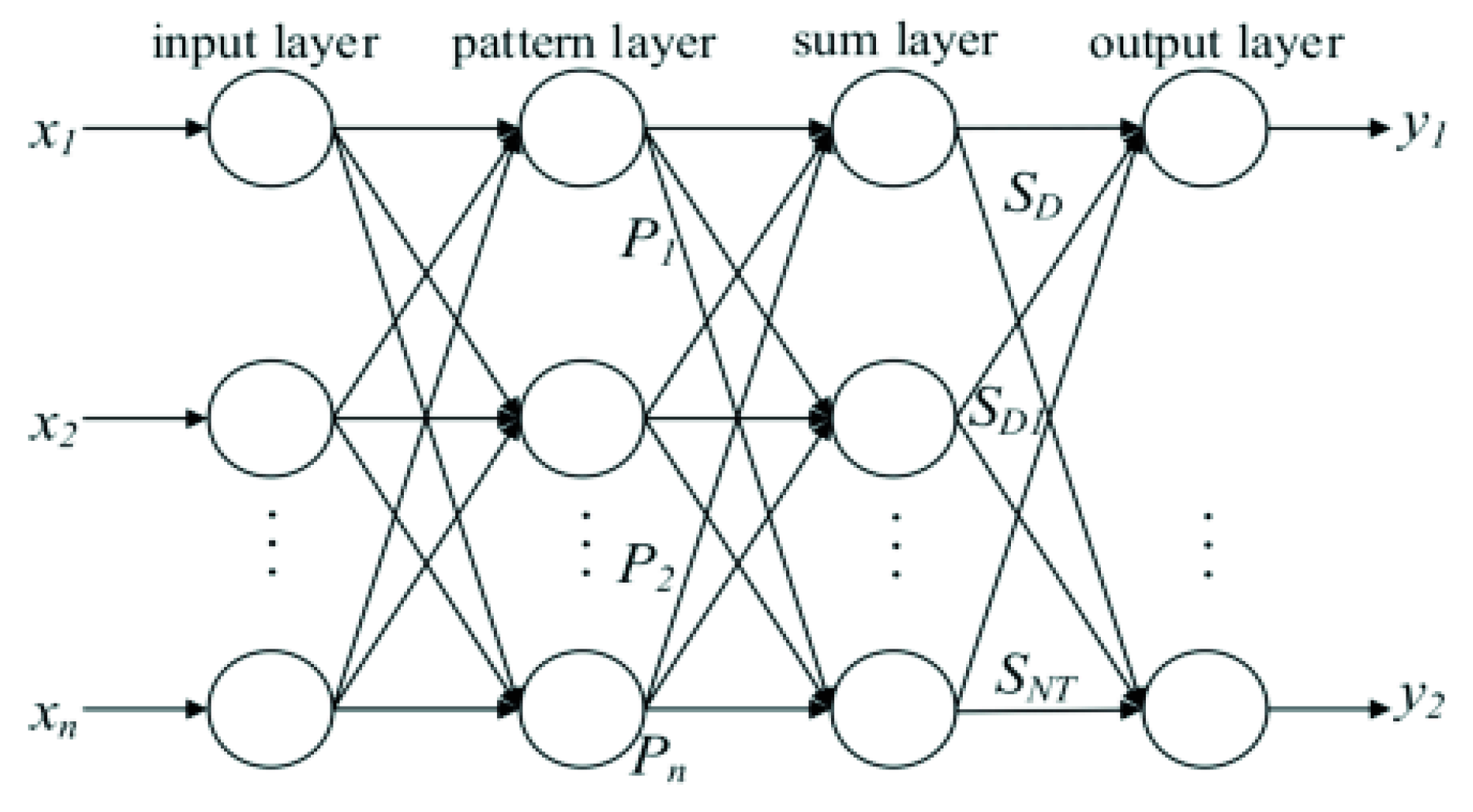
4.2. Generalized Regression Neural Network (GRNN)
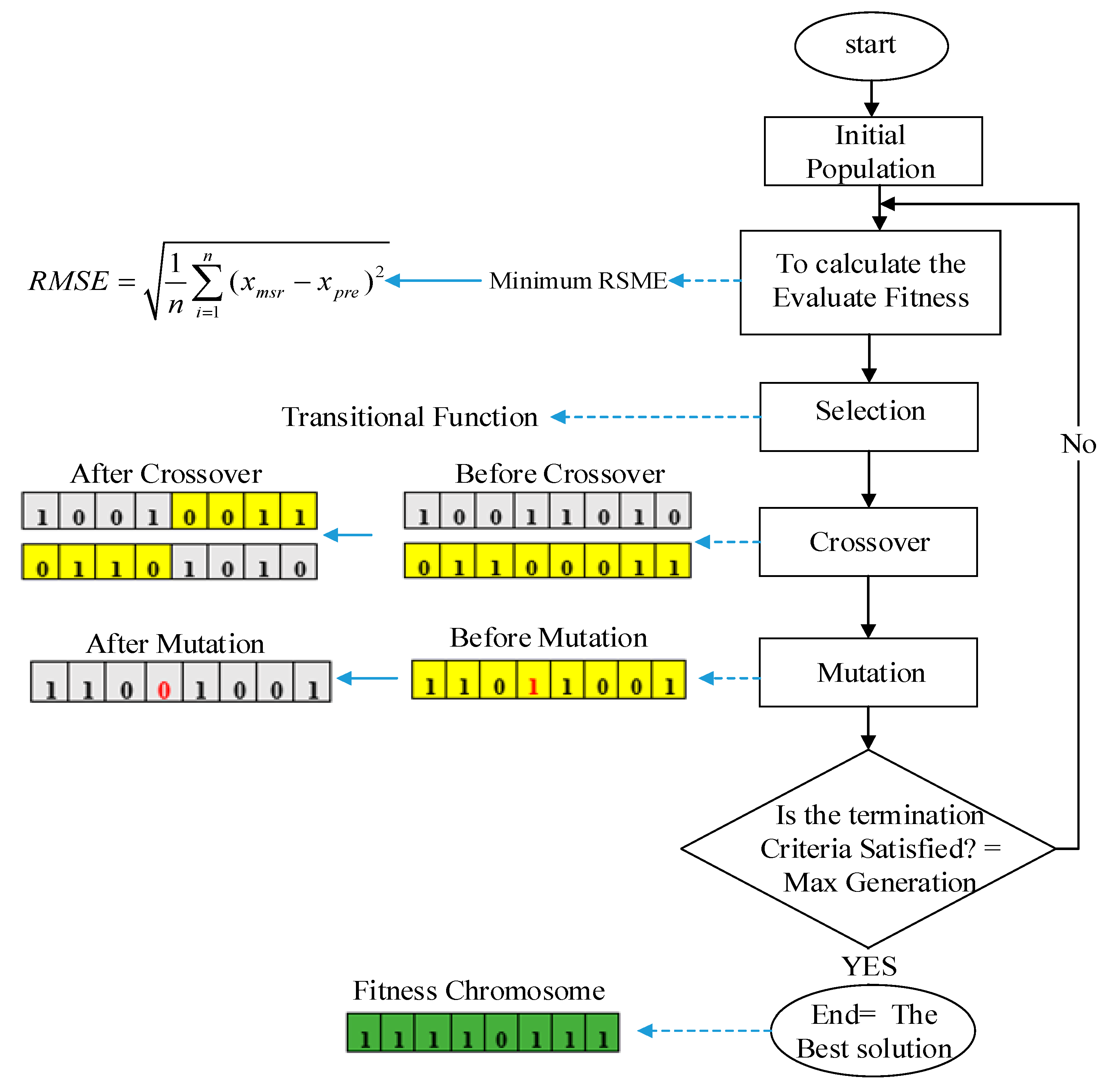
4.3. Genetic Algorithm (GA)
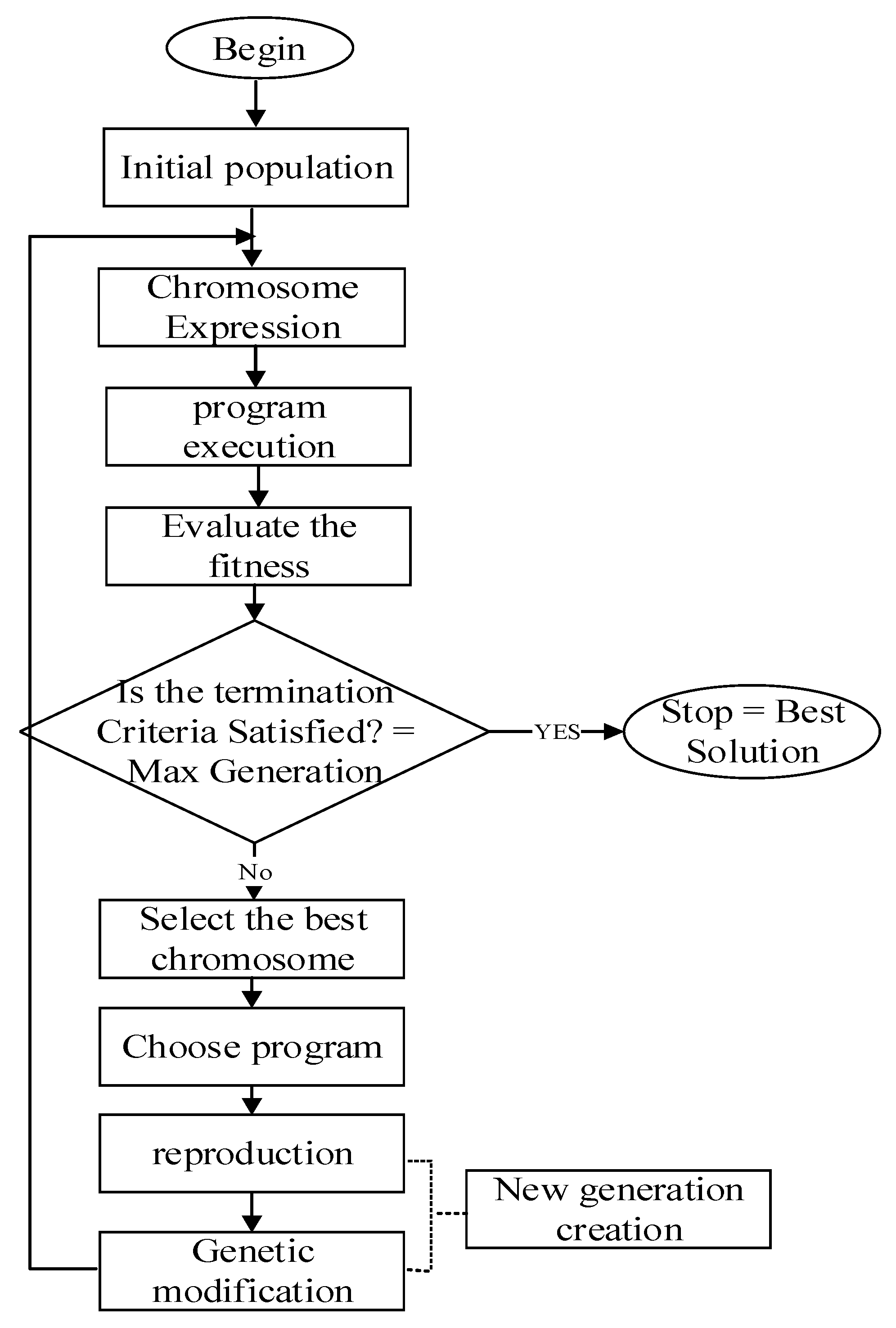
4.4. Gene Expression Programming (GEP)
4.5. Fuzzy DEMATEL Technique
5. Development of Predictive Models
5.1. Regression Model
5.2. GRNN Model
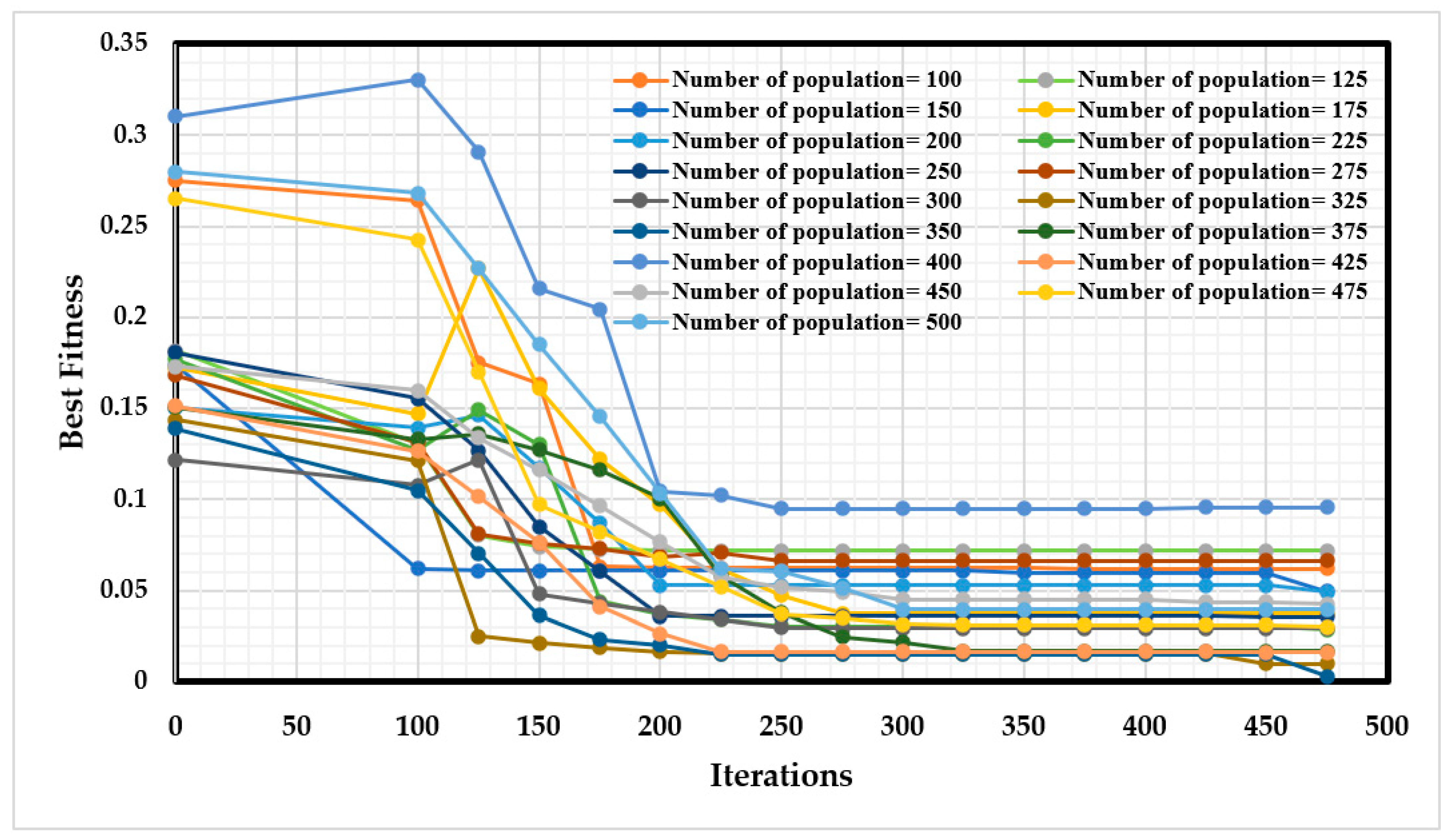
5.3. GA-GRNN Model
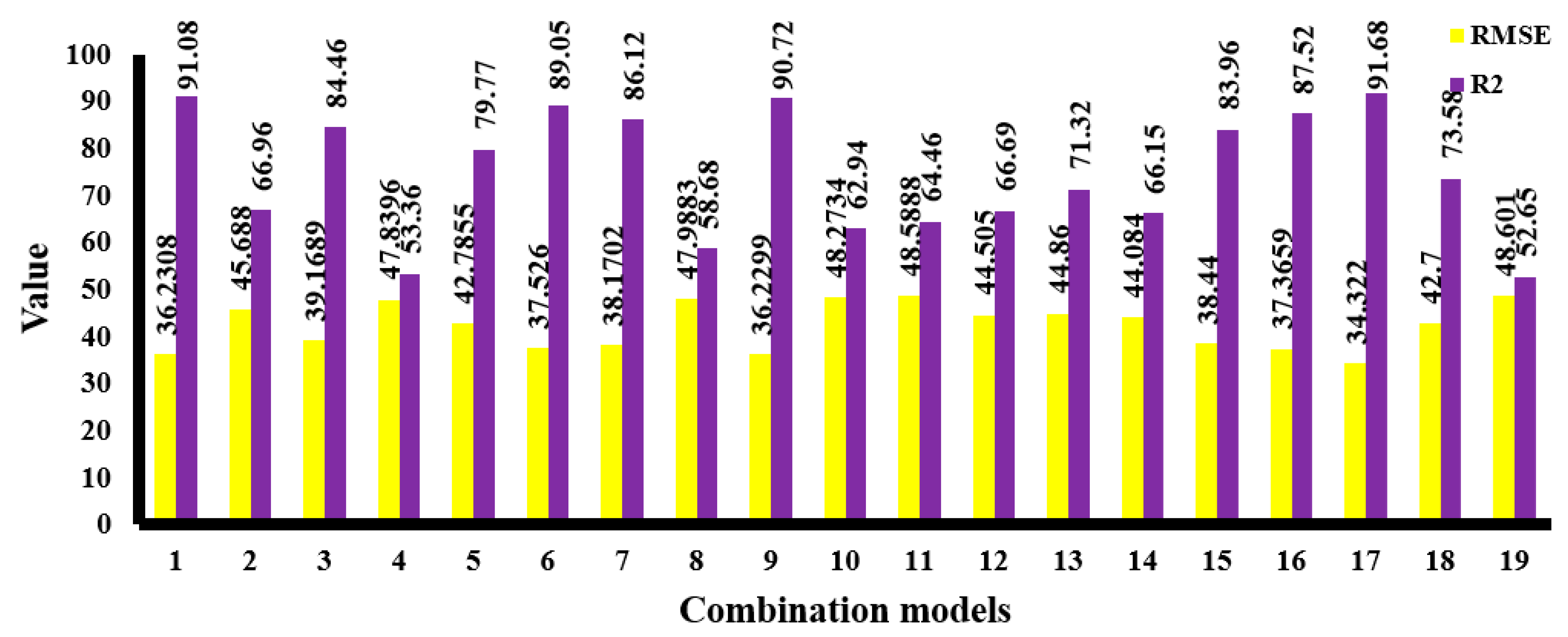
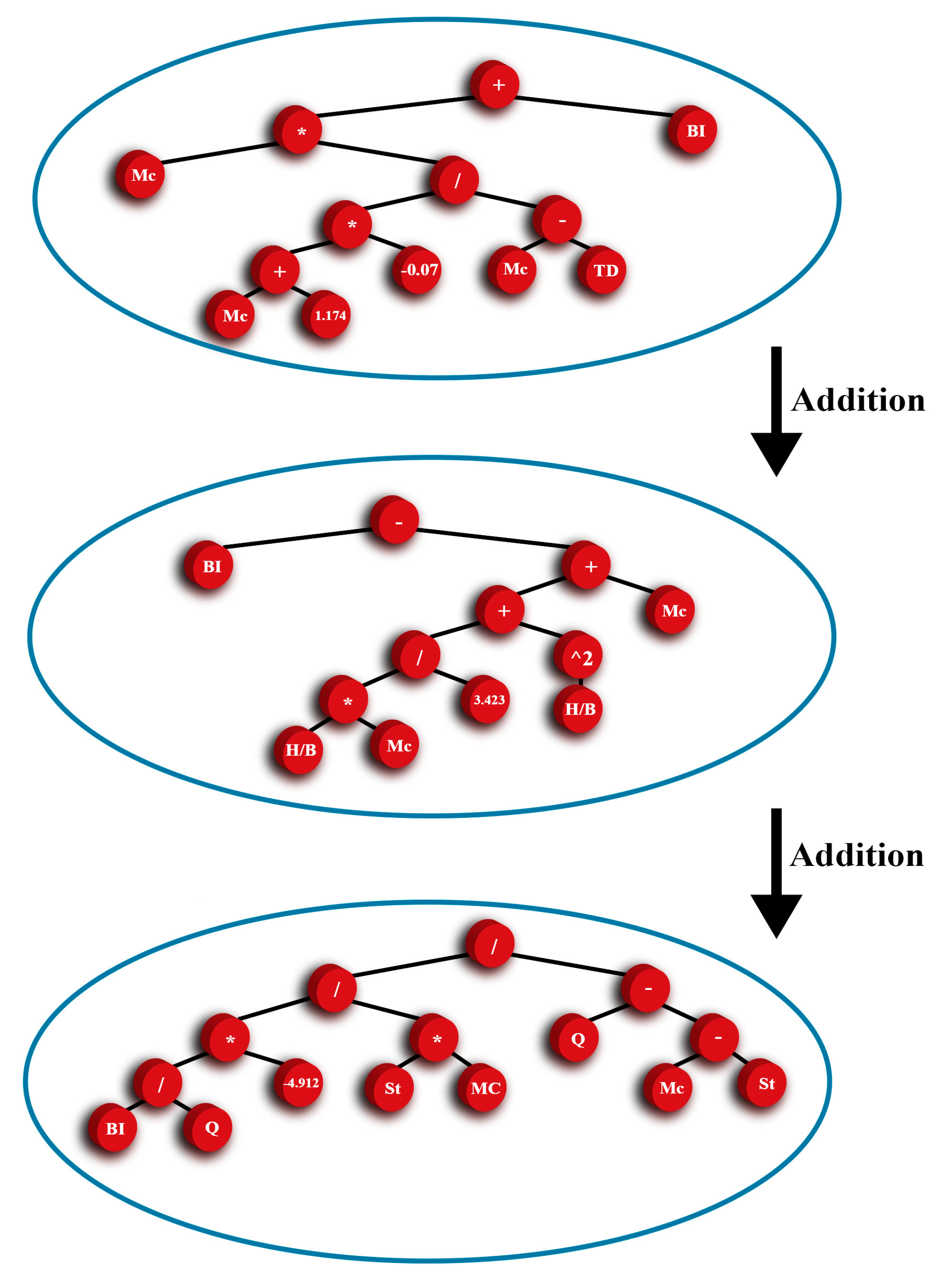
5.4. GEP Model
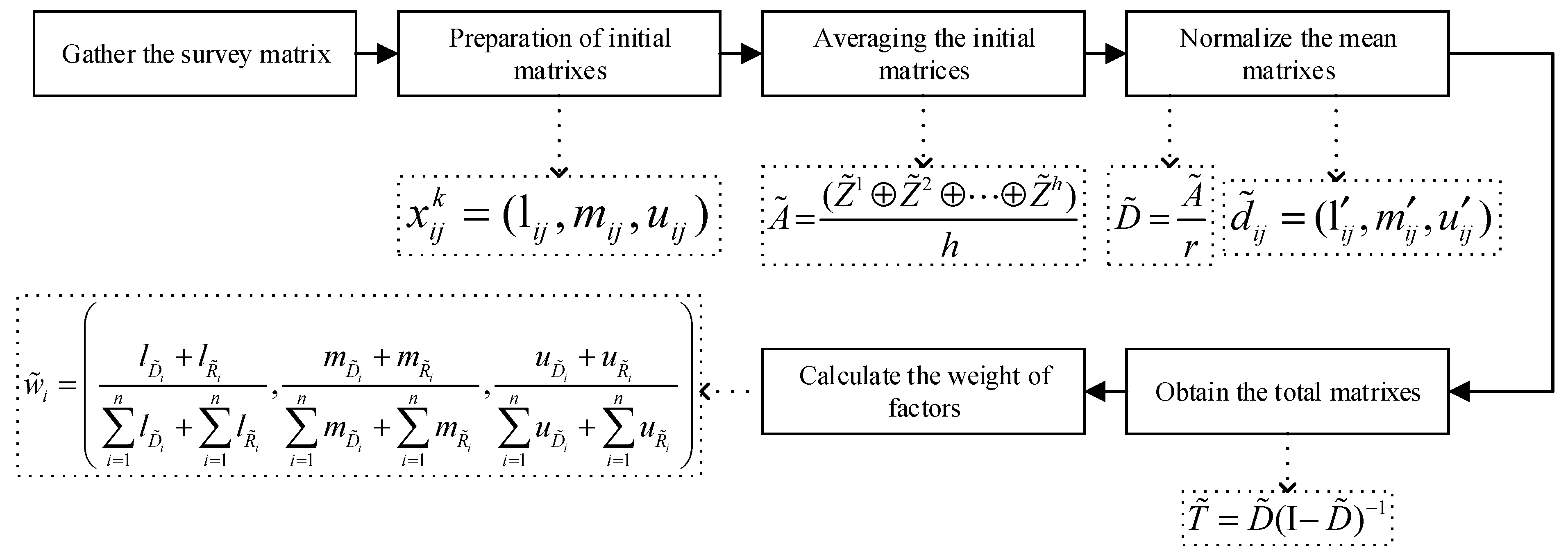
5.5. Fuzzy DEMATEL Model
Proposed Fuzzy DEMATEL Method
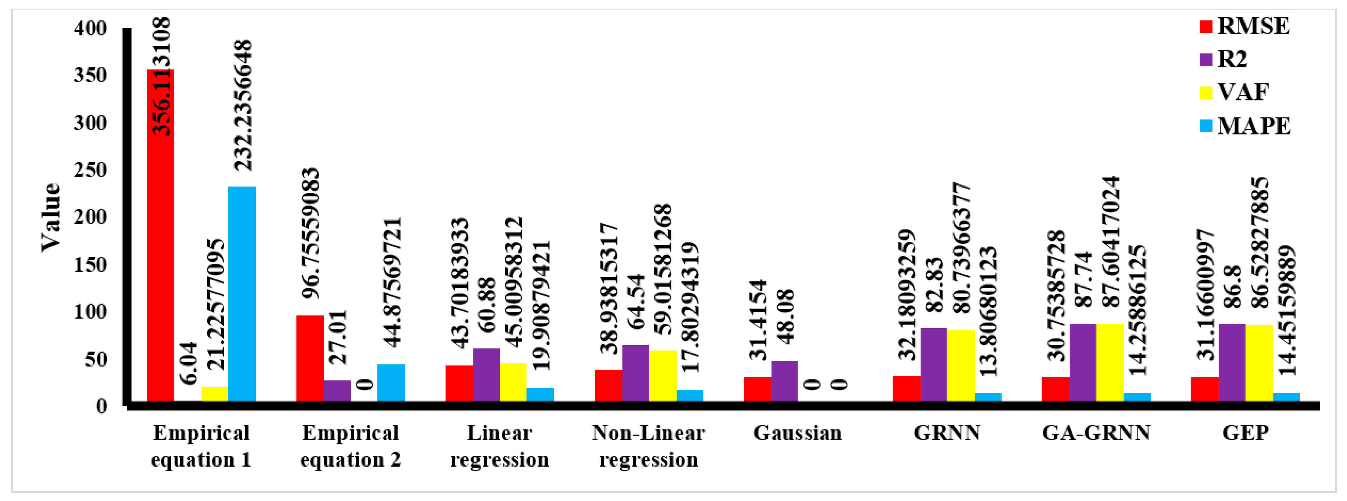
6. Evaluation of Proposed Models
7. Conclusions
- Multivariable linear and nonlinear regression methods were used in the statistical approach, and the best performance of linear regression, with effective parameters including Mc, Pf, S/B, H/B and HDEV, had R2 = 96.01 and RMSE = 11.46 in training and R2 = 60.88, RMSE = 43.701, VAF = 45.009 and MAPE = 19.908 on the test data. Additionally, with the same effective parameters, nonlinear regression had R2 = 89.5 and RMSE = 8.5 in data training and R2 = 64.54, RMSE = 38.938, VAF = 59.015 and MAPE = 17.802 on the test data.
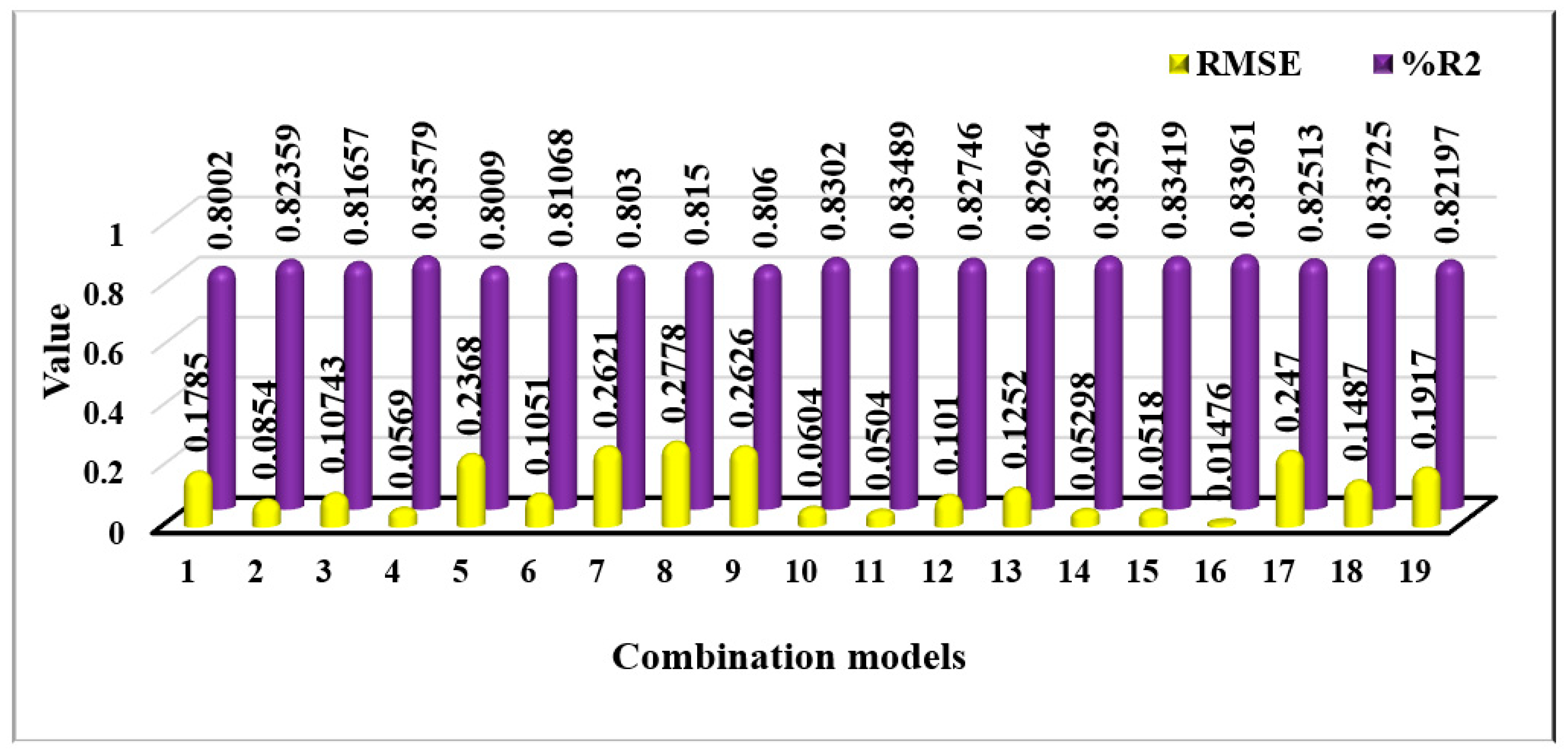
- The best models were produced by the soft computing method. In the GRNN method, the effective parameters were Mc, S/B, H/B, TD, BI and St, and in the GEP method, the effective parameters were Mc, H/B, TD, BI, Q and St. Three methods were used in this approach as follows:
- The first, the generalized regression neural network, was applied to data with Euclidean distance = 9.9, R2 = 83.961 and RMSE = 0.01476 in training and R2 = 82.83, RMSE = 32.1809, VAF = 80.739 and MAPE = 13.806 on the test data.
- GA-GRNN was the second method, which had R2 = 88.68 and RMSE = 0.0151 in training and R2 = 87.74, RMSE = 30.753, VAF = 87.604 and MAPE = 14.258 on the test data.
- Gene expression programming was another soft computing method applied to the different combinations of parameters. The best performance of this method was R2 = 91.68 and RMSE = 34.32 on the training data and R2 = 86.8, RMSE = 31.166, VAF = 86.528 and MAPE = 14.451 on the test data.
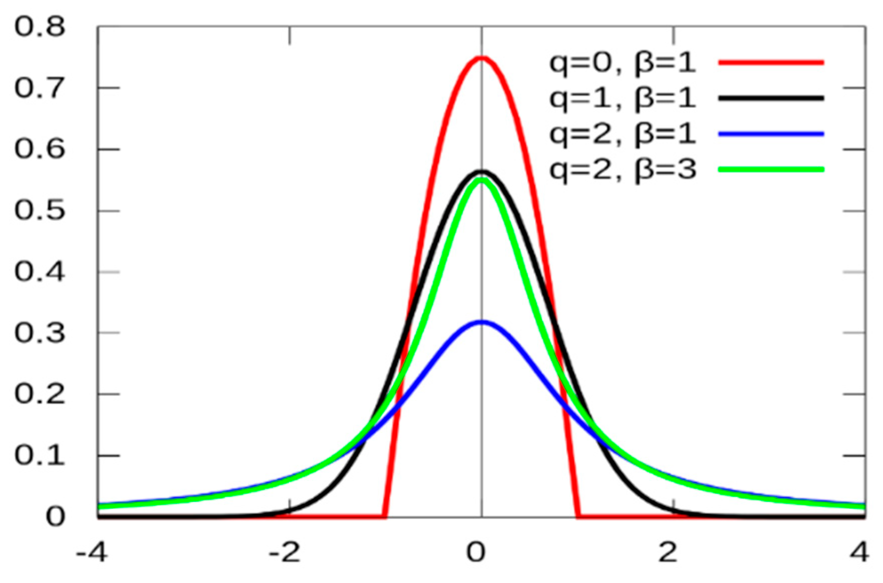
- Fuzzy DEMATEL was the last approach applied to the parameters affecting flyrock. In this regard, the amount of flyrock was predicted based on the function of the flyrock, the best of which was a Gaussian function. The performance of this function on the training data was R2 = 87.171, RMSE = 34.682. In addition, its performance was R2 = 48.08 and RMSE = 31.415 on the test data.
- Finally, the best models obtained from each method were selected and evaluated and compared to each other. The results of these evaluations showed that the GA-GRNN model’s performance was far better compared to others and has reasonable conformity to actual values due to its higher VAF and lower MAPE and RMSE, and it represents a direct practical equation.
Author Contributions
Funding
Data Availability Statement
Conflicts of Interest
References
- Sanchidrián, J.A.; Segarra, P.; López, L.M. Energy components in rock blasting. Int. J. Rock Mech. Min. Sci. 2007, 44, 130–147. [Google Scholar] [CrossRef]
- Singh, T.; Singh, V. An intelligent approach to prediction and controlground vibration in mines. Geotech. Geol. Eng. 2005, 23, 249–262. [Google Scholar] [CrossRef]
- Institute of Makers of Explosives (IME). Glossary of Commercial Explosives Industry Terms; Safety Library: Washington, DC, USA, 1997; p. 16. [Google Scholar]
- Kecojevic, V.; Radomsky, M. Flyrock phenomena and area security in blasting-related accidents. Saf. Sci. 2005, 43, 739–750. [Google Scholar] [CrossRef]
- Monjezi, M.; Mehrdanesh, A.; Malek, A.; Khandelwal, M. Evaluation of effect of blast design parameters on flyrock using artificial neural networks. Neural Comput. Appl. 2013, 23, 349–356. [Google Scholar] [CrossRef]
- Faramarzi, F.; Mansouri, H.; Farsangi, M.A.E. Development of rock engineering systems-based models for flyrock risk analysis and prediction of flyrock distance in surface blasting. Rock Mech. Rock Eng. 2014, 47, 1291–1306. [Google Scholar] [CrossRef]
- Hustrulid, W.A. Blasting Principles for Open Pit Mining: General Design Concepts; Balkema: Boca Raton, FL, USA, 1999. [Google Scholar]
- Bajpayee, T.; Rehak, T.; Mowrey, G.; Ingram, D. Blasting injuries in surface mining with emphasis on flyrock and blast area security. J. Saf. Res. 2004, 35, 47–57. [Google Scholar] [CrossRef]
- Aghajani-Bazzazi, A.; Osanloo, M.; Azimi, Y. Flyrock prediction by multiple regression analysis in Esfordi phosphate mine of Iran. In Proceedings of the 9th International Symposium on Rock Fragmentation by Blasting, Granada, Spain, 13–17 August 2009; pp. 649–657. [Google Scholar]
- Armaghani, D.J.; Hajihassani, M.; Mohamad, E.T.; Marto, A.; Noorani, S. Blasting-induced flyrock and ground vibration prediction through an expert artificial neural network based on particle swarm optimization. Arab. J. Geosci. 2014, 7, 5383–5396. [Google Scholar] [CrossRef]
- Faradonbeh, R.S.; Jahed Armaghani, D.; Monjezi, M. Development of a new model for predicting flyrock distance in quarry blasting: A genetic programming technique. Bull. Eng. Geol. Environ. 2016, 75, 993–1006. [Google Scholar] [CrossRef]
- Han, H.; Jahed Armaghani, D.; Tarinejad, R.; Zhou, J.; Tahir, M. Random forest and bayesian network techniques for probabilistic prediction of flyrock induced by blasting in quarry sites. Nat. Resour. Res. 2020, 29, 655–667. [Google Scholar] [CrossRef]
- Trivedi, R.; Singh, T.; Gupta, N. Prediction of blast-induced flyrock in opencast mines using ANN and ANFIS. Geotech. Geol. Eng. 2015, 33, 875–891. [Google Scholar] [CrossRef]
- Fouladgar, N.; Hasanipanah, M.; Bakhshandeh Amnieh, H. Application of cuckoo search algorithm to estimate peak particle velocity in mine blasting. Eng. Comput. 2017, 33, 181–189. [Google Scholar] [CrossRef]
- Hasanipanah, M.; Jahed Armaghani, D.; Bakhshandeh Amnieh, H.; Majid, M.Z.A.; Tahir, M.M. Application of PSO to develop a powerful equation for prediction of flyrock due to blasting. Neural Comput. Appl. 2017, 28, 1043–1050. [Google Scholar] [CrossRef]
- Khandelwal, M.; Monjezi, M. Prediction of backbreak in open-pit blasting operations using the machine learning method. Rock Mech. Rock Eng. 2013, 46, 389–396. [Google Scholar] [CrossRef]
- Yang, H.; Hasanipanah, M.; Tahir, M.; Bui, D.T. Intelligent prediction of blasting-induced ground vibration using ANFIS optimized by GA and PSO. Nat. Resour. Res. 2020, 29, 739–750. [Google Scholar] [CrossRef]
- Richards, A.; Moore, A. Flyrock control-by chance or design. In Proceedings of the Annual Conference on Explosives and Blasting Technique, New Orleans, LA, USA, 1–4 February 2004. [Google Scholar]
- Marto, A.; Hajihassani, M.; Jahed Armaghani, D.; Tonnizam Mohamad, E.; Makhtar, A.M. A novel approach for blast-induced flyrock prediction based on imperialist competitive algorithm and artificial neural network. Sci. World J. 2014, 2014, 643715. [Google Scholar] [CrossRef] [PubMed]
- Little, T. Flyrock risk. In Proceedings of the EXPLO, Wollongong, Australia, 3–4 September 2007. [Google Scholar]
- Bhandari, S. Engineering Rock Blasting Operations; Taylor & Francis: London, UK, 1997. [Google Scholar]
- Jimeno, C.L.; Jimeno, E.L.; Carcedo, F.J.A.; de Ramiro, Y.V. Drilling änd Blasting of Rocks; Routledge: Abingdon-on-Thames, UK, 1995. [Google Scholar]
- Ladegaard-Pedersen, A.; Holmberg, R. The Dependence of Charge Geometry on Flyrock Caused by Crater Effects in Bench Blasting; Report DS; Swedish Detonic Research Foundation: Kiruna, Sweden, 1973; pp. 1–38. [Google Scholar]
- Langefors, U.; Kihlstrom, B. The Modern Techniques of Rock Blasting; John Wiely and Sons, Inc.: New York, NY, USA, 1978; p. 438. [Google Scholar]
- Lundborg, N.; Persson, A.; Ladegaard-Pedersen, A.; Holmberg, R. Keeping the lid on flyrock in open-pit blasting. Eng. Min. J. 1975, 176, 95–100. [Google Scholar]
- Lundborg, N. The Probability of Flyrock; SveDeFo: Stockholm, Sweden, 1981. [Google Scholar]
- Kopp, J. Observation of Flyrock at Several Mines and Quarries; International Society of Explosives Engineers: Cleveland, OH, USA, 1994. [Google Scholar]
- Bajpayee, T.; Rehak, T.; Mowrey, G.; Ingram, D. A summary of fatal accidents due to flyrock and lack of blast area security in surface mining, 1989 to 1999. In Proceedings of the Twenty-Eighth Annual Conference on Explosives and Blasting Technique, Las Vegas, NV, USA, 10–13 February 2002. [Google Scholar]
- Verakis, H.; Lobb, T. An analysis of blasting accidents in mining operations. In Proceedings of the Annual Conference on Explosives and Blasting Technique, Prague, Czech Republic, 10–12 September 2003. [Google Scholar]
- Workman, J.; Calder, P. Flyrock Prediction and Control in Surface Mine Blasting; International Society of Explosives Engineers: Cleveland, OH, USA, 1994. [Google Scholar]
- Monjezi, M.; Dehghan, J.A.H.; Samimi, N.F. Application of TOPSIS method in controlling fly rock in blasting operations. In Proceedings of the 7th International Multidisciplinary Scientific Geoconference Sgem, Albena, Bulgaria, 11–15 June 2007. [Google Scholar]
- Rezaei, M.; Monjezi, M.; Varjani, A.Y. Development of a fuzzy model to predict flyrock in surface mining. Saf. Sci. 2011, 49, 298–305. [Google Scholar] [CrossRef]
- Monjezi, M.; Bahrami, A.; Varjani, A.; Sayadi, A. Prediction and controlling of flyrock in blasting operation using artificial neural network. Arab. J. Geosci. 2011, 4, 421–425. [Google Scholar] [CrossRef]
- Monjezi, M.; Amini Khoshalan, H.; Yazdian Varjani, A. Prediction of flyrock and backbreak in open pit blasting operation: A neuro-genetic approach. Arab. J. Geosci. 2012, 5, 441–448. [Google Scholar] [CrossRef]
- Amini, H.; Gholami, R.; Monjezi, M.; Torabi, S.R.; Zadhesh, J. Evaluation of flyrock phenomenon due to blasting operation by support vector machine. Neural Comput. Appl. 2012, 21, 2077–2085. [Google Scholar] [CrossRef]
- Ghasemi, E.; Amini, H.; Ataei, M.; Khalokakaei, R. Application of artificial intelligence techniques for predicting the flyrock distance caused by blasting operation. Arab. J. Geosci. 2014, 7, 193–202. [Google Scholar] [CrossRef]
- Saghatforoush, A.; Monjezi, M.; Shirani Faradonbeh, R.; Jahed Armaghani, D. Combination of neural network and ant colony optimization algorithms for prediction and optimization of flyrock and back-break induced by blasting. Eng. Comput. 2016, 32, 255–266. [Google Scholar] [CrossRef]
- Esen, S. Effective fragmentation and flyrock control strategies at quarries. Int. J. Econ. Environ. Geol. 2017, 8, 20–28. [Google Scholar]
- Armaghani, D.J.; Koopialipoor, M.; Bahri, M.; Hasanipanah, M.; Tahir, M. A SVR-GWO technique to minimize flyrock distance resulting from blasting. Bull. Eng. Geol. Environ. 2020, 79, 4369–4385. [Google Scholar] [CrossRef]
- Hasanipanah, M.; Bakhshandeh Amnieh, H. A fuzzy rule-based approach to address uncertainty in risk assessment and prediction of blast-induced Flyrock in a quarry. Nat. Resour. Res. 2020, 29, 669–689. [Google Scholar] [CrossRef]
- Lu, X.; Hasanipanah, M.; Brindhadevi, K.; Bakhshandeh Amnieh, H.; Khalafi, S. ORELM: A novel machine learning approach for prediction of flyrock in mine blasting. Nat. Resour. Res. 2020, 29, 641–654. [Google Scholar] [CrossRef]
- Nikafshan Rad, H.; Bakhshayeshi, I.; Wan Jusoh, W.A.; Tahir, M.; Foong, L.K. Prediction of flyrock in mine blasting: A new computational intelligence approach. Nat. Resour. Res. 2020, 29, 609–623. [Google Scholar] [CrossRef]
- Zhou, J.; Aghili, N.; Ghaleini, E.N.; Bui, D.T.; Tahir, M.; Koopialipoor, M. A Monte Carlo simulation approach for effective assessment of flyrock based on intelligent system of neural network. Eng. Comput. 2020, 36, 713–723. [Google Scholar] [CrossRef]
- Jamei, M.; Hasanipanah, M.; Karbasi, M.; Ahmadianfar, I.; Taherifar, S. Prediction of flyrock induced by mine blasting using a novel kernel-based extreme learning machine. J. Rock Mech. Geotech. Eng. 2021, 13, 1438–1451. [Google Scholar] [CrossRef]
- Monjezi, M.; Dehghani, H.; Shakeri, J.; Mehrdanesh, A. Optimization of prediction of flyrock using linear multivariate regression (LMR) and gene expression programming (GEP)—Topal Novin mine, Iran. Arab. J. Geosci. 2021, 14, 1483. [Google Scholar] [CrossRef]
- Nguyen, H.; Bui, X.-N.; Choi, Y.; Lee, C.W.; Armaghani, D.J. A novel combination of whale optimization algorithm and support vector machine with different kernel functions for prediction of blasting-induced fly-rock in quarry mines. Nat. Resour. Res. 2021, 30, 191–207. [Google Scholar] [CrossRef]
- Shakeri, J.; Amini Khoshalan, H.; Dehghani, H.; Bascompta, M.; Onyelowe, K. Developing new models for flyrock distance assessment in open-pit mines. J. Min. Environ. 2022, 13, 375–389. [Google Scholar]
- Hudaverdi, T. Prediction of flyrock throw distance in quarries by variable selection procedures and ANFIS modelling technique. Environ. Earth Sci. 2022, 81, 281. [Google Scholar] [CrossRef]
- Hosseini, S.; Poormirzaee, R.; Hajihassani, M.; Kalatehjari, R. An ANN-fuzzy cognitive map-based Z-number theory to predict flyrock induced by blasting in open-pit mines. Rock Mech. Rock Eng. 2022, 55, 4373–4390. [Google Scholar] [CrossRef]
- Barkhordari, M.; Armaghani, D.; Fakharian, P. Ensemble machine learning models for prediction of flyrock due to quarry blasting. Int. J. Environ. Sci. Technol. 2022, 19, 8661–8676. [Google Scholar] [CrossRef]
- Gupta, R. Surface blasting and its impact on environment. In Impact of Mining on Environment; Ashish Publishing House: New Delhi, India, 1980; pp. 23–24. [Google Scholar]
- Roy, P.P. Rock Blasting: Effects and Operations; CRC Press: Boca Raton, FL, USA, 2005. [Google Scholar]
- Ghasemi, E.; Sari, M.; Ataei, M. Development of an empirical model for predicting the effects of controllable blasting parameters on flyrock distance in surface mines. Int. J. Rock Mech. Min. Sci. 2012, 52, 163–170. [Google Scholar] [CrossRef]
- Trivedi, R.; Singh, T.; Raina, A. Prediction of blast-induced flyrock in Indian limestone mines using neural networks. J. Rock Mech. Geotech. Eng. 2014, 6, 447–454. [Google Scholar] [CrossRef]
- Babaeian, M.; Ataei, M.; Sereshki, F.; Sotoudeh, F.; Mohammadi, S. A new framework for evaluation of rock fragmentation in open pit mines. J. Rock Mech. Geotech. Eng. 2019, 11, 325–336. [Google Scholar] [CrossRef]
- Weisberg, S. Applied Linear Regression; John Wiley & Sons: Hoboken, NJ, USA, 2005; Volume 528. [Google Scholar]
- Tiryaki, B. Application of artificial neural networks for predicting the cuttability of rocks by drag tools. Tunn. Undergr. Space Technol. 2008, 23, 273–280. [Google Scholar] [CrossRef]
- Ghiasi, M.; Askarnejad, N.; Dindarloo, S.R.; Shamsoddini, H. Prediction of blast boulders in open pit mines via multiple regression and artificial neural networks. Int. J. Min. Sci. Technol. 2016, 26, 183–186. [Google Scholar] [CrossRef]
- Specht, D.F. A general regression neural network. IEEE Trans. Neural Netw. 1991, 2, 568–576. [Google Scholar] [CrossRef] [PubMed]
- Theodosiou, M. Disaggregation & aggregation of time series components: A hybrid forecasting approach using generalized regression neural networks and the theta method. Neurocomputing 2011, 74, 896–905. [Google Scholar]
- Santos, R.; Rupp, M.; Bonzi, S.; Fileti, A. Comparison between multilayer feedforward neural networks and a radial basis function network to detect and locate leaks in pipelines transporting gas. Chem. Eng. Trans. 2013, 32, 1375–1380. [Google Scholar]
- Hu, R.; Wen, S.; Zeng, Z.; Huang, T. A short-term power load forecasting model based on the generalized regression neural network with decreasing step fruit fly optimization algorithm. Neurocomputing 2017, 221, 24–31. [Google Scholar] [CrossRef]
- Ozyildirim, B.M.; Avci, M. Generalized classifier neural network. Neural Netw. 2013, 39, 18–26. [Google Scholar] [CrossRef]
- Bierkens, M.F. Modeling water table fluctuations by means of a stochastic differential equation. Water Resour. Res. 1998, 34, 2485–2499. [Google Scholar] [CrossRef]
- Lin, J.; Sheng, G.; Yan, Y.; Dai, J.; Jiang, X. Prediction of dissolved gas concentrations in transformer oil based on the KPCA-FFOA-GRNN model. Energies 2018, 11, 225. [Google Scholar] [CrossRef]
- Goldberg, D.E. Genetic Algorithms in Search, Optimization and Machine Learning; Addison Welssey Publishing Company: Reading, MA, USA, 1989. [Google Scholar]
- Khandelwal, M.; Armaghani, D.J. Prediction of drillability of rocks with strength properties using a hybrid GA-ANN technique. Geotech. Geol. Eng. 2016, 34, 605–620. [Google Scholar] [CrossRef]
- Daviran, M.; Maghsoudi, A.; Ghezelbash, R.; Pradhan, B. A new strategy for spatial predictive mapping of mineral prospectivity: Automated hyperparameter tuning of random forest approach. Comput. Geosci. 2021, 148, 104688. [Google Scholar] [CrossRef]
- Beiki, M.; Majdi, A.; Givshad, A.D. Application of genetic programming to predict the uniaxial compressive strength and elastic modulus of carbonate rocks. Int. J. Rock Mech. Min. Sci. 2013, 63, 159–169. [Google Scholar] [CrossRef]
- Mohamad, E.T.; Faradonbeh, R.S.; Armaghani, D.J.; Monjezi, M.; Majid, M.Z.A. An optimized ANN model based on genetic algorithm for predicting ripping production. Neural Comput. Appl. 2017, 28, 393–406. [Google Scholar] [CrossRef]
- Abhishek, K.; Panda, B.N.; Datta, S.; Mahapatra, S.S. Comparing predictability of genetic programming and ANFIS on drilling performance modeling for GFRP composites. Procedia Mater. Sci. 2014, 6, 544–550. [Google Scholar] [CrossRef]
- Ferreira, C. Gene expression programming: A new adaptive algorithm for solving problems. arXiv 2001, arXiv:cs/0102027. [Google Scholar]
- Brownlee, J. Clever Algorithms: Nature-Inspired Programming Recipes; Swinburne University of Technology: Melbourne, Australia, 2011. [Google Scholar]
- Steeb, W.-H. The Nonlinear Workbook: Chaos, Fractals, Cellular Automata, Neural Networks, Genetic Algorithms, Fuzzy Logic with C++, Java, Symbolicc++ and Reduce Programs; World Scientific: Singapore, 2002. [Google Scholar]
- Ferreira, C. Gene expression programming in problem solving. In Soft Computing and Industry: Recent Applications; Springer: Berlin/Heidelberg, Germany, 2002; pp. 635–653. [Google Scholar]
- Ferreira, C. Gene expression programming and the evolution of computer programs. In Recent Developments in Biologically Inspired Computing; IGI Global: Hershey, PA, USA, 2005; pp. 82–103. [Google Scholar]
- Ferreira, C. Gene Expression Programming: Mathematical Modeling by an Artificial Intelligence; Springer: Berlin/Heidelberg, Germany, 2006; Volume 21. [Google Scholar]
- Teodorescu, L.; Sherwood, D. High energy physics event selection with gene expression programming. Comput. Phys. Commun. 2008, 178, 409–419. [Google Scholar] [CrossRef]
- Rezaei, M. Forecasting the stress concentration coefficient around the mined panel using soft computing methodology. Eng. Comput. 2019, 35, 451–466. [Google Scholar] [CrossRef]
- Gabus, A.; Fontela, E. World Problems, an Invitation to Further Thought within the Framework of DEMATEL; Battelle Geneva Research Center: Geneva, Switzerland, 1972; Volume 1. [Google Scholar]
- Mohammadi, S.; Ataei, M.; Khaloo Kakaie, R.; Mirzaghorbanali, A. Prediction of the main caving span in longwall mining using fuzzy MCDM technique and statistical method. J. Min. Environ. 2018, 9, 717–726. [Google Scholar]
- Mohammadi, S.; Ataei, M.; Kakaie, R. Assessment of the importance of parameters affecting roof strata cavability in mechanized longwall mining. Geotech. Geol. Eng. 2018, 36, 2667–2682. [Google Scholar] [CrossRef]
- Suo, W.-L.; Feng, B.; Fan, Z.-P. Extension of the DEMATEL method in an uncertain linguistic environment. Soft Comput. 2012, 16, 471–483. [Google Scholar] [CrossRef]
- Lin, C.; Wu, W.-W. A fuzzy extension of the DEMATEL method for group decision making. Eur. J. Oper. Res. 2004, 156, 445–455. [Google Scholar]
- Jassbi, J.; Mohamadnejad, F.; Nasrollahzadeh, H. A Fuzzy DEMATEL framework for modeling cause and effect relationships of strategy map. Expert Syst. Appl. 2011, 38, 5967–5973. [Google Scholar] [CrossRef]
- Sangaiah, A.K.; Gopal, J.; Basu, A.; Subramaniam, P.R. An integrated fuzzy DEMATEL, TOPSIS, and ELECTRE approach for evaluating knowledge transfer effectiveness with reference to GSD project outcome. Neural Comput. Appl. 2017, 28, 111–123. [Google Scholar] [CrossRef]
- Mohammadi, S.; Babaeian, M.; Ataei, M.; Ghanbari, K. Quantifying roof falling potential based on CMRR method by incorporating DEMATEL-MABAC method; a case study. J. Min. Environ. 2021, 12, 151–162. [Google Scholar]
- Gokceoglu, C. A fuzzy triangular chart to predict the uniaxial compressive strength of the Ankara agglomerates from their petrographic composition. Eng. Geol. 2002, 66, 39–51. [Google Scholar] [CrossRef]
- Koopialipoor, M.; Fallah, A.; Armaghani, D.J.; Azizi, A.; Mohamad, E.T. Three hybrid intelligent models in estimating flyrock distance resulting from blasting. Eng. Comput. 2019, 35, 243–256. [Google Scholar] [CrossRef]
- Hudson, J. Rock Engineering Systems. Theory and Practice; Springer: Chicago, IL, USA, 1992. [Google Scholar]
- Rezaei, M. Development of an intelligent model to estimate the height of caving–fracturing zone over the longwall gobs. Neural Comput. Appl. 2018, 30, 2145–2158. [Google Scholar] [CrossRef]


| Mechanism of Flyrock | Prediction Model |
|---|---|
| Rifling | |
| Cratering | |
| Face bursting |
| Authors | Years | Findings |
|---|---|---|
| Ladegaard-Pedersen and Holmberg [23] | 1973 | The charging geometry affects cratering flyrock more than the other two types. |
| Langefors, and Kihlstrom [24] | 1978 | The flyrock distance increases as each blast hole’s main charge increases. |
| Lundborg [25,26] | 1981, 1975 | The first empirical model for flyrock prediction is presented. |
| Kopp [27] | 1994 | Flyrock makes up one-third of mining accidents. |
| Bajpayee et al. [28] | 2002 | A safe zone can be provided to prevent casualties and equipment damage. |
| Verakis and Lobb [29] | 2003 | The lack of consideration of geological conditions when choosing blasting patterns and explosives, improper stemming and charging and an unfit blasting sequence (blast hole’s delay) are influencing factors of flyrock. |
| Workman and Calder [30] | 1994 | |
| Kecojevic and Radomsky [4] | 2005 | Flyrock depends on factors such as geological structure, improper blasting pattern, the erroneous choice of burden, explosive aggregation, poor stemming and inaccuracy in choosing the correct blasting delay. |
| Monjezi et al. [31] | 2007 | The distance of flyrock in a blast was controlled using the Topsis method. |
| Aghajani-Bazzazi et al. [9] | 2009 | Controllable parameters were used to develop an empirical model to predict flyrock by using the multivariable regression method. |
| Rezaei et al. [32] | 2011 | Flyrock distance predictions based on the fuzzy method (FIS and artificial neural network) and the statistical method were compared. |
| Monjezi et al. [33] | 2011 | The ANNS method and its functionality were applied to predict the flyrock distance. |
| Monjezi et al. [34] | 2012 | The genetic neural network model was used to predict flyrock and backbreak. |
| Amini et al. [35] | 2012 | The results of flyrock distance prediction calculated through the SVM (support vector machine) method were compared to those obtained using the ANN (artificial neural network) method. |
| Ghasemi et al. [36] | 2014 | The functionality of the developed ANN method was compared to that of fuzzy logic in predicting the flyrock distance. |
| Armaghani et al. [10] | 2014 | A new combination method, Bp-Ann, was used to predict the flyrock distance and decrease the error rate. This method is a combination of the PSO (particle swarm optimization) algorithm and the ANN (artificial neural network) function. |
| Faramarzi et al. [6] | 2014 | The functionality of the multivariable regression method was compared with the rock engineering system (RES) in predicting the flyrock distance. |
| Saghatforoush et al. [37] | 2016 | Ant colony and optimization algorithms were used to predict the flyrock distance and backbreak, which eventually led to a new ACO method for minimizing flyrock distance and backbreak. |
| Esen [38] | 2017 | The flyrock distance was predicted with the aim of determining the safe zone in open-pit mines using the effects of parameters on flyrock. |
| Hasanipanah et al. [15] | 2017 | The PSO (particle swarm optimization) method was applied, and its results were compared to those of Multiple Linear Regression (MLR) in predicting the flyrock distance. |
| Armaghani et al. [39] | 2020 | Three different methods of machine learning techniques, i.e., PCR (principal component regression), SVM (support vector regression) and BN (Bayesian network), were applied to predict the flyrock distance, and the SVR method was chosen as the best prediction model; this model was also optimized with GWO (Gray Wolf Optimization) to decrease the flyrock distance. |
| Han et al. [12] | 2020 | The Random Forest Technique was used to select the effective parameters, which were employed in BN (Bayesian network technique) to predict the flyrock distance. |
| Hasanipanah, and Bakhshandeh Amnieh [40] | 2020 | Risk analysis was conducted and the flyrock distance was predicted using different kinds of artificial intelligence, and the fuzzy rock engineering system (FRES) was chosen as the best model for risk analysis and prediction in the studied mine. |
| Lu, Xiang, et al. [41] | 2020 | The best flyrock prediction model was determined by comparing the results of the extreme learning machine (ELM) and outlier-robust ELM (ORELM) methods to the ANN and multiple regression methods. |
| Nikafshan et al. [42] | 2020 | The Recurrent Fuzzy Neural Network (RFNN) and genetic algorithm (GA) were combined in order to establish a combination model (RFNN-GA method) for predicting the flyrock distance. |
| Zhou, Jian, et al. [43] | 2020 | A prediction model in the studied mine was determined by employing ANN and MLR. Additionally, the flyrock distance was simulated with Monte-Carlo (MC) simulation. |
| Jamei, Mehdi, et al. [44] | 2021 | A novel kernel-based extreme learning machine algorithm, called kernel extreme learning machine (KELM), was used to predict flyrock. In addition, in order to validate the proposed predictive model, three data-driven models, including local weighted linear regression (LWLR), response surface method (RSM) and boosted regression tree (BRT), were developed to validate the main model. Finally, the corresponding values of some statistical metrics and validation tools were compared to evaluate the proposed model, and the proposed KELM model had the best performance among all models. |
| Monjezi et al. [45] | 2021 | A mathematical model was developed (using a statistical method) to predict the flyrock distance in Novin Topal Limestone mine, Iran. In the first step, the flyrock distance was predicted using linear multivariate regression (LMR). Then, gene expression programming (GEP) was applied to enhance the statistical model’s appropriateness. Finally, according to the results obtained, the developed GEP model performed better than LMR. |
| Nguyen et al. [46] | 2021 | A data-driven model was introduced and used to predict flyrock. A combination of the whale optimization algorithm (WOA), support vector machine (SVM) and kernel functions was used. Four linear functions (L), radius basis function (RBF), polynomial (P) and hyperbolic tangent (HT) were used for embedding in the SVM model. Then, the WOA model was applied to optimize kernel-based SVM models. Additionally, a variety of models based on conventional data were used to predict the flyrock distance. The results showed that the WOA-SVM-RBF model had the highest accuracy in predicting the flyrock distance. Finally, the WOA-SVM model was proposed as a data-driven model for estimating fly rock with high reliability in mining. |
| Shakeri et al. [47] | 2022 | In the Sungun copper mine, Iran, the method of linear multivariate regression (LMR), imperialist competitive algorithm (ICA), adaptive neuro-fuzzy inference system (ANFIS) and artificial neural network (ANN) methods were used to predict flyrock. According to the results obtained from these methods, the authors chose Levenberg–Marquardt as the learning algorithm, log-sigmoid (logsig) as the transfer function and ANN as the optimal network. It can also be concluded that the ICA technique is more accurate in predicting the flyrock distance than LMR and ANFIS models. Finally, the sensitivity analysis revealed that the powder factor and blast hole diameters are very important in flyrock distance. |
| Hudaverdi [48] | 2022 | The variable reduction method was applied to predict flyrock. For this purpose, the dominant parameters in flyrock were selected by a multivariate statistical method. Two parallel ANFIS models were then developed. Using the results of stepwise regression, the first model was created. The second ANFIS model was then obtained based on the results obtained from the factor analysis of the model. Alternative accuracy criteria were also investigated to evaluate the prediction performance of the presented model. The results showed that standardized errors, normalized errors and Nash–Sutcliffe Efficiency were very useful for model validation. Finally, by analyzing the pre-statistical method of reducing variables, the performance of the predictive model can be increased. |
| Hosseini et al. [49] | 2022 | An artificial neural network and the fuzzy cognitive map (FCM) were integrated with z-number reliability information to predict the flyrock distance. The developed model was called causality-weighted artificial neural networks based on reliability (ACWNNsR). The reliability information of the z-number was used for uncertainty elimination in the initial matrix of FCM. Additionally, the integration of nonlinear Hebbian and differential evolution algorithms was used to calculate the weights of the input neurons. The performance of the proposed ACWNNsR model was compared with a Bayesian regularized neural network and a multilayer perceptron neural network. The results showed that this comparison leads to the accurate prediction of flyrock distance estimation. Finally, using sensitivity analysis, the burden was determined as the most important factor in flyrock. |
| Barkhordari et al. [50] | 2022 | Ensemble learning approaches such as simple averaging ensemble, weighted averaging ensemble, integrated stacking model, separate stacking model and Bayesian-extreme gradient boosting were used to predict the flyrock distance, which finally led to the presentation of a separate stacking model with a bagging meta-learner that performed better than other models. In addition, the Shapley Additive Explanations (SHAP) method was used in order to reveal the relative relevance of parameters affecting flyrock distance prediction. |
| Authors | Years | Finding and Equation | Type of Equation |
|---|---|---|---|
| Lundborg et al. [25] | 1975 | Empirical | |
| Gupta [51] | 1980 | Empirical | |
| Pal Roy [52] | 2005 | Flyrock can cover a distance ranging from a few meters to 1000 m | Empirical |
| Ghasemi et al. [53] | 2012 | Modified | |
| Trivedi et al. [54] | 2014 | Modified |
| Parameters | Symbol | Unit | Min | Max | Mean | Standard Deviation |
|---|---|---|---|---|---|---|
| Burden | B | m | 1.8 | 3.5 | 2.376 | 0.5186 |
| Spacing | S | m | 2 | 4.2 | 2.73 | 0.693 |
| Hole diameter | D | mm | 63 | 76 | 71.71 | 5.13 |
| Hole length | L | m | 2.8 | 4.74 | 3.98 | 0.65 |
| Bench height | H | m | 6 | 7 | 6.71 | 0.45 |
| Maximum instantaneous charge | MC | Kg | 7 | 15 | 1.547 | 2.517 |
| Powder factor | Pf | g/ton | 0.226 | 0.6589 | 0.4412 | 0.1349 |
| Steaming | St | m | 0.1 | 1.5 | 0.638 | 0.3582 |
| Time delay | TD | ms | 25 | 250 | 82.778 | 70.872 |
| Hole deviation | HDEV | 0 | 10 | 5.11 | 4.201 | |
| Blastability index | BI | - | 71.3 | 82.125 | 78.372 | 2.8506 |
| Mean charge per blasthole | Q | Kg | 4 | 10 | 6.4689 | 1.8 |
| Flyrock | FR | m | 100 | 260 | 164.83 | 51.835 |
| Linguistic Terms | Linguistic Values |
|---|---|
| Very High Influence (VH)-(4) | (0.75, 1.0, 1.0) |
| High Influence (H)-(3) | (0.5, 0.75, 1.0) |
| Low Influence (L)-(2) | (0.25, 0.5, 0.75) |
| Very Low Influence (VL)-(1) | (0, 0.25, 0.5) |
| No Influence (NO)-(0) | (0, 0, 0.25) |
| Model | 1 | 2 | 3 | 4 | 5 | 6 | 7 | 8 | 9 | 10 | 11 | 12 | 13 | 14 | 15 | 16 | 17 | 18 | 19 |
|---|---|---|---|---|---|---|---|---|---|---|---|---|---|---|---|---|---|---|---|
| Independent variables | B, Mc, TD, B/D, S, RQD/Jn, Q, S/B, St | B, Mc, TD, B/D, S, RQD/Jn, Q, St | B, Mc, TD, B/D, S, RQD/Jn, S/B, St | Pf, H/B, HDEV, BI | Pf, H/B, HDEV, BI, RQD/Jn | B, Mc, St, BI, Pf, TD | B, Mc, St, BI, Pf, RQD/Jn, TD | B, St, Pf, S/B, TD, Q, RQD/Jn | B, St, Pf, S/B, TD, RQD/Jn | Mc, H/B,B/D, St, S | Mc, Pf, S/B, H/B, HDEV | Mc, H/B, B/D, St, S,BI | B, St, RQD/Jn, BI, Q, H/B | B, St, RQD/Jn, BI, Q, H/B, Mc | Mc, H/B, TD, St, BI | Mc, S/B, H/B, TD, St, BI | Mc, H/B, TD, St, BI, Q | Mc, S/B, H/B, St, Q, BI | Mc, S/B, H/B, B/D, St, BI |
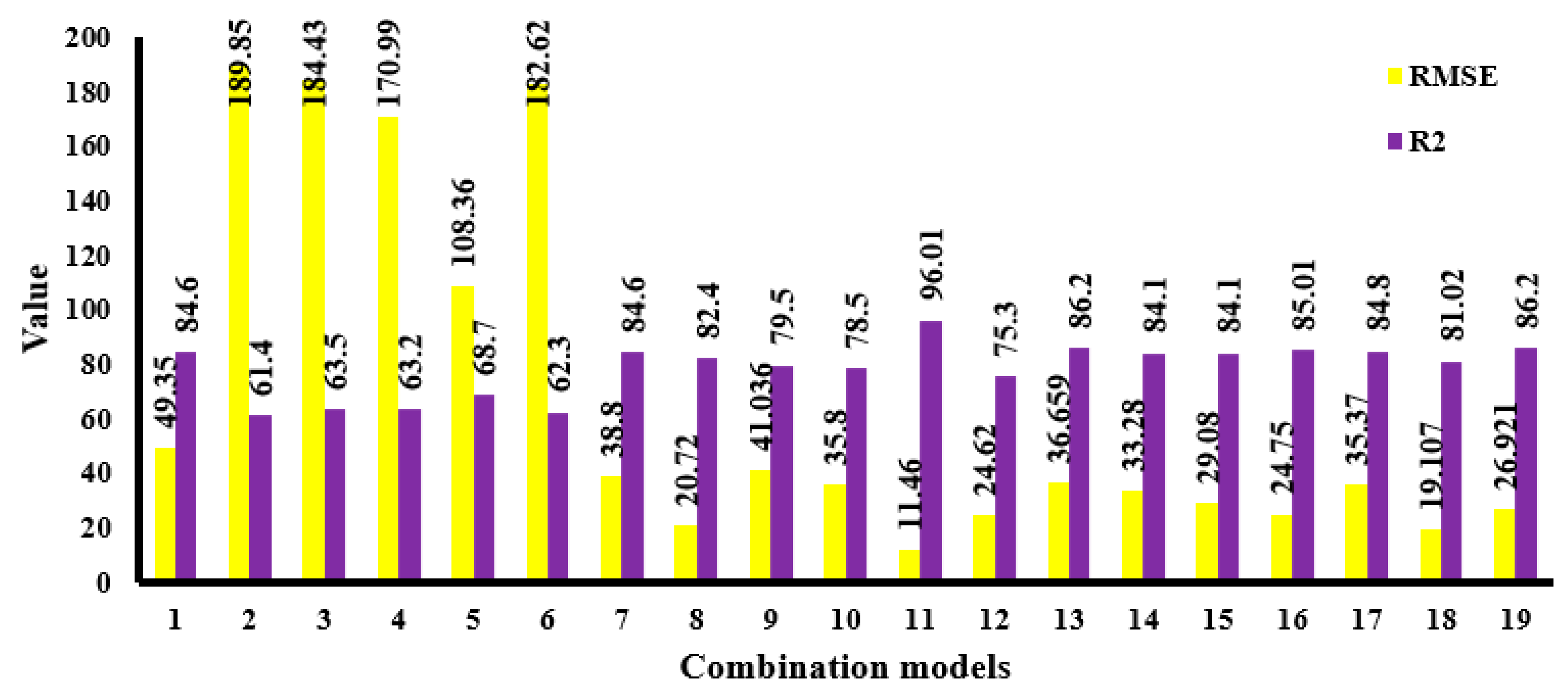
| Num. | Linear Predictive Models | R2 | RMSE |
|---|---|---|---|
| 1 | 84.6 | 49.35 | |
| 2 | 61.4 | 189.85 | |
| 3 | 63.5 | 184.43 | |
| 4 | 63.2 | 170.99 | |
| 5 | 68.7 | 108.36 | |
| 6 | 62.3 | 182.62 | |
| 7 | 84.6 | 38.8 | |
| 8 | 82.4 | 20.72 | |
| 9 | 79.5 | 41.036 | |
| 10 | 78.5 | 35.8 | |
| 11 | 96.01 | 11.46 | |
| 12 | 75.3 | 24.62 | |
| 13 | 86.2 | 36.659 | |
| 14 | 84.1 | 33.28 | |
| 15 | 84.1 | 29.08 | |
| 16 | 85.01 | 24.75 | |
| 17 | 84.8 | 35.37 | |
| 18 | 81.02 | 19.107 | |
| 19 | 86.2 | 26.921 | |
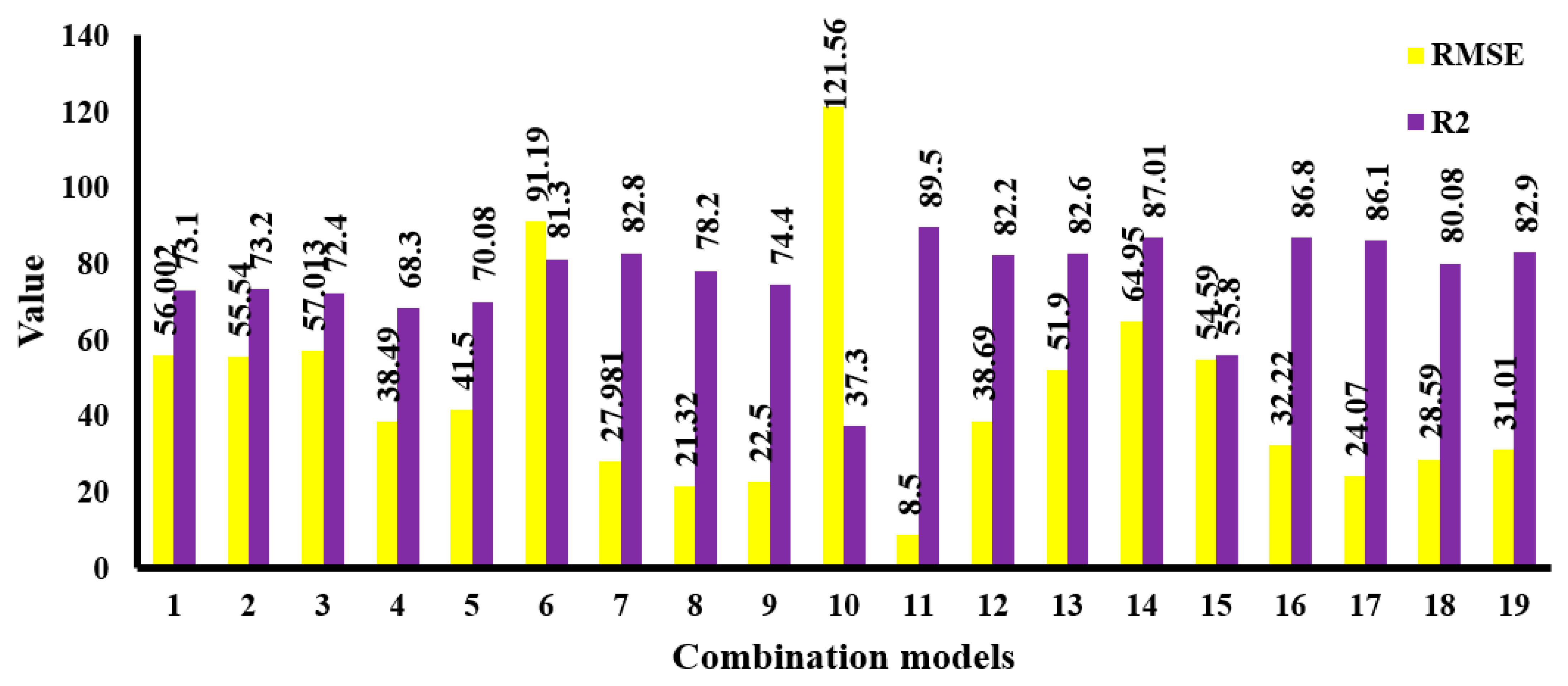
| Num. | Nonlinear Predictive Models | R2 | RMSE |
| 1 | 73.1 | 56.002 | |
| 2 | 73.2 | 55.54 | |
| 3 | 72.4 | 57.013 | |
| 4 | 68.3 | 38.49 | |
| 5 | 70.08 | 41.5 | |
| 6 | 81.3 | 91.19 | |
| 7 | 82.8 | 27.981 | |
| 8 | 78.2 | 21.32 | |
| 9 | 74.4 | 22.5 | |
| 10 | 37.3 | 121.56 | |
| 11 | 89.5 | 8.5 | |
| 12 | 82.2 | 38.69 | |
| 13 | 82.6 | 51.9 | |
| 14 | 87.01 | 64.95 | |
| 15 | 55.8 | 54.59 | |
| 16 | 86.8 | 32.22 | |
| 17 | 86.1 | 24.07 | |
| 18 | 80.08 | 28.59 | |
| 19 | 82.9 | 31.01 |
| Models | 1 | 2 | 3 | 4 | 5 | 6 | 7 | 8 | 9 | 10 |
|---|---|---|---|---|---|---|---|---|---|---|
| Euclidean distance | 0.7 | 9.2 | 0.9 | 9.9 | 0.5 | 0.9 | 0.5 | 0.2 | 0.3 | 9.9 |
| RMSE | 0.1785 | 0.0854 | 0.10743 | 0.0569 | 0.2368 | 0.1051 | 0.2621 | 0.2778 | 0.2621 | 0.0604 |
| R2 | 80.02 | 82.359 | 81.657 | 83.579 | 80.09 | 81.068 | 80.3 | 81.5 | 80.6 | 83.02 |
| Models | 11 | 12 | 13 | 14 | 15 | 16 | 17 | 18 | 19 | |
| Euclidean distance | 9.9 | 9.9 | 9.9 | 9.9 | 9.9 | 9.9 | 9.9 | 9.9 | 9.9 | |
| RMSE | 0.0504 | 0.101 | 0.1252 | 0.05298 | 0.0518 | 0.01476 | 0.247 | 0.1487 | 0.1917 | |
| R2 | 83.489 | 82.746 | 82.964 | 83.529 | 83.419 | 83.961 | 82.513 | 83.725 | 82.197 |
| Populations | 100 | 125 | 150 | 175 | 200 | 225 | 250 | 275 | 300 |
|---|---|---|---|---|---|---|---|---|---|
| RMSE | 0.0622 | 0.0718 | 0.061 | 0.0374 | 0.0529 | 0.0304 | 0.0358 | 0.0664 | 0.0299 |
| R2 | 81.6 | 80.6 | 78.5 | 86.6 | 83.4 | 85.7 | 83.91 | 81.2 | 86.6 |
| Populations | 325 | 350 | 375 | 400 | 425 | 450 | 475 | 500 | |
| RMSE | 0.0155 | 0.0151 | 0.0167 | 0.0949 | 0.0166 | 0.0453 | 0.031 | 0.0396 | |
| R2 | 87.8 | 88.68 | 87.01 | 75.9 | 86.7 | 83.1 | 85.03 | 83.54 |
| Genetic Operators | |
|---|---|
| Chromosome | 30 |
| Genes in each chromosome | 2 |
| Maximum generation | 1000 |
| Gene composition rate | 0.1 |
| Mutation rate | 0.2 |
| Inversion rate | 0.1 |
| Transposition rate | 0.1 |
| Crossover (recombination) (one- and two-point) | 0.8 |
| Fitness function | Root-mean-square deviation |
| Function | Addition (+), Subtraction (−), Multiplication (×), Division (/), Power (x2) |
| Linking function | Addition (+) |
| Num. | GEP Predictive Models | R2 | RMSE |
|---|---|---|---|
| 1 | 91.08 | 36.2308 | |
| 2 | 66.96 | 45.688 | |
| 3 | 84.46 | 39.1689 | |
| 4 | 53.36 | 47.8396 | |
| 5 | 79.77 | 42.7855 | |
| 6 | 89.05 | 37.526 | |
| 7 | 86.12 | 38.1702 | |
| 8 | 58.68 | 47.9883 | |
| 9 | 90.72 | 36.2299 | |
| 10 | 62.94 | 48.2734 | |
| 11 | 64.46 | 48.5888 | |
| 12 | 66.69 | 44.505 | |
| 13 | 71.32 | 44.86 | |
| 14 | 66.15 | 44.084 | |
| 15 | 83.96 | 38.44 | |
| 16 | 87.52 | 37.3659 | |
| 17 | 91.68 | 34.322 | |
| 18 | 73.58 | 42.70 | |
| 19 | 52.65 | 48.601 |
| Parameters | Fuzzy Weight | Deterministic Weight | Rank |
|---|---|---|---|
| Burden (B) | (0.0919, 0.0822, 0.0739) | 0.0827 | 1 |
| S/B | (0.0711, 0.0689, 0.0678) | 0.0693 | 4 |
| Hole diameter (D) | (0.0708, 0.0688, 0.0678) | 0.0691 | 5 |
| Stiffness ratio (H/B) | (0.0676, 0.0675, 0.0676) | 0.0676 | 9 |
| Maximum instantaneous charge (MC) | (0.0676, 0.0680, 0.0681) | 0.0679 | 6 |
| No. of row | (0.0750, 0.0755, 0.0733) | 0.0746 | 3 |
| Powder factor (Pf) | (0.0786, 0.0750, 0.0714) | 0.0750 | 2 |
| Time delay | (0.0490, 0.0557, 0.0605) | 0.0551 | 14 |
| Rock mass rating (RMR) | (0.0593, 0.0598, 0.0623) | 0.060 | 12 |
| B/D ratio | (0.0679, 0.0675, 0.0673) | 0.0675 | 10 |
| Velocity of detonation | (0.0522, 0.0573, 0.0610) | 0.0568 | 13 |
| Blast hole deviation | (0.0471, 0.0513, 0.0575) | 0.0520 | 15 |
| Discontinuities’ orientation to face | (0.0694, 0.0667, 0.0667) | 0.0676 | 8 |
| St/B | (0.0655, 0.0664, 0.0663) | 0.0661 | 11 |
| Bmax | (0.0666, 0.0686, 0.0677) | 0.0676 | 7 |
| B | Value | <1.8 | 1.8–2.04 | 2.04–2.28 | 2.28–2.52 | >2.52 | |
| Ration | 4 | 3 | 2 | 1 | 1 | ||
| S/B | Value | <1.056 | 1.056–1.12 | 1.12–1.16 | 1.16–1.22 | >1.22 | |
| Ration | 0 | 3 | 2 | 1 | 0 | ||
| D | Value | <63 | 63–70 | 70–80 | >80 | ||
| Ration | 4 | 3 | 2 | 1 | |||
| MC | Value | <7 | 7–8.4 | 8.4–10 | 10–12 | >12 | |
| Ration | 4 | 3 | 2 | 1 | 0 | ||
| Pf | Value | <0.226 | 0.226–0.306 | 0.306–0.386 | 0.386–0.466 | >0.466 | |
| Ration | 4 | 3 | 2 | 1 | 0 | ||
| RMR | Value | 0–20 | 20–40 | 40–60 | 60–80 | 80–100 | |
| Ration | 4 | 3 | 2 | 1 | 0 | ||
| B/D | Value | <30.84 | 30.84–35.38 | 35.38–39.91 | >39.91 | ||
| Ration | 3 | 2 | 1 | 0 | |||
| H/B | Value | <2.64 | 2.64–2.96 | 2.96–3.27 | 3.27–3.58 | >3.58 | |
| Ration | 0 | 1 | 2 | 3 | 4 | ||
| St/B | Value | <0.165 | 0.165–0.28 | 0.28–0.39 | 0.39–0.51 | >0.51 | |
| Ration | 0 | 2 | 4 | 3 | 1 | ||
| Velocity of detonation | Value | <3000 | 3000–4000 | 4000–5000 | 5000–6000 | >6000 | |
| Ration | 4 | 3 | 2 | 1 | 0 | ||
| No. of row | Value | <6 | 6–9 | 9–11 | 11–14 | >14 | |
| Ration | 4 | 3 | 2 | 1 | 0 | ||
| Time delay | Value | <2 | 2–4 | 4–6 | 6–7 | 7–9 | >9 |
| Ration | 0 | 1 | 3 | 4 | 2 | 1 | |
| Blast hole deviation | Value | 0–2 | 2–4 | 4–6 | 6–8 | 8–10 | |
| Ration | 4 | 3 | 2 | 1 | 0 | ||
| Discontinuities orientation to face | Value | parallel | vertical | Horizontal | Cross section | ||
| Ration | 4 | 2 | 1 | 3 | |||
| Bmax | Value | 0.5–1 | 1–1.5 | 1.5–2 | 2–2.5 | 2.5–3 | |
| Ration | 4 | 3 | 2 | 1 | 0 |
| Model | Equation | R2 | RMSE |
|---|---|---|---|
| Exponential | 53.40 | 43.27 | |
| Fourier | 80.81 | 36.278 | |
| Gaussian | 87.171 | 34.682 | |
| Polynomial | 62.61 | 41.652 | |
| Power | 40.78 | 46.925 | |
| Sum of sin | 80.04 | 38.263 |
| Flyrock | Blast Number | |||||||||||||
|---|---|---|---|---|---|---|---|---|---|---|---|---|---|---|
| 1 | 2 | 3 | 4 | 5 | 6 | 7 | 8 | 9 | 10 | 11 | 12 | 13 | 14 | |
| Empirical Equation (1) | 540.8 | 540.8 | 540.8 | 540.8 | 478.92 | 540.8 | 478.92 | 478.92 | 540.8 | 540.8 | 478.92 | 540.8 | 540.8 | 540.8 |
| Empirical Equation (2) | 68.907 | 68.907 | 68.907 | 68.907 | 132.68 | 103.36 | 79.613 | 88.45 | 68.907 | 68.907 | 132.68 | 86.134 | 120.588 | 86.134 |
| Linear regression | 214.03 | 152.35 | 201.6 | 153.25 | 127.71 | 150.08 | 104.58 | 114.88 | 136.73 | 184.72 | 162.81 | 175.63 | 249.75 | 164.28 |
| Nonlinear regression | 196.14 | 150.61 | 208.69 | 151.59 | 129.4 | 142.232 | 120.12 | 111.35 | 137.36 | 183.4 | 148.83 | 175.12 | 142.94 | 168.31 |
| Gaussian | 370.6 | 519.62 | 146.66 | 169.86 | 132.65 | 134.65 | 120.7 | 119.54 | 100.45 | 107.7 | 189.657 | 189.27 | 215.65 | - |
| GRNN | 211.36 | 152.96 | 221.03 | 140.26 | 122.85 | 124.87 | 124.35 | 113.71 | 142.72 | 198.77 | 163.67 | 160.46 | 157.17 | 169.57 |
| GA-GRNN | 254.58 | 162.78 | 214.38 | 148.31 | 138.33 | 129.19 | 134.28 | 121.93 | 141.56 | 192.79 | 143.92 | 146.58 | 137.26 | 165.60 |
| GEP | 253.58 | 161.51 | 213.53 | 150.77 | 140.91 | 132.19 | 130.27 | 119.68 | 138.01 | 190.44 | 138.6 | 151.73 | 143.51 | 158.36 |
| Flyrock | Blast Number | |||||||||||||
| 15 | 16 | 17 | 18 | 19 | 20 | 21 | 22 | 23 | 24 | 25 | 26 | 27 | 28 | |
| Empirical Equation (1) | 478.92 | 540.8 | 540.8 | 478.92 | 540.8 | 540.8 | 478.92 | 540.8 | 540.8 | 540.8 | 478.92 | 540.8 | 540.8 | 478.92 |
| Empirical Equation (2) | 110.57 | 68.907 | 103.36 | 88.45 | 68.907 | 68.907 | 154.80 | 68.907 | 86.134 | 103.36 | 79.613 | 68.907 | 68.907 | 88.459 |
| Linear regression | 201.30 | 145.78 | 235.59 | 195.40 | 151.512 | 146.25 | 283.85 | 201.6 | 257.75 | 236.141 | 161.65 | 153.258 | 153.258 | 201.6 |
| Nonlinear regression | 210.48 | 145.80 | 233.75 | 185.63 | 153.25 | 146.35 | 246.78 | 209.71 | 247.74 | 224.63 | 160.07 | 151.59 | 151.591 | 211.67 |
| Gaussian | 194.65 | 176.28 | 255.63 | 130.85 | 149.68 | 139.46 | 176.85 | 293.76 | 146.37 | 115.78 | 194.64 | 154.17 | 189.98 | 248.18 |
| GRNN | 196.02 | 161.13 | 214.50 | 174.31 | 136.002 | 136.108 | 237.56 | 201.5 | 263.95 | 199.28 | 130.74 | 117.02 | 115.93 | 191.32 |
| GA-GRNN | 144.77 | 158.52 | 137.31 | 161.30 | 156.80 | 163.121 | 139.79 | 212.29 | 221.37 | 142.11 | 116.23 | 148.64 | 151.75 | 211.27 |
| GEP | 151.36 | 159.52 | 143.57 | 157.71 | 151.55 | 160.75 | 145.05 | 213.53 | 211.12 | 143.06 | 116 | 150.77 | 150.771 | 213.53 |
| Out Put | Function | MAPE | VAF | R2 | RMSE |
|---|---|---|---|---|---|
| Flyrock | Empirical Equation (1) | 232.23 | 21.225 | 6.04 | 356.113 |
| Empirical Equation (2) | 44.875 | −12.707 | 27.01 | 96.755 | |
| Linear regression | 19.908 | 45.009 | 60.88 | 43.701 | |
| Nonlinear regression | 17.802 | 59.015 | 64.54 | 38.938 | |
| Gaussian | - | - | 48.08 | 31.415 | |
| GRNN | 13.806 | 80.739 | 82.83 | 32.1809 | |
| GA-GRNN | 14.258 | 87.604 | 87.74 | 30.753 | |
| GEP | 14.451 | 86.528 | 86.8 | 31.166 |
Disclaimer/Publisher’s Note: The statements, opinions and data contained in all publications are solely those of the individual author(s) and contributor(s) and not of MDPI and/or the editor(s). MDPI and/or the editor(s) disclaim responsibility for any injury to people or property resulting from any ideas, methods, instructions or products referred to in the content. |
© 2023 by the authors. Licensee MDPI, Basel, Switzerland. This article is an open access article distributed under the terms and conditions of the Creative Commons Attribution (CC BY) license (https://creativecommons.org/licenses/by/4.0/).
Share and Cite
Babaeian, M.; Sereshki, F.; Ataei, M.; Nehring, M.; Mohammadi, S. Application of Soft Computing, Statistical and Multi-Criteria Decision-Making Methods to Develop a Predictive Equation for Prediction of Flyrock Distance in Open-Pit Mining. Mining 2023, 3, 304-333. https://doi.org/10.3390/mining3020019
Babaeian M, Sereshki F, Ataei M, Nehring M, Mohammadi S. Application of Soft Computing, Statistical and Multi-Criteria Decision-Making Methods to Develop a Predictive Equation for Prediction of Flyrock Distance in Open-Pit Mining. Mining. 2023; 3(2):304-333. https://doi.org/10.3390/mining3020019
Chicago/Turabian StyleBabaeian, Mohammad, Farhang Sereshki, Mohammad Ataei, Micah Nehring, and Sadjad Mohammadi. 2023. "Application of Soft Computing, Statistical and Multi-Criteria Decision-Making Methods to Develop a Predictive Equation for Prediction of Flyrock Distance in Open-Pit Mining" Mining 3, no. 2: 304-333. https://doi.org/10.3390/mining3020019
APA StyleBabaeian, M., Sereshki, F., Ataei, M., Nehring, M., & Mohammadi, S. (2023). Application of Soft Computing, Statistical and Multi-Criteria Decision-Making Methods to Develop a Predictive Equation for Prediction of Flyrock Distance in Open-Pit Mining. Mining, 3(2), 304-333. https://doi.org/10.3390/mining3020019