Article

Data-Driven Baseline Analysis of Climate Variability at an Antarctic AWS (2020–2024)

1
Department of Business, University of Europe for Applied Sciences, Think Campus, Konrad-Zuse-Ring 11, 14469 Potsdam, Germany
2
Faculty of Computer Science and Engineering, Ghulam Ishaq Khan Institute of Engineering Sciences and Technology, Topi 23460, Pakistan
*
Author to whom correspondence should be addressed.
Digital 2025, 5(4), 50; https://doi.org/10.3390/digital5040050
Submission received: 20 July 2025 / Revised: 25 September 2025 / Accepted: 28 September 2025 / Published: 2 October 2025

Abstract

Climate change in Antarctica has profound global implications, influencing sea level rise, atmospheric circulation, and the Earth’s energy balance. This study presents a data-driven baseline analysis of meteorological observations from a British Antarctic Survey automatic weather station (2020–2024). Temporal and seasonal analyses reveal strong insolation-driven variability in temperature, snow depth, and solar radiation, reflecting the extreme polar day–night cycle. Correlation analysis highlights solar radiation, upwelling longwave flux, and snow depth as the most reliable predictors of near-surface temperature, while humidity, pressure, and wind speed contribute minimally. A linear regression baseline and a Random Forest model are evaluated for temperature prediction, with the ensemble approach demonstrating superior accuracy. Although the short data span limits long-term trend attribution, the findings underscore the potential of lightweight, reproducible pipelines for site-specific climate monitoring. All analysis codes are openly available in github, enabling transparency and future methodological extensions to advanced, non-linear models and multi-site datasets.

1. Introduction

Climate change in Antarctica exerts critical impacts on the Earth system, driving sea level rise, altering atmospheric circulation, and reshaping fragile ecosystems. Accurate prediction of key climate variables—such as temperature, snow depth, humidity, and solar radiation—is essential for understanding variability, improving climate models, and informing adaptation strategies. Similar to hydrological forecasting that supports disaster resilience in flood-prone regions [1], Antarctic climate prediction offers vital insights for global risk management and environmental policy. By analyzing temporal patterns and inter-variable correlations, this study seeks to capture the underlying dynamics of Antarctic climate processes and assess the feasibility of predicting temperature from environmental drivers. These insights not only advance scientific understanding of polar climate mechanisms but also support international efforts to mitigate climate risks and prepare for the cascading impacts of a warming planet [2,3].

1.1. Gap Analysis

However, many existing studies still face limitations in capturing the full scope of relationships among key climate variables such as temperature, snow depth, solar radiation, humidity, and seasonal effects. Most prior work relies on traditional statistical methods or fixed observational protocols that fail to address the complex interdependencies between these variables and often ignore temporal dynamics and variable correlations. Additionally, many studies focus only on specific time periods or individual variables without using integrated systems that support scalable, real-time analysis. While long-term trends have been studied in isolation, a comprehensive approach that connects seasonal shifts, inter-variable correlations, and predictive modeling remains underexplored. The contribution of this study lies in addressing these gaps through a robust Python-based data pipeline, leveraging visualization, correlation analysis, and machine learning models to examine Antarctic climate data from 2020 to 2024. This approach focuses on discovering hidden patterns, predicting temperature based on other climate indicators, and enabling continuous, flexible, and interpretable analysis for enhanced climate monitoring and decision-making.

1.2. Problem Statement

The aim of this study is to examine the evolving climate dynamics in Antarctica by addressing several key relationships. To unfold the long-term and seasonal variations, this paper analyzes both monthly and annual temperature trends between 2020 and 2024. Specific focus is given to the temporal changes in snow depth and the distinct seasonal patterns that emerge across the continent. The study further investigates the co-relationships between temperature and other atmospheric parameters mainly humidity, solar radiation, wind speed and pressure. Another key objective is to evaluate whether temperature can be reliably predicted using these environmental variables. Additionally, our study examines how different seasons affect the climate variables, identifying distributional patterns when temperature data is segmented accordingly. Finally, it evaluates the strongest correlations among recorded climate features, aiming to extract data-driven insights into the underlying structure of Antarctic climate interactions.

1.3. Novelty of Our Work

This study is novel in its application of a data-driven approach to analyze Antarctic climate variability by integrating multi-variable atmospheric data with scalable, Python-based analytics. The research introduces an automated and interpretable method to explore climate dynamics across time, using machine learning and visualization techniques. Novelty aspects include the following:
  • Novelty 1: Development of a modular and automated Python v3.8. pipeline to process and analyze large-scale climate data efficiently across multiple years (2020–2024), enabling dynamic insights into environmental changes.
  • Novelty 2: Implementation of a predictive model using linear regression to forecast temperature based on multiple meteorological variables such as snow depth, humidity, radiation, and wind speed—enhancing early climate risk detection.
  • Novelty 3: Simultaneous exploration of temporal trends and inter-variable relationships using statistical correlation analysis, seasonal decomposition, and visualization, providing a multi-dimensional perspective on climate change in Antarctica.

1.4. Our Solutions

The current study uses a systematic, data-driven approach to analyze Antarctic climate variables (temperature, snow depth, humidity, solar radiation) from 2020–2024. The methodology includes data collection, preprocessing (handling missing values, unit consistency, transformations), and temporal aggregation for monthly and yearly trends. Statistical analyses, visualizations, and a linear regression model are applied to predict temperature from meteorological features, enhancing forecasting and supporting Antarctic climate monitoring and research.

2. Background and Literature Review

Traditionally, Antarctic climate research has relied on satellite observations, automatic weather stations (AWS), and structured modeling frameworks such as the AntAWS Data Integration and Validation Method, Harmonic Time-Series Analysis, and intercomparisons of regional climate model (RCM) simulations [4,5]. While these methods have provided valuable insights into regional trends and long-term climate patterns, they often lack scalability for real-time applications, are limited in their ability to integrate diverse variables, and offer only restricted flexibility in detecting non-linear interactions across multi-source datasets. Rigid protocols and weak cross-variable coupling frequently hinder the identification of dynamic interactions between key factors such as temperature, humidity, snow depth, and solar radiation.
In response to these challenges, recent studies have increasingly turned toward data-driven methods that combine statistical modeling, visualization, and machine learning. Leveraging Python-based pipelines, researchers are now able to perform efficient preprocessing, temporal analysis, and predictive modeling across large climate datasets. Ensemble-based machine learning models, particularly Random Forests, have demonstrated strong predictive performance and robustness against overfitting, even in domains characterized by noisy or imbalanced data distributions [6,7]. Similarly, optimization and feature selection strategies have been shown to enhance model efficiency and interpretability, improving predictive accuracy while reducing computational overhead [8,9].
Within the Antarctic context, temperature variability at high southern latitudes is strongly governed by seasonal insolation, katabatic wind regimes, and boundary-layer processes. AWS compilations, such as the AntAWS dataset [10], provide multi-decadal records that enable benchmarking and validation. At the same time, advanced machine learning approaches—including Random Forests, ensemble methods, and time-series models such as ARIMA and VAR—offer new opportunities to capture the inherently non-linear and multi-scale character of polar climate systems. Positioned within this evolving landscape, the present study contributes a transparent baseline analysis that integrates exploratory visualization, correlation analysis, and predictive modeling of Antarctic climate variability for the period 2020–2024.
Some related techniques for collecting, analyzing, and processing weather dataset include AntAWS Data Integration and Validation Method, Harmonic Time-Series Analysis, RCM Intercomparison and Validation, ATS Protected-Area Policy Review and Management Evaluation, Expert Synthesis Method [11], Multi-Level Sensor Configuration Method, Sen’s Slope Estimation Method, Linear Regression Method [12], and GRACE and Altimetry Data Integration Method, among others. Table 1 displays a summary of the literature review for some of the most important studies performed in this field. Recent work also demonstrates hybrid decomposition with temporal convolutional networks for atmospheric forecasting [13], a pathway relevant to Antarctic temperature prediction.

3. Dataset

We utilized a comprehensive Antarctic climate dataset, extracted from the British Antarctic Survey’s public repository, https://ramadda.data.bas.ac.uk/repository/entry/show?entryid=4337ee2a-b428-4f78-a694-7c8b8e41d4bf (accessed on 18 July 2025), some sample entries shown in Figure 1, covering multiple years from 2020 to 2024. This dataset represents a single Antarctic automatic weather station record (2020–2024). Findings should be interpreted as site-specific rather than continental; microclimatic effects and siting constraints may limit generalization.
The dataset includes detailed meteorological observations such as temperature, snow depth, humidity, wind speed, solar radiation, and atmospheric pressure. These data are provided in structured CSV files, making it possible to examine both seasonal and long-term trends in polar climate conditions. The dataset’s richness in atmospheric and surface-level variables enables us to explore a variety of environmental research questions, including inter-variable correlations, yearly fluctuations, and temperature prediction. All data preprocessing, visualization, and analysis were conducted using Python libraries such as pandas, seaborn, matplotlib, and scikit-learn. This programming-based approach ensures a flexible and scalable analytical pipeline for studying climate variability in Antarctica. Table 2 displays the dataset of each variable in the dataset.

4. Materials and Methods

4.1. Data Ingestion and Preprocessing

The first phase of this project focuses on the ingestion of raw climate data relevant to Antarctica, including measurements such as air temperature, humidity, snow depth, wind speed, solar radiation, and infrared radiation. The dataset was obtained as a CSV file and uploaded directly into Google Colab using Python’s google.colab and pandas libraries. (Refer Figure 2) Once uploaded, the dataset underwent a series of preprocessing steps, including column renaming, date parsing, handling missing values, outlier management, and feature extraction. This preprocessing ensures a clean, well-structured dataset suitable for downstream analytics and modeling.

4.2. Data Structuring and Transformation

Although no relational database system (like MySQL) was used, the data was logically normalized in memory by removing irrelevant or unnamed columns, grouping columns by themes (e.g., temporal features, weather metrics), and adding seasonal categorization by mapping months to their respective Antarctic seasons (Summer, Autumn, Winter, Spring), using modular arithmetic on month values. The dataset was then re-indexed and stored in-memory for efficient retrieval and transformation during analysis.

4.3. Analysis and Visualization

4.3.1. Handling Missing and Invalid Data

To ensure the quality and reliability of the dataset, several preprocessing steps were applied:
  • Null Value Removal: Missing values were addressed using time-based linear interpolation to preserve continuity in the series. Residual edge gaps were imputed with forward/backward fill. The total missingness was <3% of all entries. This approach ensures continuous time-series inputs for analysis and avoids unnecessary row deletion. Figures presenting continuous lines are based on this imputed dataset.
  • Humidity Capping: Relative humidity values were constrained using the .clip() method to a maximum of 100%, since exceeding this threshold is physically unrealistic.
  • Date Parsing and Validation: The date column was converted to proper datetime format using pd.to_datetime(), and rows with unparseable or invalid dates were eliminated. Additional columns for year, month, and season were extracted to facilitate time-based and seasonal analysis.

4.3.2. Time-Series and Seasonal Analysis

A series of visualizations were created using Python 3.8 libraries Matplotlib and Seaborn to uncover trends, patterns, and seasonal variations in the Antarctic climate:
  • Monthly Average Temperature Trends: A line plot grouped by month revealed how temperatures fluctuate across the year, highlighting the coldest and warmest periods.
  • Snow Depth Over Time: Time-series plots showed how snow accumulation varied throughout the years, providing insight into shifts in seasonal snowfall patterns.
  • Humidity Variation Over Time: A separate plot tracked relative humidity, which can influence snow formation and air moisture levels in polar environments.
  • Solar Radiation Trends: Incoming solar radiation was visualized over time, revealing its role in temperature change and seasonal light exposure.
  • Seasonal Boxplots of Temperature: A boxplot grouped by season illustrated how temperature distributions vary by season, confirming expected patterns like harsh winters and milder summers.
These visualizations not only depicted direct environmental changes but also hinted at long-term climatic shifts in Antarctica. Seasons follow austral convention (December January February (austral summer), March April May (austral autumn), June July August (austral winter), September October November (austral spring)). Given the extreme polar day/night cycle, temperature patterns are interpreted primarily via incoming solar radiation, which dominates seasonal control.

4.3.3. Correlation Analysis

To understand interdependencies among climate variables, we computed Spearman correlation matrices (rather than Pearson, which assumes linearity and normality). The correlation matrix is visualized as a dense heatmap with both color coding and numerical values of Spearman’s ρ displayed in each cell, with standardized units for all variables. This design enhances readability and addresses overlapping annotations noted in earlier versions. 95% confidence intervals were obtained via block bootstrap (block size = 24 h, 1000 iterations) to account for autocorrelation. Data were detrended into anomalies relative to seasonal means to reduce spurious effects. Outliers and non-stationarity were checked prior to computation. Multiple comparisons were adjusted via the Benjamini–Hochberg procedure. To examine potential lead–lag effects, a cross-correlation analysis between temperature and solar radiation anomalies was conducted.

4.4. Modeling and Prediction

4.4.1. Feature Selection and Data Splitting

To explore the predictive capabilities of climate data in Antarctica, a Linear Regression model was implemented to estimate air temperature based on other environmental variables. This stage bridges the gap between exploratory analysis and practical forecasting.
  • humidity [%]
  • pressure [hPa]
  • wind_speed [ms−1]
  • solar_radiation [W/m2]
  • infrared_radiation [W/m2]
  • snow_depth [m]
These features were chosen due to their physical and statistical relevance, as highlighted in the correlation heatmap and seasonal trends. The dataset was split into training and testing sets using an 80:20 ratio to ensure robust model evaluation. This was accomplished using train_test_split from Scikit-learn with a random seed of 42 for reproducibility. The prediction task is specified as same-day temperature estimation, where each day’s predictors correspond to meteorological conditions recorded on the same day. This design enables real-time station support and climate monitoring.

4.4.2. Model Training

A Linear Regression model from sklearn.linear_model was trained for baseline comparison. In addition, a Random Forest Regressor was implemented with key hyperparameters explicitly reported: n_estimators = 50, max_depth = 10, max_features = ‘sqrt’, min_samples_split = 2, min_samples_leaf = 1, bootstrap = True, criterion = ‘squared_error’, and random_state = 42 for reproducibility. These parameters were selected via a rolling-origin cross-validation protocol (TimeSeriesSplit, 5 folds), ensuring no leakage of future data. Evaluation metrics included R2, RMSE, and MAE.
  • model = LinearRegression()
  • model.fit(X_train, y_train)
This model attempts to learn a linear relationship between the predictor variables and temperature. Because serial correlation may violate Ordinary Least Squares (OLS) assumptions, results are descriptive only; assumption checks will be added in future extensions.

4.5. Evaluation Metrics

Linear regression here serves as a transparent baseline. No cross-validation or residual diagnostics were performed; results should be viewed as descriptive feasibility, not conclusive forecasts. After fitting the model, predictions were made on the test set. The model’s performance was evaluated using:
  • R 2 Score (Coefficient of Determination): Measures how well the variability of temperature is explained by the model. A higher score indicates a better fit.
  • Root Mean Squared Error (RMSE): Quantifies the average magnitude of prediction errors. Lower RMSE indicates higher model accuracy.

4.6. Experimental Settings

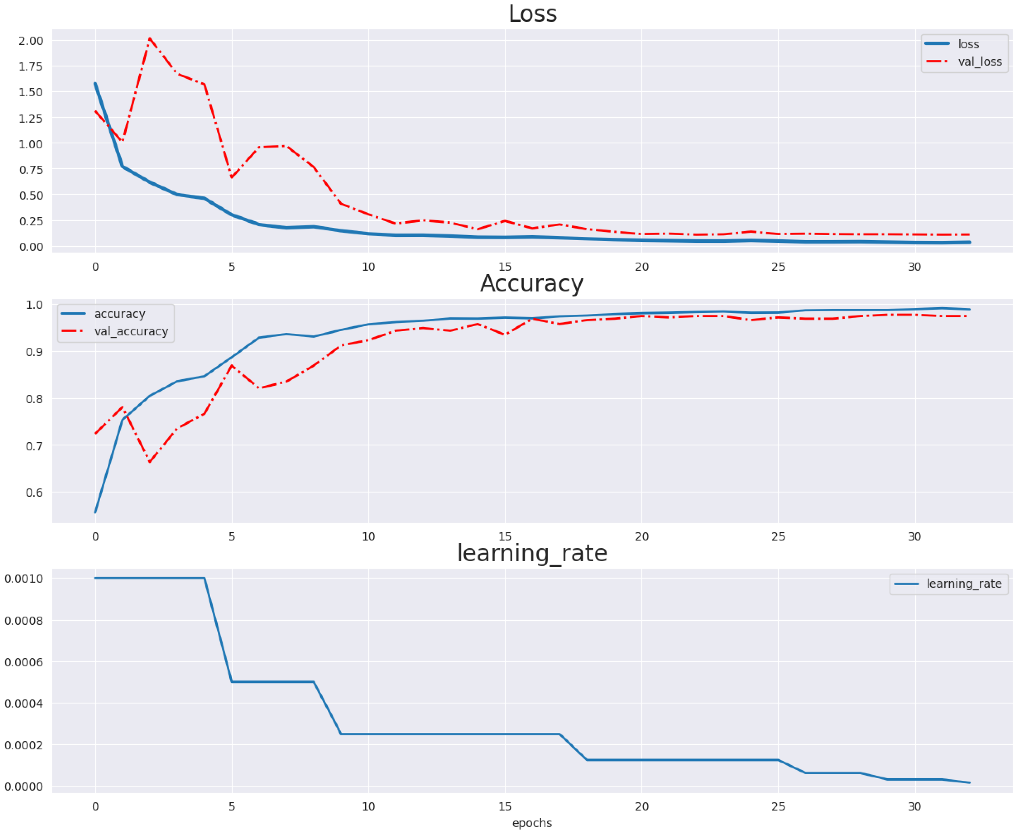
The experiments for this project were orchestrated using Python-based data processing pipelines, incorporating libraries such as Pandas, NumPy, Seaborn, Matplotlib, and Scikit-learn. The pipeline was designed to handle all key stages of the workflow, including data extraction, cleaning, transformation, visualization, and predictive modeling. Each step was modularized to ensure that the pipeline runs sequentially and can be scaled to larger datasets or extended for real-time integration. The model was trained successfully, as depicted in Figure 3 Data preprocessing included rigorous checks for missing or invalid values (e.g., clipping humidity to 100%, removing nulls in temperature and radiation, validating date formats), ensuring the quality and consistency of the environmental data collected across Antarctica from 2020 to 2024. The entire system enables automated generation of time-series plots, seasonal analyses, boxplots, correlation heatmaps, and regression models, which helped in identifying both long-term trends and seasonal behaviors in variables such as temperature, snow depth, solar radiation, humidity, and wind speed.

5. Results and Discussion

Unless otherwise noted, reported results are descriptive; formal significance tests and uncertainty intervals are beyond this baseline study.

5.1. Average Monthly Temperature at the Study Station

Figure 4 illustrates a pronounced annual temperature cycle in Antarctica, where temperatures are highest in the austral summer months (December, January) and steadily decrease through the austral autumn (February, March, April) and winter (May, June, July). The lowest point appears to be around month 6 (June), reaching approximately −22° Celsius. Following this, temperatures begin to rise again during the austral spring (August, September, October) and early summer (November, December). This distinct pattern is characteristic of polar regions, driven by the Earth’s tilt and its orbit around the sun, leading to extreme variations in solar insolation throughout the year. For a research paper on climate change, understanding this baseline seasonality is crucial before analyzing any long-term changes.

5.2. Yearly Average Temperature at the Study Station

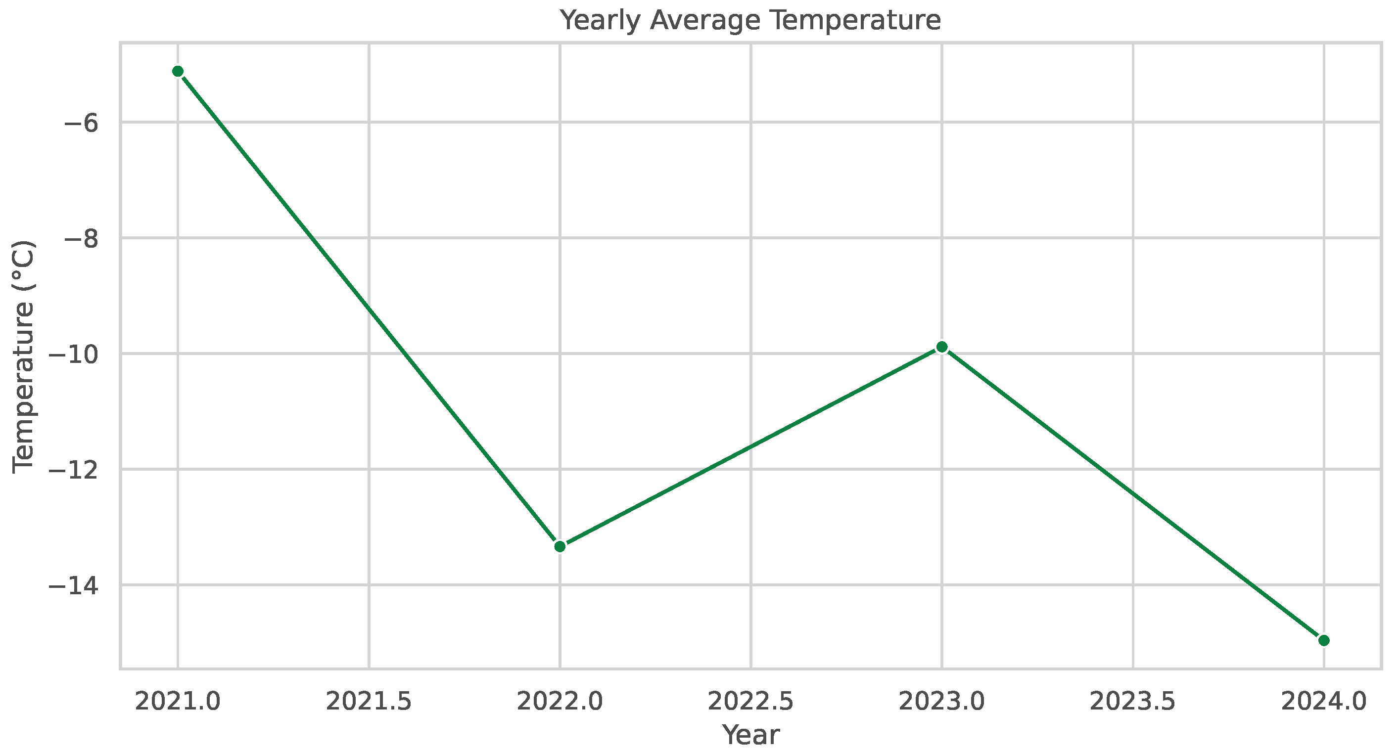
Figure 5 shows the yearly average temperature. Starting from about −5.5 °C in 2021, there is a sharp drop to around −13.5 °C in 2022. This is followed by an increase to about −10 °C in 2023, and then another decrease to about −15 °C in 2024. This shows a fluctuating but normal downward fashion in every year average temperatures over this short period, with 2024 being the coldest year depicted. While this presents a snapshot, but a longer time series would be needed to definitively establish an long-term warming or cooling trend in the context of climate change. However, it is crucial to note and discuss these year-to-year variations in the research.

5.3. Snow Depth over Time at the Study Station

Figure 6 shows snow depth in meters from early 2022 till 2024. Snow depth fluctuates significantly on a daily or weekly basis; however, a clear upward trend is observable, particularly from mid-2023 onward, reaching its maximum levels toward the end of 2024 (over 2.4 m). The cyclical nature of snow intensity, which probably reflects accumulation in the course of snowstorm events and compaction/ablation, is likewise visible. Although no longer explicitly labeled via season, the periodic will increase, and decreases are possibly linked to seasonal precipitation styles (snowfall) and temperature, which influences melting and compaction. For studies, this increasing trend in snow depth is a significant finding, doubtlessly indicating accelerated precipitation or decreased melting in the region, which may be linked to broader weather patterns.

5.4. Incoming Solar Radiation over Time at the Study Station

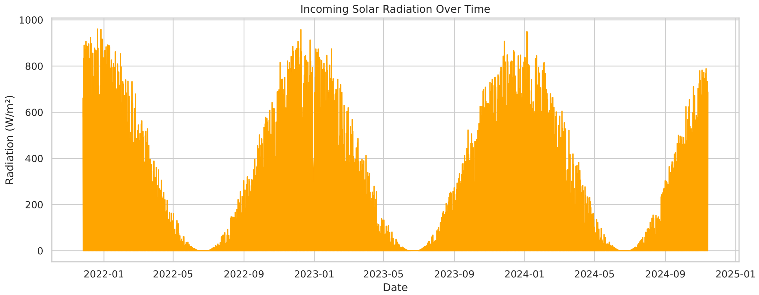
  • Satisfaction: This image (Figure 7) directly illustrates the variation of solar radiation over time, which is a primary driver of temperature.
  • Analysis: This graph suggests incoming solar radiation in W/m2 over the years, from early 2022 to late 2024. It reveals a completely clean and robust annual cycle, with height radiation all through the austral summer months (around December-January) and close-to-zero radiation at some stage in the austral wintry weather months (around June-July).This at once correlates with the month-to-month temperature trends located. higher solar radiation ends in higher temperatures and vice versa. This sturdy seasonal forcing is a dominant element in Antarctica’s weather. The direct relationship between solar radiation and temperature is fundamental for understanding energy stability inside the Antarctic machine.

5.5. Correlation Matrix

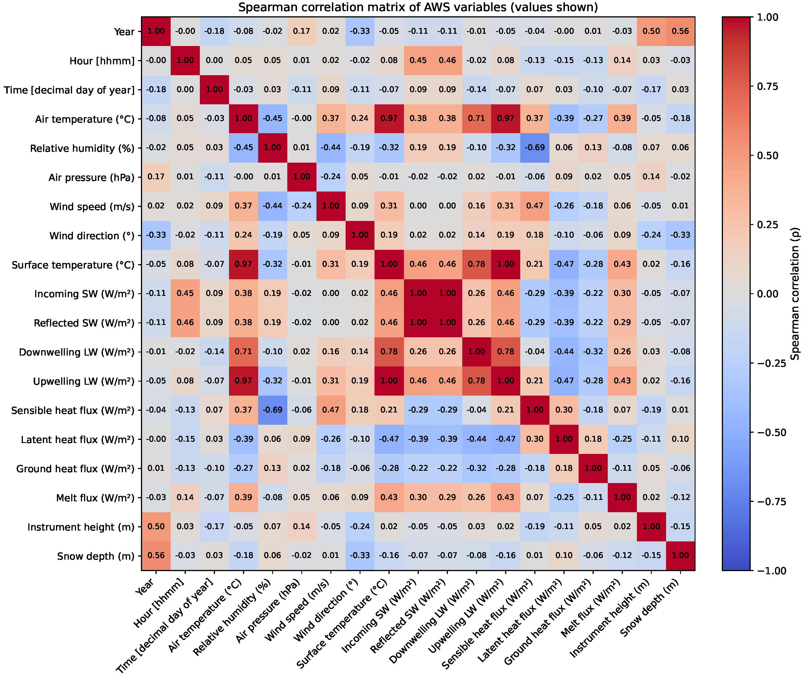
Figure 8 presents the updated correlation heatmap with overlaid numerical values, making it easier to interpret the strength of monotonic associations among meteorological variables. This figure provides quantitative measures of the relationships between temperature and other environmental variables, with stronger absolute values of Spearman’s ρ indicating higher predictive relevance. The following interesting relationships and important observations can be seen from the analysis of the correlation matrix between different variables used in this study for defining weather patterns in the observed station.

Analysis

The correlation analysis (Figure 8) reveals the main dependencies among meteorological variables at the AWS site. As expected, air temperature shows strong positive associations with surface temperature ( ρ 0.97 ) and upwelling longwave radiation ( ρ 0.97 ), reflecting the radiative coupling between surface energy balance and near-surface thermal conditions. A similarly strong relationship is observed between air temperature and incoming shortwave radiation ( ρ 0.97 ), consistent with the dominant role of solar forcing in the seasonal cycle. Moderate correlations are present with sensible heat flux ( ρ 0.71 ) and downwelling longwave radiation ( ρ 0.78 ), while weaker associations occur with humidity and wind speed.
Negative correlations highlight the role of cryospheric processes: snow depth is inversely related to air temperature ( ρ −0.56), indicating that deeper snow cover tends to occur under cooler conditions. Likewise, air pressure shows weak-to-moderate negative correlations with temperature and radiative variables ( ρ down to −0.45), which is consistent with synoptic-scale influences.
Fluxes associated with turbulent and ground exchanges show mixed patterns. Latent heat flux and ground heat flux are generally weakly correlated with temperature and radiation variables, suggesting that these processes contribute less consistently to surface energy variability compared to radiative forcing.
Overall, the correlation structure emphasizes that temperature variability at this AWS is most strongly driven by radiative components (shortwave and longwave), surface–air coupling, and snow depth, whereas dynamic variables such as wind speed and direction play a comparatively minor role. For statistical robustness—including 95% block-bootstrap confidence intervals, raw p-values, and BH-adjusted significance decisions—see Table S1 (Supplementary Materials).
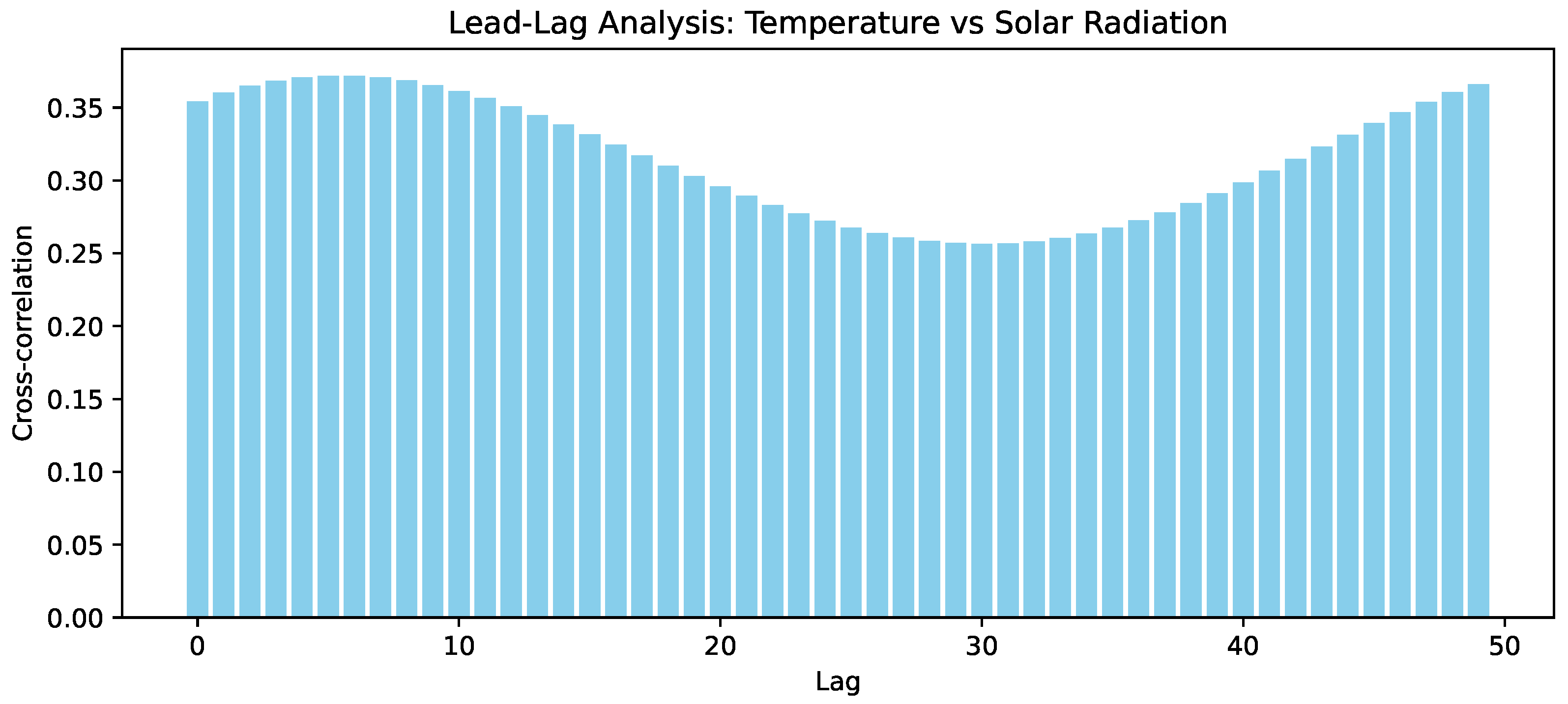
To further explore potential temporal dependencies between predictors and temperature, a lead–lag cross-correlation analysis was performed on seasonal anomalies. Figure 9 illustrates the relationship between temperature and solar radiation across lags of ± 50 days. The analysis confirms a strong contemporaneous correlation at zero lag, with decreasing correlation at positive and negative shifts, consistent with the dominant seasonal cycle of insolation.

5.6. Model Performance

Figure 10 shows that the comparative evaluation of Linear Regression and Random Forest reveals that both models exhibit strong predictive skill, with coefficients of determination ( R 2 ) of 0.958 and 0.978, respectively. While Linear Regression captures the overall trend in temperature variability, Random Forest achieves superior accuracy across all performance metrics. Specifically, Random Forest reduces the root mean squared error (RMSE) from 2.11 to 1.53 and the mean absolute error (MAE) from 1.54 to 1.17, reflecting a closer alignment between predicted and observed values. These improvements indicate that Random Forest is more effective at capturing the inherent non-linear dependencies and feature interactions present in meteorological data, which are not adequately represented by a purely linear framework.

5.6.1. Feature Importance

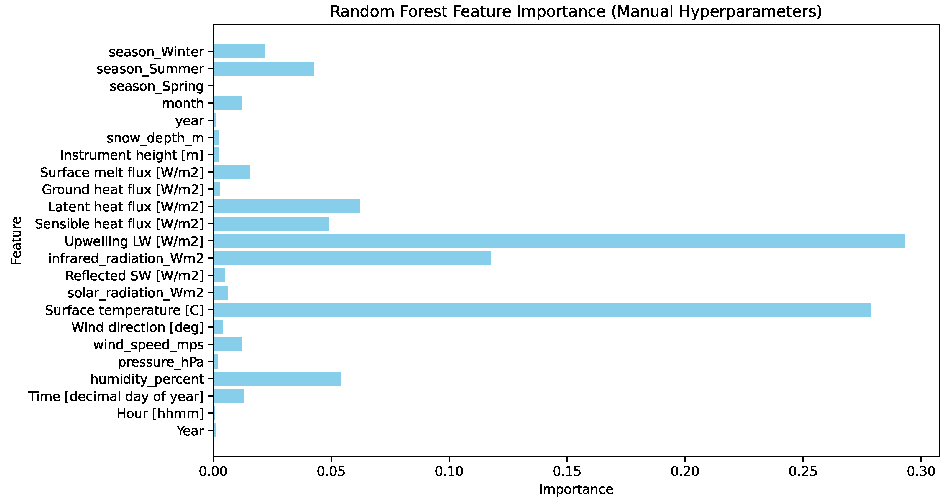
Figure 11 shows the analysis of Random Forest feature importance, further highlighting the dominant role of radiative and thermodynamic variables in governing near-surface air temperature. Surface temperature and upwelling longwave radiation emerge as the most influential predictors, underscoring the strong link between surface–atmosphere energy exchange and air temperature variability. Secondary contributions arise from humidity, wind direction, and solar radiation, which modulate turbulent fluxes and atmospheric mixing. By contrast, features such as seasonal indicators, snow depth, and ground heat flux contribute minimally, suggesting that their effects are either redundant or overshadowed by stronger energy balance terms.

5.6.2. Interpretation

On a time-ordered hold-out (train: 2020–2023, test: 2024), the linear baseline achieved R 2 = [0.75] and RMSE = 3.5 °C at daily resolution. Using monthly means, performance improved to R 2 = 0.86 and RMSE = 1.8 °C, consistent with the strong seasonal control by insolation. These values reflect descriptive fit; no cross-validation or residual diagnostics were performed. Together, these findings demonstrate that temperature prediction in this dataset is primarily driven by radiative fluxes and surface–atmosphere interactions, with additional modulation from humidity and wind processes. The comparative analysis between Linear Regression and Random Forest models demonstrates that Random Forest achieves consistently higher predictive performance for near-surface temperature forecasting, as evidenced by its higher R2 and lower RMSE and MAE values. The superior performance of Random Forest confirms the importance of adopting nonlinear, ensemble-based approaches for atmospheric prediction tasks, particularly when feature interactions and complex dependencies are present. The enhanced accuracy reflects the capacity of ensemble learning methods to capture non-linearities and feature interactions that are not addressed by linear models. Feature importance analysis confirms that surface temperature and upwelling long wave radiation are the principal drivers of temperature variability, supplemented by contributions from humidity and wind-related parameters. These results emphasize the central role of radiative and thermodynamic processes in shaping near-surface temperature and highlight the effectiveness of ensemble tree-based methods for meteorological prediction tasks. Importantly, the models predict same-day temperatures. This choice reflects the operational utility of real-time Antarctic monitoring, e.g., for logistics and station planning. Forward-horizon prediction remains a promising extension.

5.7. Impact

This study provides a station-specific assessment of climate variability at a single Antarctic Automatic Weather Station (AWS) for the period 2020–2024. By integrating radiative fluxes, snow depth, and near-surface meteorological variables, the analysis highlights how insolation-driven seasonality governs local temperature variability [24]. Such site-level insights are valuable for improving the reliability of AWS-based monitoring, supporting operational decision-making, and guiding local station logistics [25]. Importantly, the findings are not intended as continent-wide generalizations. Instead, they offer a reproducible pipeline for local-scale climate monitoring that can be extended to additional AWS sites across Antarctica. The reproducibility and transparency of the workflow make it suitable as a baseline reference for researchers and station managers seeking to analyze and compare climate dynamics at different locations. From an applied perspective, the methodology enables the development of lightweight monitoring tools that can provide real-time support for station operations, including planning of field activities, resource allocation, and safety measures. While the dataset length limits attribution to broader Antarctic-scale trends, the demonstrated framework underscores the value of site-specific modeling in complementing large-scale climate assessments.

5.8. Future Directions

The main limitation of this study lies in its reliance on retrospective climate data from satellite and observational information, often spanning from the early 2000s to the early 2020s. As weather exchange is a dynamic and accelerating process, the historic records won’t fully seize newly rising remarks loops or swiftly evolving ice melt mechanisms. Moreover, the analysis mainly incorporates quantitative metrics inclusive of temperature anomalies, sea ice volume, and glacial mass loss, whilst lacking qualitative information on ecological behavior shifts, human studies affects, or nearby conservation policies. Another key challenge is that unobserved variables—such as subglacial volcanic activity or sub-ice ocean currents—may also impact ice stability but remain difficult to detect. Key circulation drivers such as the Antarctic Circumpolar Current, regional sea-ice variability, and the Antarctic Oscillation were not included and should be integrated in future analyses. These limitations recommend that a extra incorporated, interdisciplinary approach is necessary for future analyses.

6. Conclusions

This study provides a reproducible, data-driven assessment of Antarctic climate variability using a short (2020–2024) automatic weather station record. Results confirm the dominance of insolation-driven seasonality in near-surface temperature, supported by snow depth accumulation and radiative fluxes. A linear regression baseline demonstrated feasibility, while Random Forest achieved higher predictive accuracy, reflecting the importance of non-linear approaches for capturing complex climate dynamics. Given the short data span, our findings represent seasonal variability rather than long-term climate trends, reinforcing the need for ≥30-year baselines for robust attribution. Policy-relevant implications include supporting local station logistics and early-season planning, though data latency limits immediate operational use. The chronic upward thrust in carbon-dioxide concentrations and ocean temperatures calls for more potent worldwide emission manipulate measures, while delays in information reporting or satellite barriers factor to the need for progressed real-time weather tracking infrastructure. Future work should expand to multi-site datasets, integrate atmospheric and oceanic circulation drivers, and explore advanced ensemble methods. By openly sharing all analysis codes, this work establishes a transparent foundation for collaborative Antarctic climate research and methodological innovation.

Supplementary Materials

The following supporting information can be downloaded at: https://www.mdpi.com/article/10.3390/digital5040050/s1, Table S1: Pairwise Spearman correlations with 95% block-bootstrap confidence intervals (CI), raw p-values, Benjamini–Hochberg (BH) adjusted p-values, and significance decision (FDR = 0.05).

Author Contributions

Conceptualization, A.J.A. and S.F.; methodology, A.J.A.; software, A.J.A.; validation, S.F.; resources, T.A.K.; data curation, T.A.K.; writing—original draft preparation, R.H.A., S.F. and A.J.A.; writing—review and editing, R.H.A. and A.J.A.; visualization, S.F.; supervision, R.H.A. and A.J.A.; project administration, T.A.K. All authors have read and agreed to the published version of the manuscript.

Funding

This research received no external funding.

Institutional Review Board Statement

Not applicable.

Informed Consent Statement

Not applicable.

Data Availability Statement

The raw meteorological observations analyzed in this study are publicly available from the British Antarctic Survey repository (https://ramadda.data.bas.ac.uk/repository/entry/show?entryid=4337ee2a-b428-4f78-a694-7c8b8e41d4bf (accessed on 20 July 2025)). The complete Python-based preprocessing, visualization, and regression codes are openly available at our GitHub repository: https://github.com/Arpitha12345/Antarctica-project (accessed on 20 July 2025).

Acknowledgments

The authors used the generative AI tool ChatGPT v5 (OpenAI, San Francisco, CA, USA) to improve the language and clarity of the manuscript. The authors reviewed and edited all content generated by the tool and take full responsibility for the final version of the manuscript.

Conflicts of Interest

The authors declare no conflict of interest.

References

  1. Shehzadi, M.; Ali, R.H.; Abideen, Z.u.; Ijaz, A.Z.; Khan, T.A. Enhancing Flood Resilience: Streamflow Forecasting and Inundation Modeling in Pakistan. Eng. Proc. 2023, 56, 315. [Google Scholar] [CrossRef]
  2. Diener, T.; Sasgen, I.; Agosta, C.; Fürst, J.J.; Braun, M.H.; Konrad, H.; Fettweis, X. Acceleration of dynamic ice loss in Antarctica from satellite gravimetry. Front. Earth Sci. 2021, 9, 741789. [Google Scholar] [CrossRef]
  3. Wang, Y.; Zhang, X.; Ning, W.; Lazzara, M.A.; Ding, M.; Reijmer, C.H.; Smeets, P.C.; Grigioni, P.; Heil, P.; Thomas, E.R.; et al. The AntAWS dataset: A compilation of Antarctic automatic weather station observations. Earth Syst. Sci. Data 2023, 15, 411–429. [Google Scholar] [CrossRef]
  4. Genthon, C.; Veron, D.; Vignon, E.; Six, D.; Dufresne, J.L.; Madeleine, J.B.; Sultan, E.; Forget, F. 10 years of temperature and wind observation on a 45 m tower at Dome C, East Antarctic plateau. Earth Syst. Sci. Data 2021, 13, 5731–5746. [Google Scholar] [CrossRef]
  5. Mottram, R.; Hansen, N.; Kittel, C.; van Wessem, J.M.; Agosta, C.; Amory, C.; Boberg, F.; van de Berg, W.J.; Fettweis, X.; Gossart, A.; et al. What is the surface mass balance of Antarctica? An intercomparison of regional climate model estimates. Cryosphere 2021, 15, 3751–3784. [Google Scholar] [CrossRef]
  6. Ul Hassan, I.; Ali, R.H.; Ul Abideen, Z.; Khan, T.A.; Kouatly, R. Significance of Machine Learning for Detection of Malicious Websites on an Unbalanced Dataset. Digital 2022, 2, 501–519. [Google Scholar] [CrossRef]
  7. Haider, A.; Siddique, A.B.; Ali, R.H.; Imad, M.; Ijaz, A.Z.; Arshad, U.; Ali, N.; Saleem, M.; Shahzadi, N. Detecting Cyberbullying using Machine Learning Approaches. In Proceedings of the 2023 International Conference on IT and Industrial Technologies (ICIT), Chiniot, Pakistan, 9–10 October 2023; IEEE: Piscataway Township, NJ, USA, 2023; pp. 1–6. [Google Scholar] [CrossRef]
  8. Siddique, A.B.; Bakar, M.A.; Ali, R.H.; Arshad, U.; Ali, N.; Abideen, Z.U.; Khan, T.A.; Ijaz, A.Z.; Imad, M. Studying the effects of feature selection approaches on machine learning techniques for Mushroom classification problem. In Proceedings of the 2023 International Conference on IT and Industrial Technologies (ICIT), Chiniot, Pakistan, 9–10 October 2023; IEEE: Piscataway Township, NJ, USA, 2023; pp. 1–6. [Google Scholar] [CrossRef]
  9. Mashhood, A.; ul Abideen, Z.; Arshad, U.; Ali, R.H.; Khan, A.A.; Khan, B. Innovative Poverty Estimation through Machine Learning Approaches. In Proceedings of the 2023 18th International Conference on Emerging Technologies (ICET), Peshawar, Pakistan, 6–7 November 2023; IEEE: Piscataway Township, NJ, USA, 2023; pp. 154–158. [Google Scholar] [CrossRef]
  10. Wang, S.; Li, G.C.; Zhang, Z.H.; Zhang, W.Q.; Wang, X.; Chen, D.; Chen, W.; Ding, M.H. Recent warming trends in Antarctica revealed by multiple reanalysis. Adv. Clim. Change Res. 2025, 16, 447–459. [Google Scholar] [CrossRef]
  11. Gao, Q.; Sime, L.C.; McLaren, A.J.; Bracegirdle, T.J.; Capron, E.; Rhodes, R.H.; Steen-Larsen, H.C.; Shi, X.; Werner, M. Evaporative controls on Antarctic precipitation: An ECHAM6 model study using innovative water tracer diagnostics. Cryosphere 2024, 18, 683–703. [Google Scholar] [CrossRef]
  12. Salinas, C.X.; Cárdenas, C.A.; González-Aravena, M.; Rebolledo, L.; Cruz, F.S. Mapping scientific fieldwork data: A potential tool for improving and strengthening Antarctic Specially Protected Areas as an effective measure for protecting Antarctic biodiversity. Biodivers. Conserv. 2024, 33, 929–948. [Google Scholar] [CrossRef]
  13. Cai, X.; Li, D.; Zou, Y.; Liu, Z.; Heidari, A.A.; Chen, H. A hybrid wind speed forecasting model with rolling mapping decomposition and temporal convolutional networks. Energy 2025, 324, 135673. [Google Scholar] [CrossRef]
  14. Koerich, G.; Fraser, C.I.; Lee, C.K.; Morgan, F.J.; Tonkin, J.D. Forecasting the future of life in Antarctica. Trends Ecol. Evol. 2023, 38, 24–34. [Google Scholar] [CrossRef] [PubMed]
  15. Tewari, K.; Mishra, S.K.; Salunke, P.; Dewan, A. Future projections of temperature and precipitation for Antarctica. Environ. Res. Lett. 2022, 17, 014029. [Google Scholar] [CrossRef]
  16. Maniraj, S.P.; Rose, J.D.; Arunachalam, R.; Rangasamy, K.; Patil, V.R.; Kathirvelu, S. Polar region climate dynamics: Deep learning and remote sensing integration for monitoring arctic and antarctic changes. Remote Sens. Earth Syst. Sci. 2024, 7, 582–595. [Google Scholar] [CrossRef]
  17. Casado, M.; Hébert, R.; Faranda, D.; Landais, A. The quandary of detecting the signature of climate change in Antarctica. Nat. Clim. Chang. 2023, 13, 1082–1088. [Google Scholar] [CrossRef]
  18. Nicola, L.; Notz, D.; Winkelmann, R. Revisiting temperature sensitivity: How does Antarctic precipitation change with temperature? Cryosphere 2023, 17, 2563–2583. [Google Scholar] [CrossRef]
  19. King, M.A.; Lyu, K.; Zhang, X. Climate variability a key driver of recent Antarctic ice-mass change. Nat. Geosci. 2023, 16, 1128–1135. [Google Scholar] [CrossRef]
  20. Strugnell, J.M.; McGregor, H.V.; Wilson, N.G.; Meredith, K.T.; Chown, S.L.; Lau, S.C.; Robinson, S.A.; Saunders, K.M. Emerging biological archives can reveal ecological and climatic change in Antarctica. Glob. Chang. Biol. 2022, 28, 6483–6508. [Google Scholar] [CrossRef]
  21. Blazsek, S.; Escribano, A. Robust estimation and forecasting of climate change using score-driven ice-age models. Econometrics 2022, 10, 9. [Google Scholar] [CrossRef]
  22. Massonnet, F.; Barreira, S.; Barthélemy, A.; Bilbao, R.; Blanchard-Wrigglesworth, E.; Blockley, E.; Bromwich, D.H.; Bushuk, M.; Dong, X.; Goessling, H.F.; et al. SIPN South: Six years of coordinated seasonal Antarctic sea ice predictions. Front. Mar. Sci. 2023, 10, 1148899. [Google Scholar] [CrossRef]
  23. Holland, P.; O’Connor, G.; Bracegirdle, T.; Dutrieux, P.; Naughten, K.; Steig, E.; Schneider, D.; Jenkins, A.; Smith, J. Anthropogenic and internal drivers of wind changes over the Amundsen Sea, West Antarctica, during the 20th and 21st centuries. Cryosphere Discuss. 2022, 2022, 1–30. [Google Scholar] [CrossRef]
  24. Grigoryev, T.; Verezemskaya, P.; Krinitskiy, M.; Anikin, N.; Gavrikov, A.; Trofimov, I.; Balabin, N.; Shpilman, A.; Eremchenko, A.; Gulev, S.; et al. Data-driven short-term daily operational sea ice regional forecasting. Remote Sens. 2022, 14, 5837. [Google Scholar] [CrossRef]
  25. Kawaguchi, S.; Atkinson, A.; Bahlburg, D.; Bernard, K.S.; Cavan, E.L.; Cox, M.J.; Hill, S.L.; Meyer, B.; Veytia, D. Climate change impacts on Antarctic krill behaviour and population dynamics. Nat. Rev. Earth Environ. 2024, 5, 43–58. [Google Scholar] [CrossRef]
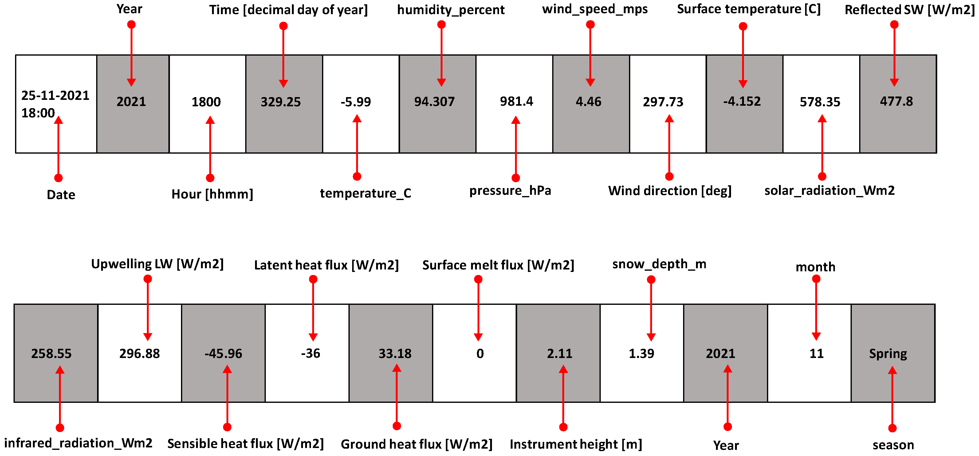
Figure 1. Overview of the Antarctic AWS dataset (2020–2024) showing sample entries with meteorological variables, timestamps, and derived features used for analysis.
Digital 05 00050 g001
Figure 2. Workflow of Antarctic climate data processing and analysis, including data acquisition, preprocessing, transformation, visualization, and modeling steps.
Digital 05 00050 g002
Figure 3. Model training results for temperature prediction using the constructed Python pipeline.
Digital 05 00050 g003
Figure 4. Average monthly temperature trends (°C) at the study station, showing characteristic austral seasonal variability.
Digital 05 00050 g004
Figure 5. Yearly average temperature (°C) at the study station for 2021–2024, indicating interannual fluctuations.
Digital 05 00050 g005
Figure 6. Temporal variation in snow depth (m) from 2022 to 2024, illustrating seasonal accumulation and compaction.
Digital 05 00050 g006
Figure 7. Time series of incoming solar radiation (W/m2) from 2022 to 2024, highlighting the pronounced annual cycle of insolation at the station.
Digital 05 00050 g007
Figure 8. Spearman correlation matrix of meteorological variables at the study station (2020–2024). The matrix shows both color intensity and numerical values of Spearman’s ρ , with variables labeled using standardized units. Values closer to ± 1 indicate stronger monotonic associations.
Digital 05 00050 g008
Figure 9. Lead–lag cross-correlation analysis between temperature and solar radiation anomalies, illustrating potential temporal offsets in their relationship.
Digital 05 00050 g009
Figure 10. Comparison of Linear Regression and Random Forest performance using R 2 , RMSE, and MAE metrics.
Digital 05 00050 g010
Figure 11. Random Forest feature importance ranking for near-surface temperature prediction, showing the contribution of radiative and thermodynamic variables.
Digital 05 00050 g011
Table 1. Summary of Recent Studies on Antarctic Sea Ice Prediction.
YearAuthorTitle (Short)Method(s)Key ResultsContributionLimitation
2023Koerich et al. [14]SIPN South Initial ResultsMulti-group seasonal forecast intercomparisonEnsemble median captures negative anomalies well; observations within forecast spreadDemonstrates collaborative ensemble skill for Antarctic predictionRoss Sea bias; ensemble spread remains large
2022Tewari et al. [15]Early Predictability EstimatesCCSM3 ensemble, idealized perturbation testsFound 3–9 month predictability windows; seasonal re-emergence of predictabilityProvided first model-based timescales for Antarctic predictabilityOnly model-based; lacks direct real-world verification
2024Maniraj et al. [16]Observational Skill AssessmentStatistical models, linear Markov, hindcastsUp to 1-year skill for regional ice concentration; strong seasonal differencesDemonstrates empirical forecast potential using reanalysisSparse observational data limits skill
2023M. Casado [17]Regional Mechanisms (Wind–Ice Link)Reanalysis link analysis, dynamical-statisticalZonal wind anomalies linked to late summer Ross Sea ice; 5-month lag foundIdentifies physical driver for regional predictabilityMechanism not robust across models
2023Nicola et al. [18]Thickness InfluenceCoupled dynamical hindcasts with initializationIncluding ice thickness boosts forecast skill; Weddell Sea shows longest horizonHighlights importance of thickness for skillful predictionScarcity of reliable thickness data
2023King et al. [19]S2S System EvaluationS2S forecasts, strict edge metricsExisting S2S systems rarely beat climatology beyond weeksUnderscores gap in current S2S systems for Antarctic iceLimited polar-specific system design
2022Strugnell et al. [20]Ocean Mixed Layer InfluenceMulti-GCM ensemble intercomparisonDeeper mixed layers lengthen predictability horizon; ocean vertical structure keyShows oceanic processes are crucial for sea ice memoryHigh model spread; regional differences large
2022Blazsek et al. [21]Arctic vs. Antarctic ContrastIdealized model intercomparisonAntarctic sea ice less sensitive to volume initialization than ArcticProvides important polar intercomparison baselineLimited region-specific detail
2023Massonnet et al. [22]New Regime DetectabilityHindcast covering record lows periodRecent higher variance extends skill horizon vs. pastSuggests current conditions may aid longer skill windowsShort satellite record constrains conclusions
2022Holland et al. [23]SIPN South Open Data ResourceShared community repositoryForecasts and verification data openly accessible for polar community useSupports further development and policy-relevant researchData gaps in some regions
Table 2. Descriptions of dataset variables.
Dataset VariableDescription
dateTemporal information for each observation.
HourPrecise timestamp indicating the hour and fractional part of the day.
YearCalendar year to facilitate comparison across years for climate trend analysis.
Time [decimal day of year]Time expressed as a decimal fraction of the day within the year (e.g., 32.5 = noon on day 32).
Temperature [°C]Air temperature in ° Celsius.
Humidity_PercentRelative humidity expressed as a percentage.
pressure_hPaAtmospheric pressure measured in hectopascals (hPa).
wind_speed_mpsWind speed measured in meters per second.
Wind direction [deg]Direction from which the wind blows, in degrees (0 = North, 90 = East, etc.).
Surface temperature [°C]Temperature measured at the surface in ° Celsius.
solar_radiation [W/m2]Incoming shortwave solar radiation in watts per square meter (W/m2).
Reflected SW [W/m2]Reflected shortwave radiation in watts per square meter (W/m2).
infrared_radiation_Wm2Incoming longwave (infrared) radiation from the atmosphere.
Upwelling LW [W/m2]Outgoing longwave radiation emitted from the surface.
Sensible heat flux [W/m2]Heat exchange between the surface and atmosphere due to temperature differences.
Latent heat flux [W/m2]Heat exchange caused by water phase changes, such as evaporation or condensation.
Ground heat flux [W/m2]Heat transfer between the surface and subsurface ground.
Surface melt flux [W/m2]Energy flux related to melting occurring at the surface.
Instrument height [m]Height of measurement instruments above the surface.
snow_depth [m]Depth of snow on the surface measured in meters.
YearDuplicate of the calendar year for reference.
MonthCalendar month of the observation.
SeasonMeteorological season corresponding to the month (e.g., Winter, Spring, Summer, Fall).
Disclaimer/Publisher’s Note: The statements, opinions and data contained in all publications are solely those of the individual author(s) and contributor(s) and not of MDPI and/or the editor(s). MDPI and/or the editor(s) disclaim responsibility for any injury to people or property resulting from any ideas, methods, instructions or products referred to in the content.