Using Machine Learning Techniques for Asserting Cellular Damage Induced by High-LET Particle Radiation

Abstract

This is a study concerning the use of Machine Learning (ML) techniques to ascertain the impacts of particle ionizing radiation (IR) on cell survival and DNA damage. Current empirical models do not always take into account intrinsic complexities and stochastic effects of the interactions of IR and cell populations. Furthermore, these models often lack in biophysical interpretations of the irradiation outcomes. The linear quadratic (LQ) model is a common way to associate the biological response of a cell population with the radiation dose. The parameters of the LQ model are used to extrapolate the relation between the dosage and the survival fraction of a cell population. The goal was to create a ML-based model that predicts the $\alpha$ and $\beta$ parameters of the well known and established LQ model, along with the key metrics of DNA damage induction. The main target of this effort was, on the one hand, the development of a computational framework that will be able to assess key radiobiophysical quantities, and on the other hand, to provide meaningful interpretations of the outputs. Based on our results, as some metrics of the adaptability and training efficiency, our ML models exhibited 0.18 median error (relative root mean squared error (RRMSE)) in the prediction of the $\alpha$ parameter and errors of less than 0.01 for various DNA damage quantities; the prediction for $\beta$ exhibited a rather large error of 0.75. Our study is based on experimental data from a publicly available dataset of irradiation studies. All types of complex DNA damage (all clusters), and the number of double-stranded breaks (DSBs), which are widely accepted to be closely related to cell survival and the detrimental biological effects of IR, were calculated using the fast Monte Carlo Damage Simulation software (MCDS). We critically discussed the varying importance of physical parameters such as charge and linear energy transfer (LET); we also discussed the uncertainties of our predictions and future directions, and the dynamics of our approach.

1. Introduction

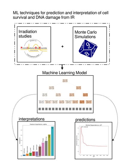
When a population of living cells is exposed to ionizing radiation (IR), an array of complex responses takes place. Our main aim was to predict the irradiation’s effect on the survival of cells and its impact on the cell’s DNA. In order to achieve this, we employed various Machine Learning (ML) techniques and fast Monte Carlo simulations [1] to calculate the DNA damage. 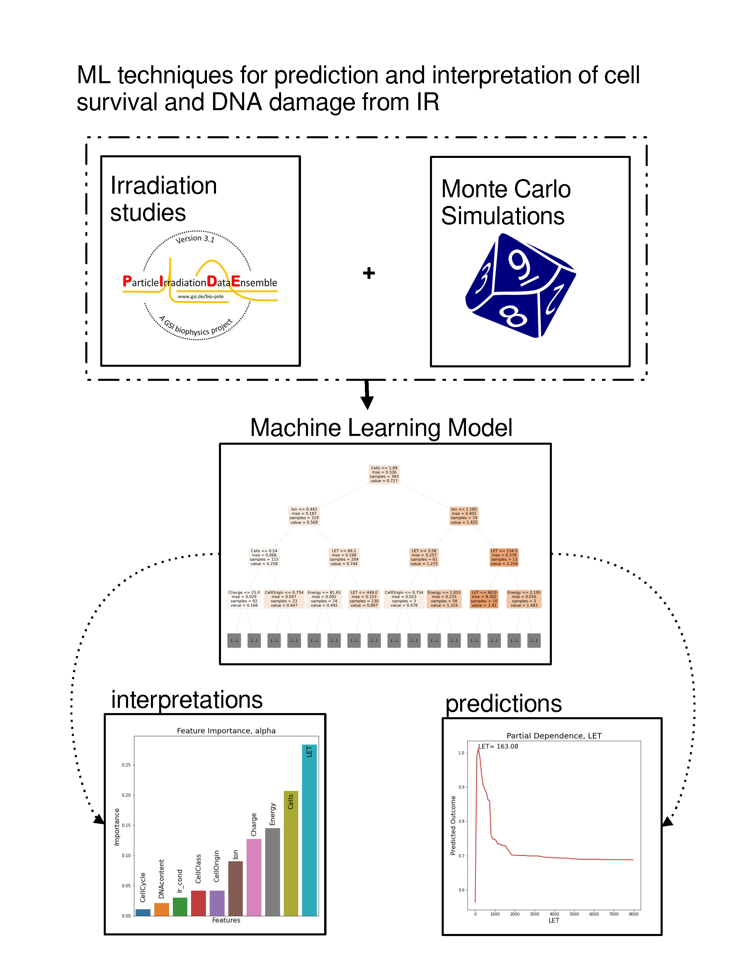The study was based on an extended dataset of cell irradiation studies: PIDE [2]. This introduction aims to illustrate the biophysical importance of the dataset’s features and their impacts on the biological outcome of the computational model itself. Additionally, the basic rationale of the ML approach is outlined. A common way of modeling and quantifying the relation between radiation dosage and fraction of surviving cells is the established linear quadratic (LQ) model.

1.1. LQ Model

The LQ model [3] is among several empirical and less mechanistic mathematical formalisms that have been proposed to describe the relation between cell survival and radiation dose absorption by cells or tissues. It is also among the most prevalent models in this field, and its basic assumption is that there are two parameters that contribute to cell killing: the first, $\alpha$, is mainly the linear component and relates to the dosage D, while the second $\beta$, a quadratic component relates to the square of the dosage $D^2$ [4]. This relation is expressed in the equation: $S\left(D\right)=e^{-(\alpha D+\beta D^2)}$ where S represents the fraction of cells that survived dose D. In Figure 1 below, a typical response curve of a cell population to ionizing radiation based on the LQ model is presented as an example.

The $\alpha$ and $\beta$ parameters represent the linear and quadratic contributions to cell death, respectively. The LQ model’s widespread usage lies in the fact that it has only two parameters and it is not computationally demanding. These parameters also have some associated biophysical importance and biophysical interpretations [4]. Single hits of radiation (one particle) may cause cell death by inducing breaks in two adjacent chromosomes ($\alpha$D component). When two or more particles induce two chromosomal breaks, injuries become cumulative. Irradiation’s mechanism behind cell death is believed to be strongly related to DNA damage, and double-stranded breaks (DSBs) especially [5]. The probability of this multiple-hit event is proportional to the square of the dose, which is represented by the $\beta$ parameter. A significant part of this study is the determination of the dose–response of a cell population, by predicting the $\alpha$ and $\beta$ parameters of the LQ model.

1.2. Radiation Properties

Linear energy transfer (LET) is a quantity that signifies the average amount of energy that ionizing radiation conveys to a material, per unit of distance. It describes the transfer of radiation’s energy to matter; it depends on the nature of the irradiated matter, and the type of radiation and its characteristics, such as particle kinetic energy and charge, but it is strictly positive. Energy transfer causes damage to the structure of the material, as near the radiation track the ionizing particle contacts the material. In biological systems, such microscopic failures increase the chance of a large scale failure, such as a double-stranded DNA break or cell apoptosis. LET’s importance stems from the fact that DNA damage is not proportional to the absorbed dose and it is typically measured in KeV/$\mathsf{\mu }$m or MeV/mm. Another aspect of the impact of IR on cells is the number of DSBs induced by that radiation. In this study, we predict DSBs and all types of complex DNA damage (all clusters). Both all clusters and DSBs are measured in number of lesions per Gray per ${10}^9$ bp i.e., $Gra{y}^{-1}\ast Gb{p}^{-1}$. DNA damage was calculated through fast Monte Carlo simulations. There are several different ways to quantify the complexity of DNA damage, from defining a single DSB as a region in which two DNA lesions exist within a span of less than 10 base pairs (bp), to incorporating other types of critical damage to the DNA molecule in a region sufficiently close to a DSB, which amounts to what we describe as all clusters. The all clusters metric is described in detail in the Methods section.

1.3. Biophysical Background

This study includes two categories of features. On one hand, there are physical features related to the radiation itself, such as LET and ion species. On the other hand, there are biophysical features related to the cell, such as cell cycle phase, cell line and cell type (i.e., normal or tumor). A high LET value denotes quick attenuation of the radiation inside the material, lower radiation penetration and increased complexity of damage [6]. From a biological standpoint, such microscopic failures increase the chances of large-scale failures, such as double-stranded DNA breaks and cell apoptosis. Radiation affects cells in multiple ways, including cellular damage, apoptosis, mutations and chromosome aberrations, i.e., genomic instability. Cells exhibit varying responses to low doses of radiation which cannot be extrapolated accurately from high-dose responses to low dose radiation, a state that can lead to low-dose hyper-radiosensitivity (HRS) and increased radio resistance (IRR). The phase of the cell cycle and whether the cell is tumorous or not are considered to play major roles in radiosensitivity.

1.4. Machine Learning Approach

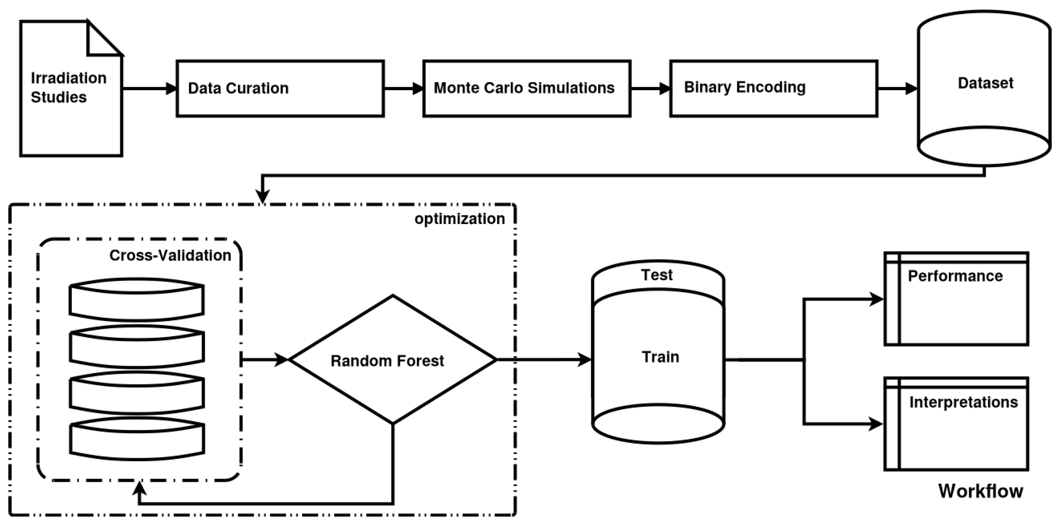
In the case of cell irradiation there can be no specific hypothesis for the variable distribution, as features exhibit complex multicollinearities and there is also a strong element of randomness (intrinsic noise) in the studied data. Based on the above, we are compelled to implicate ML methods. ML, in contrast to classical statistics, does not impose a preconceived relation between dependent and independent variables. ML aims to “learn” the dataset itself. In this study, we will adhere to what in statistics are called independent and dependent variables as features and targets respectively, in compliance with ML lingo. The random forest [7] (RF) algorithm that was chosen is typical for ML models, but it produces a “black box” model. This means that it does not offer any biophysical explanations for its predictions. In order to overcome this opaqueness of ML models and interpret the relations between the features and the outcome, various interpretation methods are employed, such as surrogate models and partial dependencies. In fact, predictive performance is used as a quality indicator for the interpretations.

2. Results

Model assessment is organized into two sections. Firstly, several metrics and graphs that quantify the predictive performance of our model are presented. Evaluation of the implementation of the model can be done along various lines. Here, some basic evaluation aspects are presented, such as confidence intervals and the distribution of true vs. predicted values. The next section of results accommodates their interpretation, such as feature importance, interactions and individual prediction interpretation graphs. The terms a_paper, b_paper, a_fit and b_fit below refer to the way that $\alpha$ and $\beta$ parameters are represented in the dataset. The difference between paper and fit targets is that the former refer to parameters as they were measured and calculated by the authors in the original studies of the dataset, while the latter refer to their calculations through fitting, based on cell survival data from the creators of the PIDE database [2]. In this section, two kinds of result plots are presented:

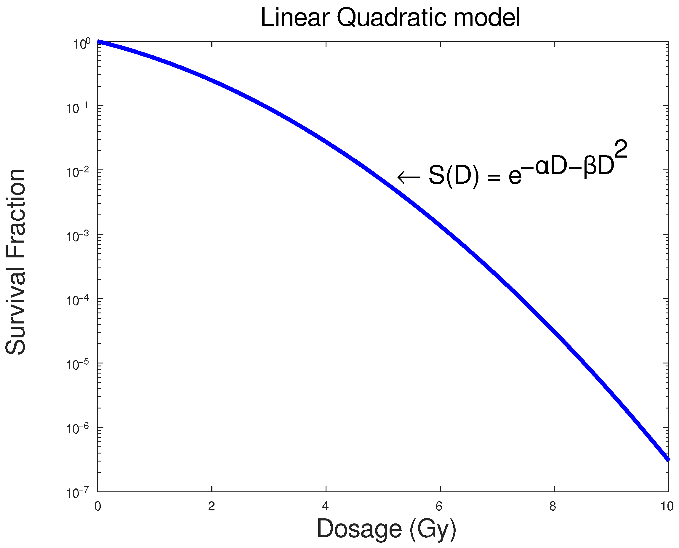
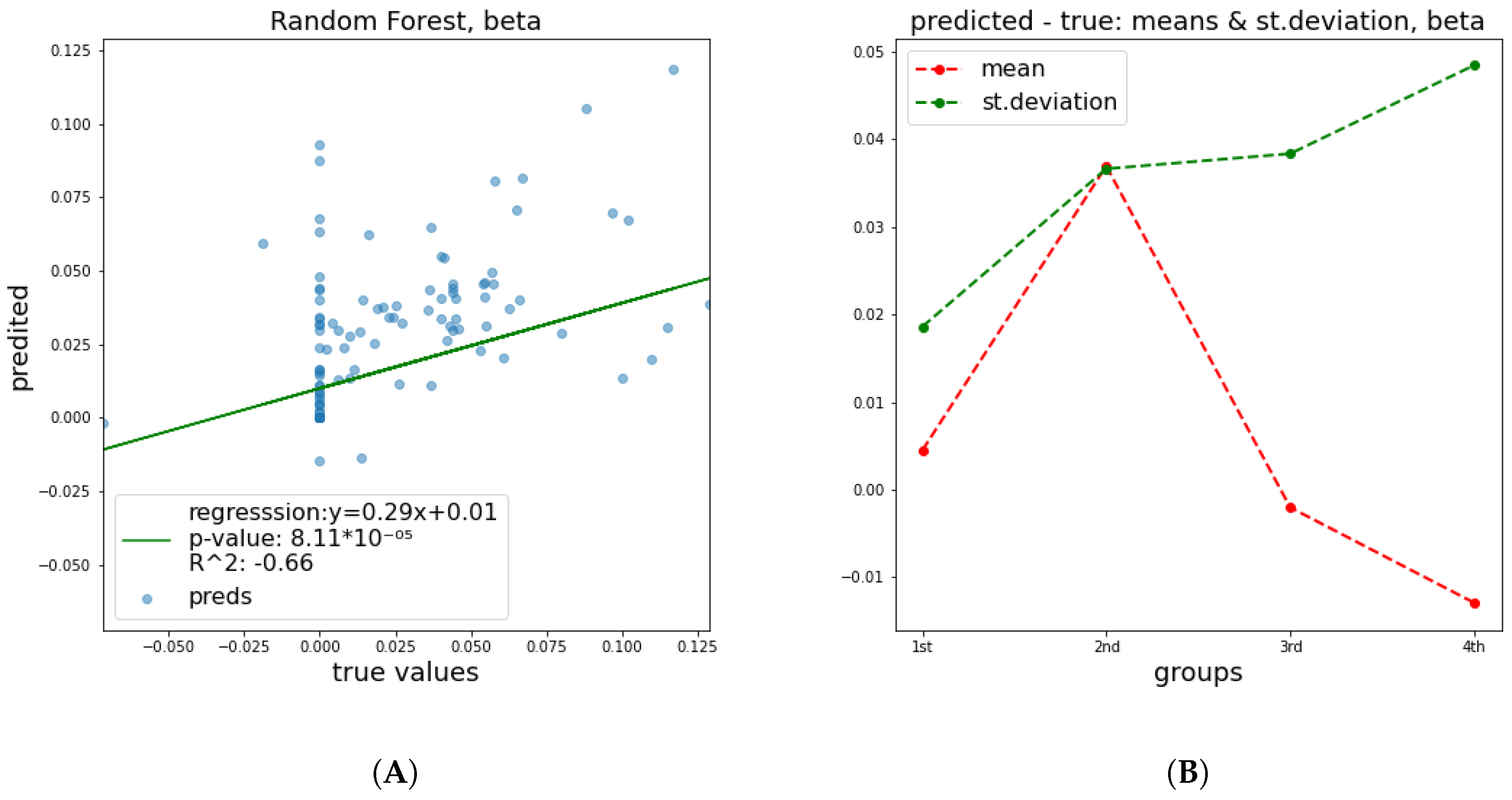
• True vs. predicted graphs show the evolutions of key statistics in every ML model. These graphs consist of pairs of actual and predicted values from the test set, on which the model was not trained (holdout set). The closer these points are to the $y=x$ line, the better the predictive performance of the estimator. Additionally, a linear regression line was plotted based on the points in order to quantify the distance from the identity line, with the corresponding equation being given on the plot. p-values represent the probability that, given the sampled data, the slope of the regression line is zero—i.e., that the two variables are unrelated.
• Mean and standard deviation graphs depict the ways in which the means and the standard deviations (STD) of error change. The pairs of true and predicted values were sorted with respect to the true value and they were separated into four groups containing equal numbers of pairs. For each group, the means and the STD of distance between the two parts of the pair (i.e., error) were calculated. This graph aims to examine whether the error of the ML model follows a specific trend. The x-axis corresponds to the four groups of errors, while the y-axis has the same units as the target studied.

For brevity, only the figures related to a_paper and b_paper are included, because based on the results of

Table 1. Predictive performance for $\alpha$ and $\beta$ parameters.

Targets	Lower Percentile	Median	Upper Percentile
a_paper	0.13	0.18	0.31
b_paper	0.41	0.75	1.0
a_fit	0.21	0.33	0.5
b_fit	0.63	0.85	1.0

, the performance falls significantly in the fitted cases.

2.1. Predictive Performance

2.1.1. $\alpha$ and $\beta$ Parameters

To describe the performance of estimator, the relative root mean squared error (RRMSE) metric is provided along with bootstrapped [8] 95% confidence intervals. The results in all tables that contain confidence intervals, for instance, see Table 1 below, are dimensionless and can be compared in each case.

What should become apparent from the above table is the better performance of our ML-based model regarding the $\alpha$ parameter, especially regarding the $\alpha$ parameter derived from experimental values of previous studies compared to those derived from the fitting process, as performed by the authors of PIDE database. The same trend was observed for the $\beta$ parameter, with the notable difference that in both paper and fit cases, predictions were altogether relatively bad, which is very informative about the nature of $\beta$. This is indicative of the fitting process, in which both of parameters increase the error. It also shows that the mean magnitude of the $\beta$ parameter is comparable to the measurement error and the fitting process error. The same picture arises when visualization of the estimator’s behavior is attempted. Especially for $\beta$ parameter, both the error and the graphs show a relation between the features and a value of $\beta$ that is close to random noise. The mean and standard deviation plots in all cases illustrate the same trend, namely, that the STD of distance between true and predicted values becomes larger, meaning that as the value that we are trying to predict increases, the error increases too. Figure 2 and Figure 3 depict the predictive performance of $\alpha$ and $\beta$ parameters. Additional results regarding the $\beta$ parameter that are related to further investigation of the model, such as partial dependence and various interpretation plots, are kept in the supplementary section (Figures S1 and S2).

2.1.2. DNA Damage

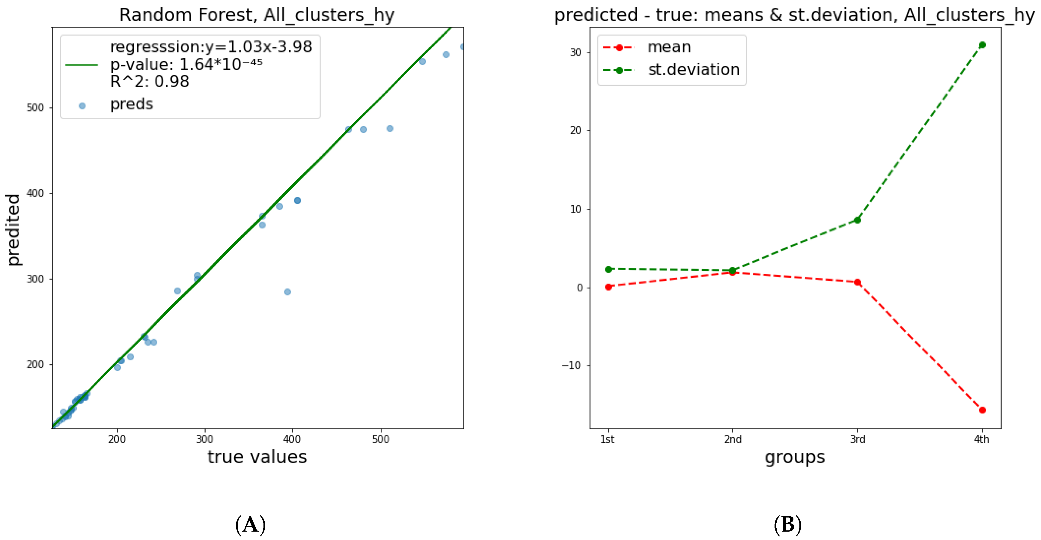
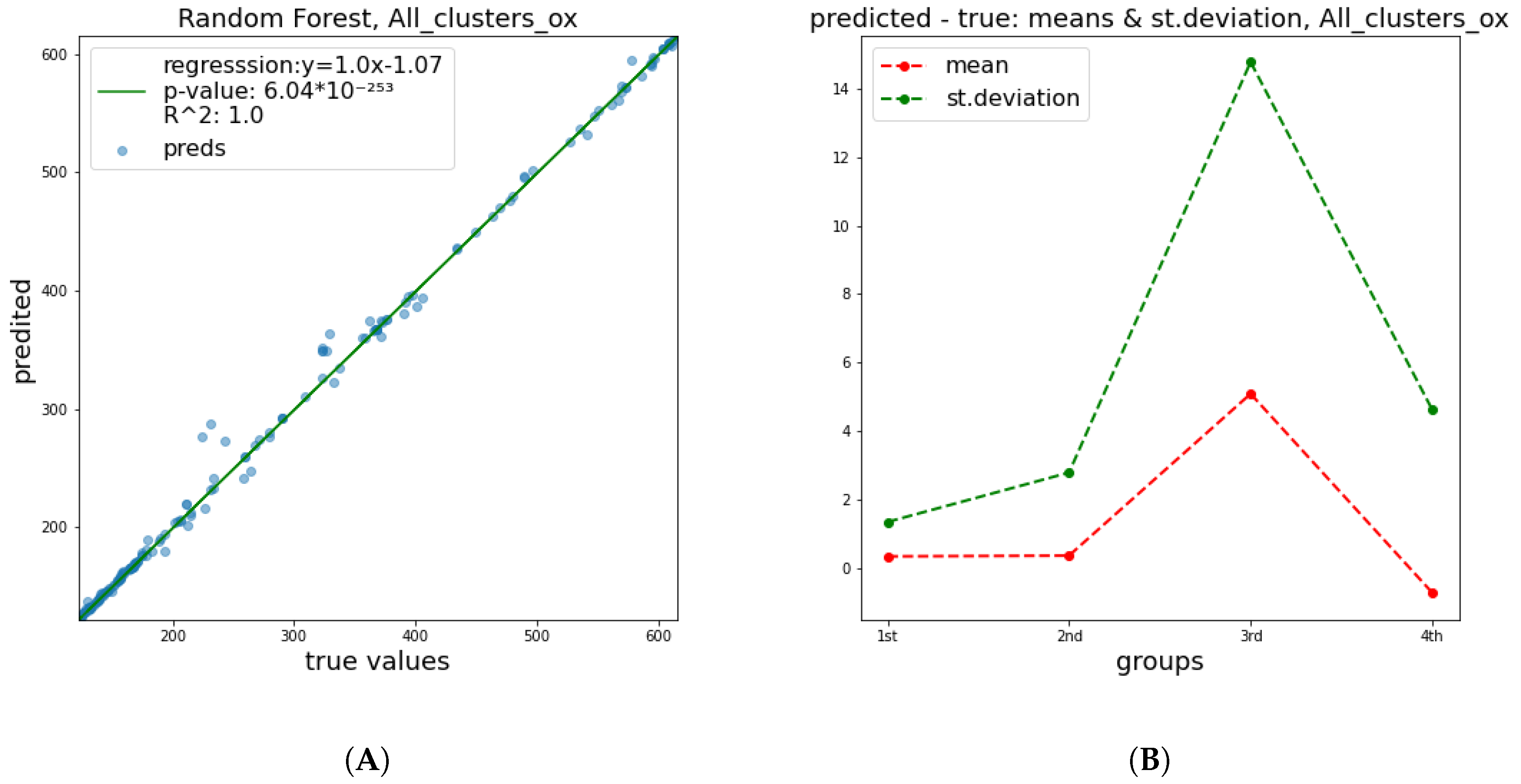
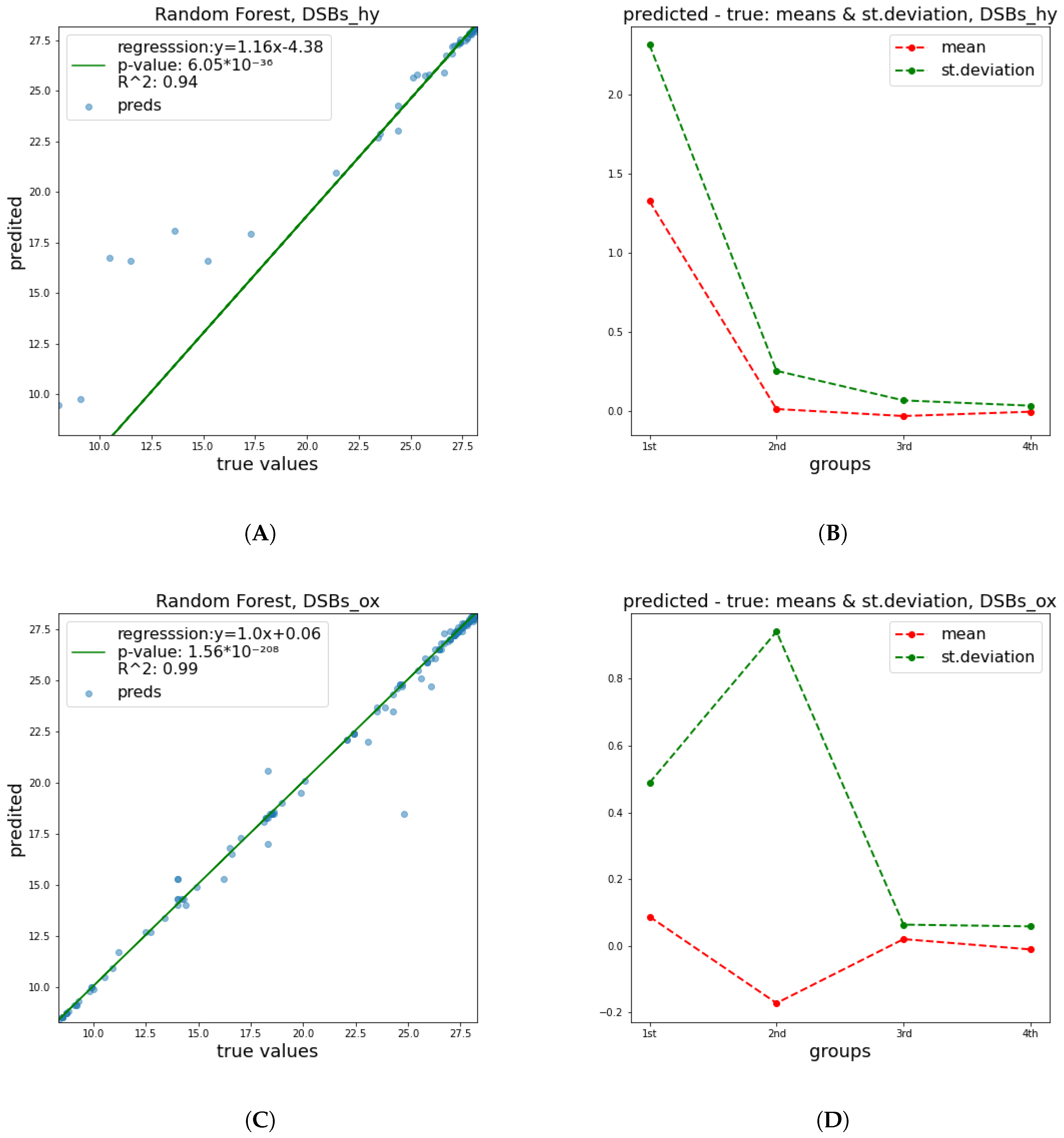
Similarly, the same metrics and visuals are provided for the predicting of DSB clustering damage of the DNA molecules (

Table 2. Predictive performance for DNA damage types.

Targets	Lower Percentile	Median	Upper Percentile
All Clusters (hypoxic)	0.076	0.089	0.100
All Clusters (oxic)	0.0005	0.0013	0.0029
DSBs (hypoxic)	0.059	0.066	0.073
DSBs (oxic)	0.031	0.034	0.036

).

These results show a significant improvement of the quality of predictions in relation to $\alpha$ and $\beta$ parameters. This happened mainly due to the fact that the breaking of a DNA strand is more attributable to a small number of radiation features and has a less complex nature, in contrast to cell apoptosis, which is affected by a numerous factors, including biological DNA repair mechanisms and genes’ functions or possible deficiencies. Therefore, it is easier to predict the damage of DNA molecule. In Figure 4, Figure 5 and Figure 6 below, corresponding plots for the DNA damage features that underline the effect of the improvement shown in the previous table are provided. Additionally, it is apparent that the error of prediction increases for greater values of all clusters.

2.2. Interpretation

2.2.1. Feature Importance

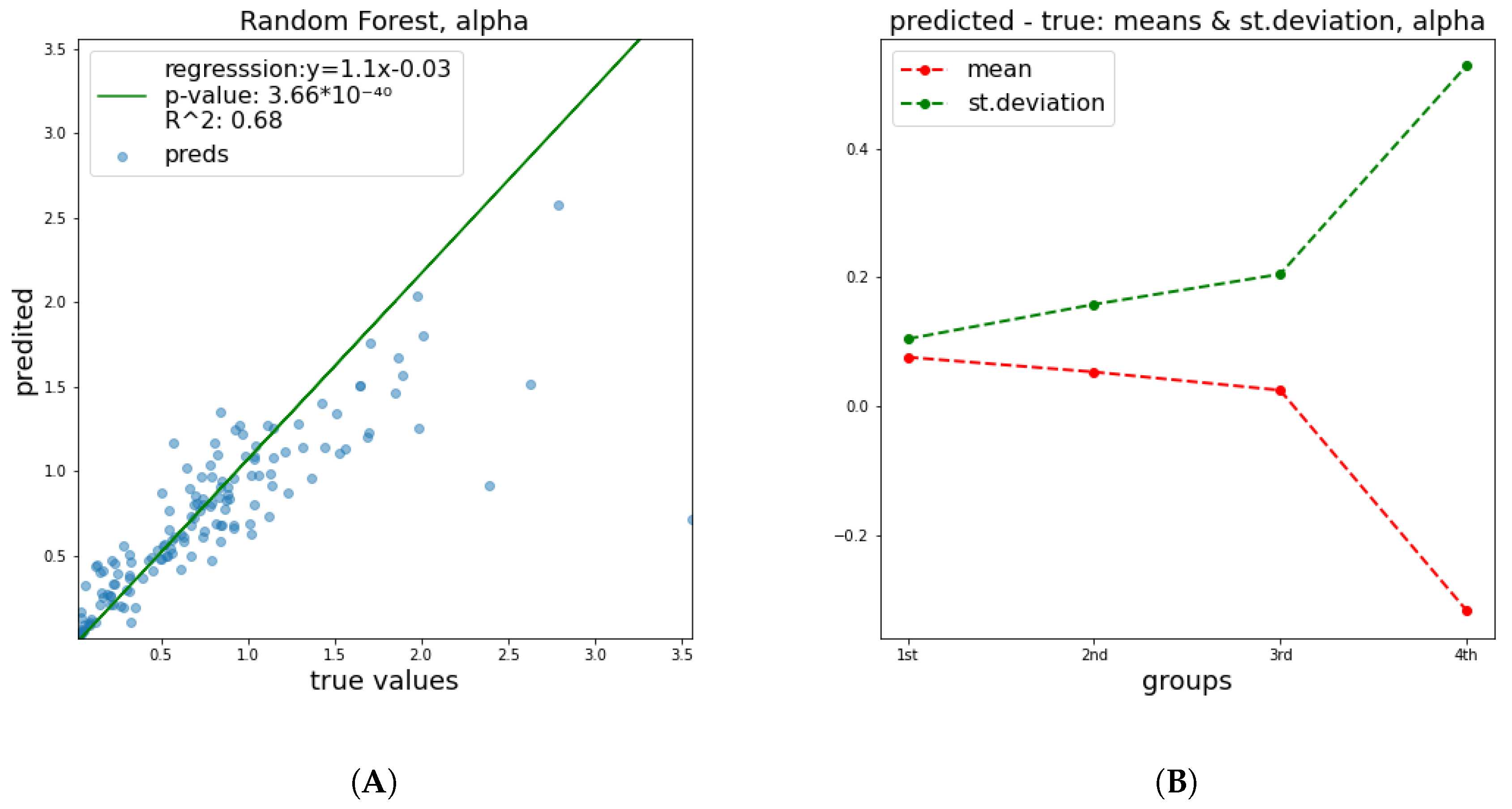
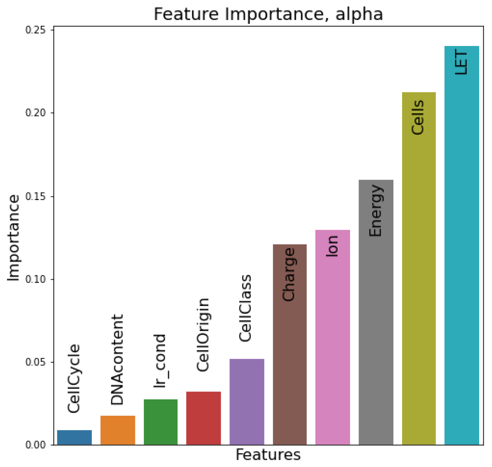
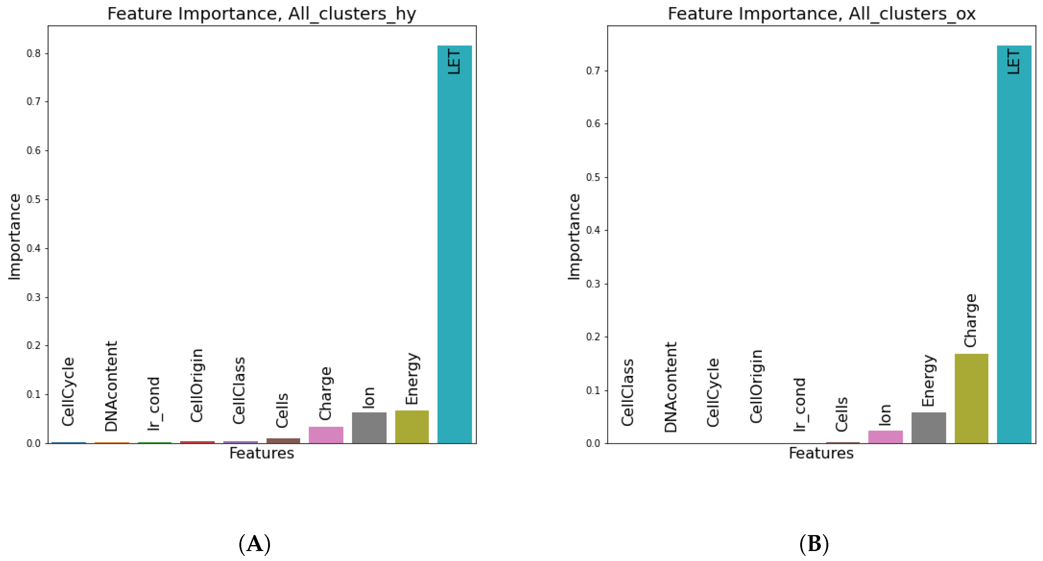
In this section, the relative importance of features in the dataset is presented. In the first case (Figure 7) of the $\alpha$ parameter, LET and cell line features seem to be the most determinant factors to the prediction of the estimator, followed by energy and ion species features. In Figure 8, LET seems to be by far the most instrumental feature (as expected) in predicting the number of all clusters in both oxic and hypoxic cases.

2.2.2. Partial Dependence

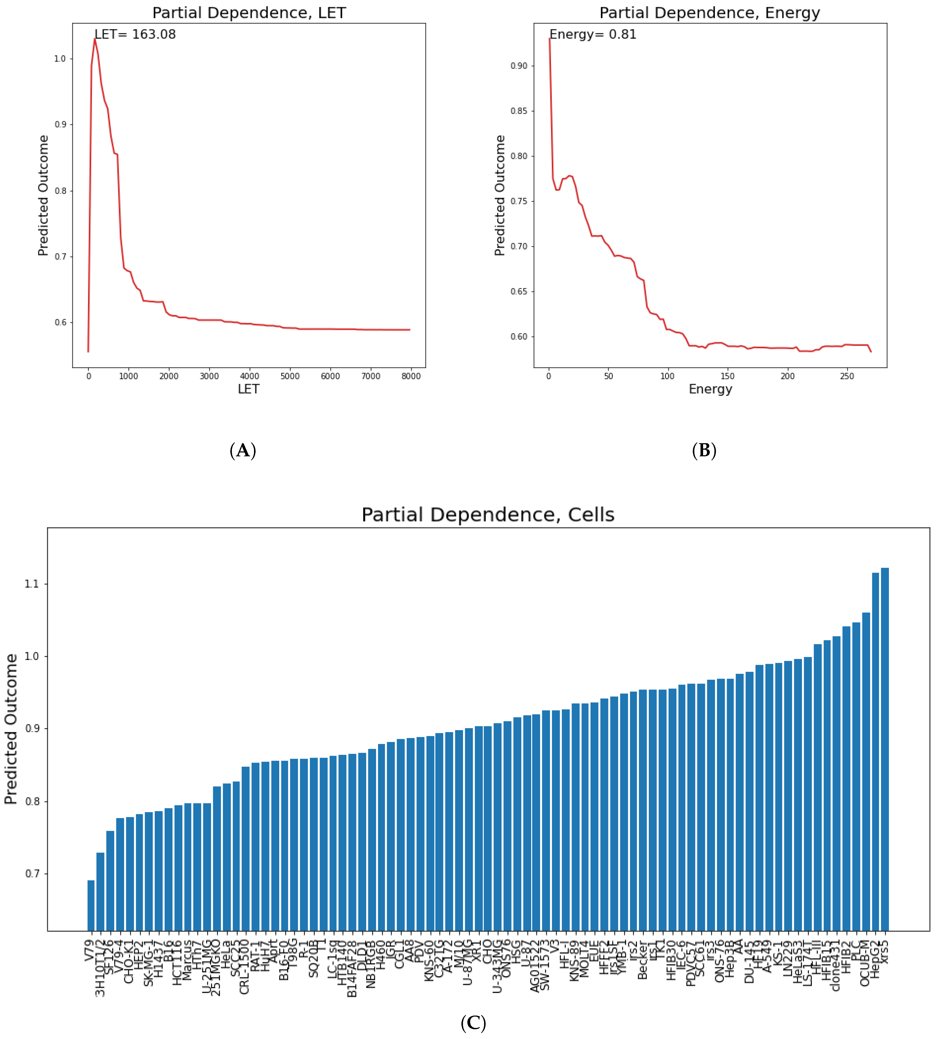
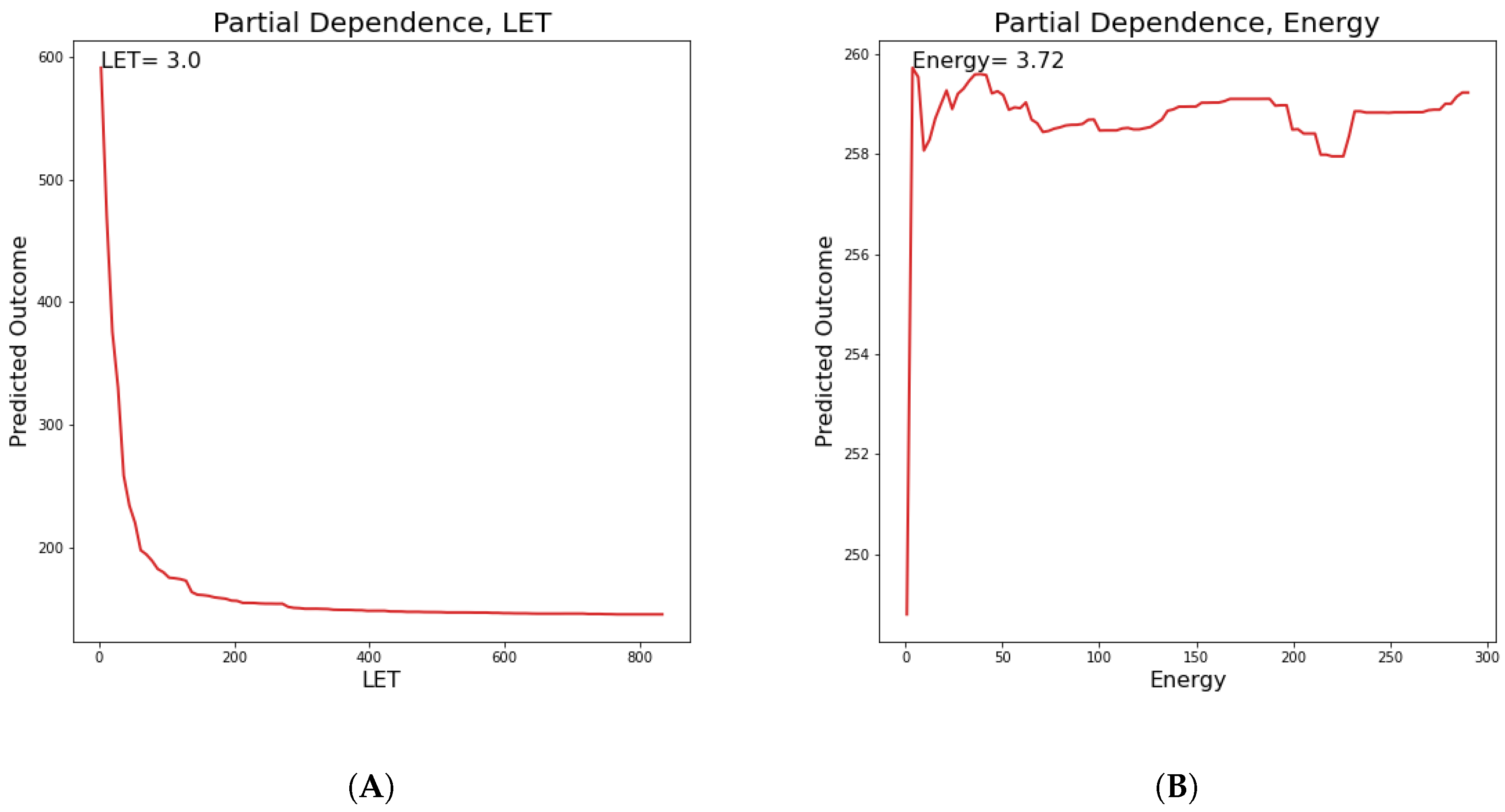
In this section, partial dependence plots are presented concerning all the predicted targets for the three most important features. A partial dependence plot depicts the impact of one or multiple features on the predicted target. It can also reveal whether the relation is linear or more complex. In linear regression, the plot should be a straight line. In this way, partial dependence plots can give valuable insights to biophysical modeling. Additionally, for continuous features, the value of the feature where the predicted outcome is maximum is provided. We will discuss results regarding the $\alpha$ parameter, so as to illustrate how plots like these should be interpreted. LET, cell lines and Energy partial dependence plots are shown below (Figure 9). Concerning LET, the predicted outcome is reaching a maximum value of 163.1 KeV/$\mathsf{\mu }$m and falls rapidly into a steady state. For the cell line, it appears that there are groups of cell lines which have the same or very similar predicted outcome, which reaches a maximum for cell lines xrs5, KS-1 and IGR.

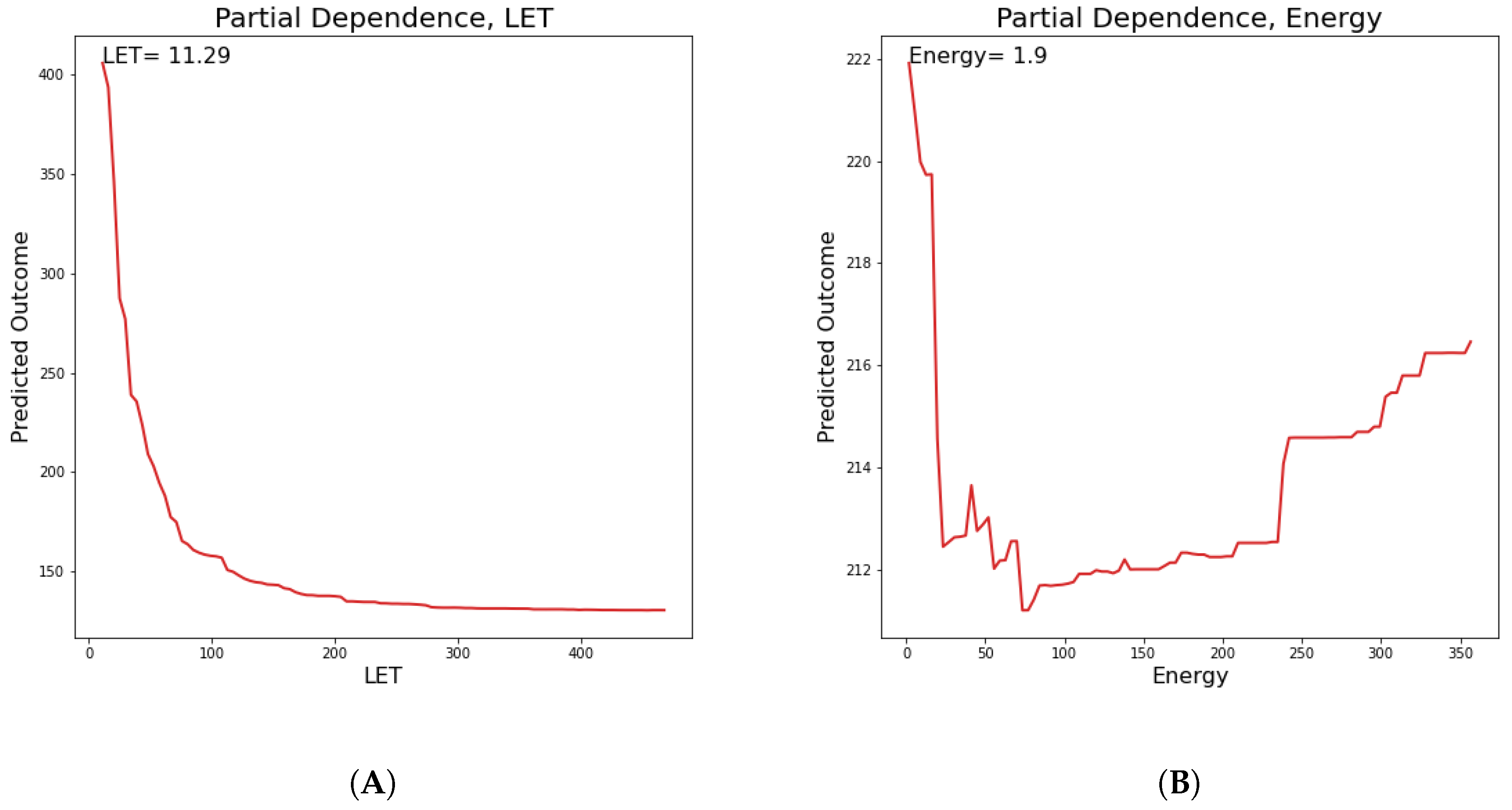
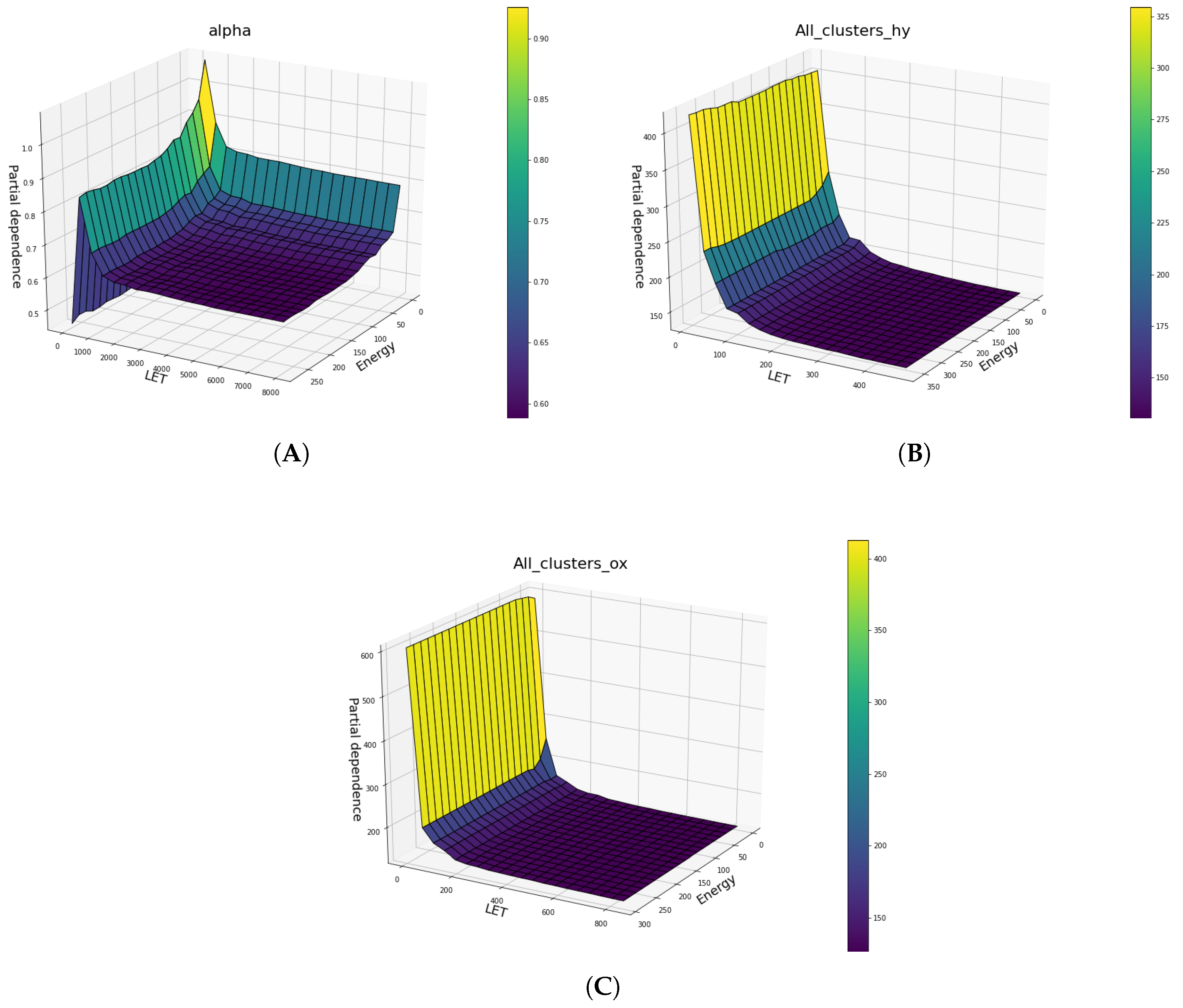
Below in Figure 10 and Figure 11, the partial dependences of all clusters DNA damage in hypoxic and oxic cells on the LET and specific energy features are presented.

Below (Figure 12), several two-way Partial Dependence plots between LET and energy features, which are both continuous features and its comparison is meaningful, are shown, illustrating how the two features influence in tandem the predicted outcome. This produces a three dimensional plot where the two base axes correspond to the two features, and the vertical axis corresponds to the predicted outcome.

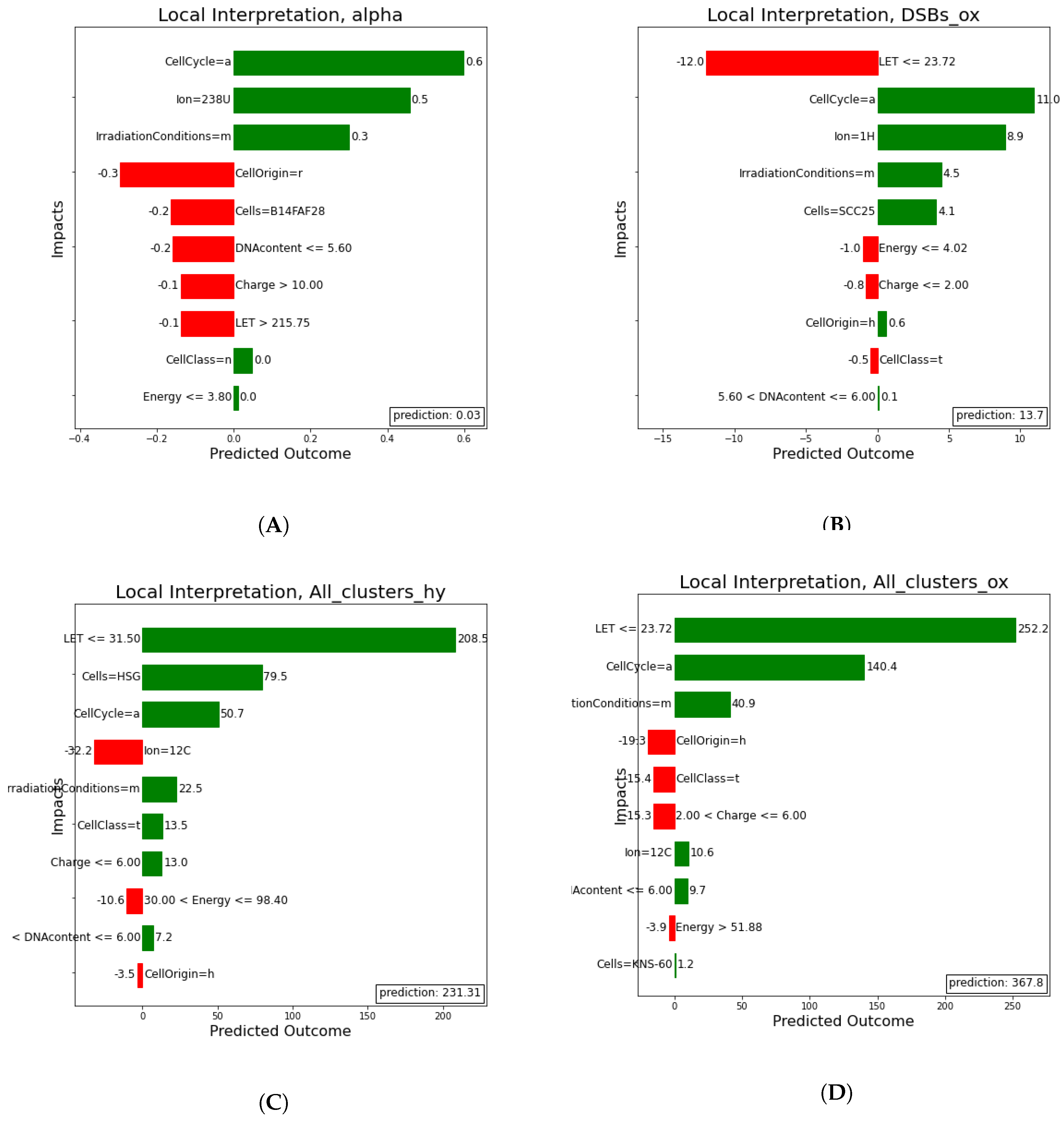
2.2.3. Local Interpretation

Here, (Figure 13) a local rule-based interpretation of individual predictions is shown. The plots depict an explanation of the predictions of four irradiation experiments, based on specific values of the features in a descending order of significance. The direction of the bar, signifies whether the feature has a negative or positive effect on the predicted outcome (left being negative and right positive). In

Table 3. Prediction of individual sample.

Targets	Prediction	True Value
$\alpha$ parameter	1.92	2.2
DSBs oxic	13.7	13.7
All Clusters (hypoxic cells)	231.8	231.0
All Clusters (oxic cells)	367.1	367.8

below, the exact values predicted in comparison to the true values on which the local prediction interpretations were made, are shown.

2.3. Significance Analysis

To establish whether the ML model has statistically significant better performance than a classic statistical method, several statistical models were also fitted and compared to the ML model. Here (

Table 4. Statistical significance. H0: the means of the error distribution that ML model produces are significantly different from that of a classic statistical model.

Targets	p-Value	Result
$\alpha$ parameter	1.8 × 10−5	reject H0
$\beta$ parameter	9.4 × 10−1	fail to reject H0
All Clusters (hypoxic cells)	1.5 × 10−7	reject H0
All Clusters (oxic cells)	4.2 × 10−11	reject H0
DSBs (hypoxic cells)	5.4 × 10−6	reject H0
DSBs (oxic cells)	1.0 × 10−9	reject H0

), the results from this comparison with the statistical model that fared better, which is the generalized linear model [9] with Poisson link function, are presented.

Several link functions were tried, among which the Poisson fared better. Linear regression assumes that the dependent variable is normally distributed. GLMs can have dependent variables distributed in other ways, not necessarily by following Normal distribution and the relationship between independent and dependent variables can have a non-linear form. The link function links the mean of the dependent variable $Y_i$ which is $E\left(Y_i\right)={\mu }_i$ to the linear term $x_i^T$ through a link function $g\left({\mu }_i\right)=x_i^T$. This approach seems to be the most appropriate for our task, given the nature of the responses of Cells to radiation, which is not linear.

The ML model consistently produced lower mean errors. The question is, whether there is significant difference in the error distribution, and by what margin. Hypothesis H0 is that the means of error distributions do not differ significantly. For all targets, the ML model displayed significantly better performance compared to any classic statistical model, as indicated by the respective p-values by orders of magnitude, with the exception of the ML model trained for $\beta$ parameter, where the rejection of H0 hypothesis indicates that our model does not manage to improve the prediction in relation to the statistical model, with a cutoff value of 0.05. This last point is another sign of the inherent noise and large uncertainty in $\beta$ parameter and indicates that both ML and statistical models are similarly bad at predicting the $\beta$ parameter

3. Materials and Methods

3.1. The Data

The dataset originates from a compilation of cell survival studies, spanning decades, gathered and curated by the Particle Irradiation Data Ensemble (PIDE) dataset provided by the GSII [2]. Dataset pide_3.2 consists of 1150 samples of radiobiological studies, including key cellular and radiation features. Among results, there are the $\alpha$ and $\beta$ parameters of LQ model. The dataset is complemented with DNA damage features, calculated for each sample by the Monte Carlo method cited below. The $\alpha$ and $\beta$ values are dimensionless, while all clusters and DSB values are measured in $\left(clusters\right)/Gray\ast Gbp$. Terms hypoxic and oxic refer to the concentration of oxygen in the simulation, where hypoxic corresponds to 3% oxygen conditions and oxic to 20% oxygen conditions. Three randomly chosen experiments are given below (

Table 5. Data Sample (features).

Features
Cell	Type	Origin	Phase	Genl	Ion	Charge	Irmods	LET	E
HF19	n	h	a	6.0	4He	2.0	m	20.0	8.80
R-1	t	r	a	5.6	12C	6.0	s	11.0	389.00
V79	n	r	a	5.6	1H	1.0	m	31.0	0.76

,

Table 6. Data Sample (targets).

Targets
$\mathbf{\alpha }$	$\mathbf{\beta }$	All Clusters Hypoxic$({\mathit{Gray}}^{-\mathbf{1}}\ast {\mathit{Gbp}}^{-\mathbf{1}})$	All Clusters Oxic$({\mathit{Gray}}^{-\mathbf{1}}\ast {\mathit{Gbp}}^{-\mathbf{1}})$
1.090	0.000	354.5	355.9
0.402	0.054	407.5	412.6
1.030	0.000	394.0	398.0

and

Table 7. Data explanation.

Var_Name	Description	Categorical\Numeric
Cells	Name of cell line	categorical
Type	Tumor cells (t) or normal cells (n)	categorical
Origin	human (h) or rodent cells (r)	categorical
Phase	Cell cycle phase (phases are given explicitly, or a for asynchronous)	categorical
Genl	Genomic length of diploid cells (in 10 bp, 5.6 for rodent and 6 for human cells)	numeric
Ion	Ion species	categorical
Charge	charge of ions	numeric
Irrmods	Irradiation modalities: monoenergetic (m) or spread out Bragg peak (s)	categorical
LET	Linear energy transfer in water (in keV/$\mathsf{\mu }$m, for irradiation in spread out Bragg peak dose mean or track averaged LET)	numeric
E	Specific energy of ions (in MeV/u), evaluated at the target	numeric

). The majority of samples were found to be related to oxic cells.

Each study reports its statistical errors, which indicates a lower limit to the uncertainty of the data. There is not a uniquely established way of reporting error in survival studies, which is why a broader uncertainty analysis is needed, for both statistical and systemic errors. The overall uncertainty could be determined by compiling larger datasets of experimental data from different laboratories, obtained under similar conditions. From such a dataset, the scatter of data would lead to an empirical measure of the uncertainty. This informs us that we deal with a task of learning a noisy dataset, which would be a good use case for a ML model.

3.2. Monte Carlo Damage Simulations (MCDS)

Based on the original dataset, a series of Monte Carlo simulations were performed in order to determine the amount of all clustering DNA damage. The MCDS fast MC software [1] was used, which provides a fast quasi-phenomenological method to interpolate damage yields from computationally taxing, but more detailed, track-structured simulations. To begin with, we used MCDS version 3.10a in order to make simulations using data from PIDE. For each simulation, we had to insert the input file certain parameters, such as the oxygen pressure of target cells (20% for oxic, 3% for hypoxic), the ions and its kinetic energy (in MeV), for each row. If the experiment included both oxic and hypoxic cells, we ran the simulation twice and saved both results. The DNA content of cell nucleus (in Gbp) and its diameter (in um) were constant, 1 and 5 for all the simulations. Nocs and seed, the “simulation control” parameters were constant too, 10,000 and 987,654,321. Consequently, we ran the program and focused on the number of clusters per cell from the output file, which means that our results were per Gbp and per Gray. The features of interest each time were the total number of all clusters, which can be divided as:

• DSB+ (DSB accompanied by one (or more) additional SB within 10 bp separation);
• DSB++ (more than one DSB whether within the 10bp separation or further apart);
• SSBc (fraction of complex damage (SSB+ and 2SSB) among SSBs);
• SSBcb (fraction of complex damage (SSB+ and 2SSB) among SSBs; base damage included);
• DSBc (fraction of complex damage (DSB+ and DSB++) among DSBs);
• DSBcb (fraction of complex damage (DSB+ and DSB++) among DSBs; base damage included).

3.3. Model Building Process

The process that we followed in order to build the estimator (Figure 14) is based on a classic approach in ML context, which involved:

• Find oxygen concentration from literature for each study in PIDE dataset.
• Perform Monte Carlo simulations to assess DNA Damage and complement dataset with corresponding metrics.
• Map categorical features to numerical values (categorical encoding) and remove null values.
• To optimize the model, i.e., to find the optimal hyper-parameters, we perform 5-fold cross-validation using a grid of possible hyper-parameters.
• Hyperopt algorithm is used to find the best parameters.
• Split the dataset to train and test subsets at 80/20 ratio.
• Calculate performance metrics of the optimized model and provide interpretations.
• Fit model to train set and compare results to test set, so as to assess performance and provide interpretation.

3.4. The Algorithm

To tackle the problem of predicting multiple continuous values from a single dataset, three methods were employed: Regression Chains, Stacking and Clustering [10]. The first two are similar and train a model to predict a single target at a time, while combining the predictions at a later stage. Clustering regression approach attempts to predict all the variables at once. These methods did not offer any significant advantage, while adding to training time. For this reason a single target regression model was used. The core of our method is the Random forest algorithm (RF) [7], as implemented in Scikit-Learn [11]. RF is a powerful and popular supervised learning algorithm. The “forest” that it builds, is an ensemble of decision trees usually trained with the “bagging” method. The general idea of the bagging method is that a combination of learning models improves the overall performance. It allows quick identification of significant information from extremely large datasets. The most important advantage of RF is that it relies on a collection of various decision trees to arrive at any solution. RF also adds additional randomness to the model, while growing the trees. Instead of searching for the most important feature when splitting a node, it searches for the best feature among a random subset of features. This results in a wide diversity that generally leads to a better model. While one of the biggest problems in ML is over-fitting, RF algorithm is particularly insensitive to it. Provided that there are enough trees in the forest, the model will not be subject to over-fit. RF is also robust to outliers and works well with non-linear data too.

3.5. Model Optimization

ML algorithms typically involve numerous user-defined parameters (hyper-parameters) that must be tuned in order to optimize their predictive performance. All possible combinations of hyper-parameters of a model form a parameter space or parameter grid. We chose not to brute-force our way through all possible permutations of the parameter space, assessing their performance. Instead, a bayesian method [12] that keeps track of previous evaluations was employed. The method uses past results to build a probabilistic model that maps hyper-parameters on the objective function that outputs the score of the model $P\left(score\right|hyperparameters)$. These probabilistic models are called “surrogate” models and in our case the Tree-Structured Parzen Estimator [13] was used through the hyperopt library [14]. This method manages to find better hyper-parameters than random search or exhaustive grid search approaches in less time. Each trial was validated through a 5-fold cross-validation [15]. Typical examples of hyper-parameters are the number of estimators and the maximum tree depth for decision trees. The resulting parameters of the optimization that was performed for each target are referenced in the supplementary material (Table S1).

3.6. Categorical Encoding

In our case where the decision trees in RF ensemble are trained based on their reduction of their total variance, the model’s input must be numeric. Thus, we performed a mapping from categorical features i.e., cell line, cell type, cell phase, cell origin, ion species and Irrmods (Table 7) to numerical ones, by using the binary encoding method [16]. The main reason why we used this method is because it does not produce sparse matrices of data that are harder to train on, while not being dependent on the target values as supervised methods that map categorical features to numerical calculating statistics on the target values, which can lead to target information leakage [17]. Its disadvantage is that the new feature columns are not meaningful in themselves, so they have to be decoded in order to interpret a prediction.

3.7. Interpretation Frameworks

There are certain statistical learning problems, where only the predictive performance is relevant. However in the case at hand, estimator’s performance is of secondary nature. The main goal is to interpret the model in order to suggest causal relations between various features and the output quantity, and rank the features in an order of importance as to the predicted outcome. In this sense, predictive performance is important as to validate our interpretations of the model and consequently of the biophysical phenomena. There are algorithms that are intrinsically interpretable like linear regression, where the weights of independent features correspond to their respective contribution. Another case is a decision tree, where the bifurcation points of the tree provide an explanation to the predictions. Given the nature of the RF model (ensemble architecture), we are confined to post hoc interpretations, because we cannot provide an intrinsic interpretation of the algorithm.

3.7.1. Feature Importance

Feature importance is a generic term for the degree to which a predictive model relies on a particular feature. In the context of RF algorithm, feature importance signifies the sum that the weighted impurity decreases (variance in the case of regression) for all the nodes of an individual randomized tree [7].

3.7.2. Partial Dependence

Partial dependence describes the marginal impact of a feature on model prediction, while holding other features in the model constant. The derivative of partial dependence describes the impact of a feature (analogous to a feature parameter in a regression model) [18]. In tree-based models, partial dependence is calculated in the following way: For a given point, a weighted tree traversal is performed: if a split node involves a “target” feature, the corresponding left or right branch is followed; otherwise both branches are followed, each branch being weighted by the fraction of training samples that entered that branch. Finally, the partial dependence is given by a weighted average of all the visited leaves values.

3.7.3. Local Interpretations

In order to explain individual predictions, local surrogate models are employed. Local interpretable model-agnostic explanations (LIME) [19] is a framework that uses surrogate models that need to be reasonably valid only in the vicinity of the prediction. The goal is to understand, given the input features why a black box model made a certain prediction. LIME framework generates a new dataset, consisting of permuted samples and the corresponding predictions of the black box model. On this new dataset, LIME trains an interpretable model which is weighted by the proximity of the sampled instances to the instance of interest. The interpretable model can be anything, from Lasso to decision tree. The learned model should be a good approximation of the ML model predictions locally, but it does not have to be a good global approximation. This kind of accuracy is also called local fidelity.

3.7.4. Bootstrap Confidence Intervals

We calculated a population of errors from 100 bootstrap samples to calculate a 95% non-parametric confidence interval [20]. The error metric for this process was RRMSE, which is the root mean square error divided by the mean of the true values, $RRMSE=\frac{1}{\overline{y}}\sqrt{\frac{{\sum }_1^N{(y_{pred}-y_{true})}^2}{N}}$. We chose this error metric because it provides a dimensionless ratio that can be cross-examined with results of all the other targets that are either measured in different units or span in different scales.

3.7.5. Statistical Significance

To quantify the statistical significance of the difference in performance between ML model and a classic statistical model, models are trained and tested 10 times on different train/test split points which results into different training and test datasets. In turn, process gives two error distributions and then a t-test is performed on the two related samples, in order to determine whether the two samples represent two distributions with a common average. In this study, 10 repeated experiments were performed and the statistical models that were employed so as to find the best among them, were the General Linear Model with various link functions (Gamma, Gaussian, Poisson) and Ordinary Least Squares model.

4. Discussion

The results include multiple key findings. Firstly, the better and safer prediction of $\alpha$ parameter compared to $\beta$ parameter in the survival studies, indicates the difficulty of measuring the latter. This happens probably due to the fact that its magnitude is small enough that is comparable to the experimental error of measurement, which results in a very noisy and near random picture for the $\beta$ parameter. This is also merely a statistical effect: a small absolute value of $\beta$ (and correspondingly large absolute value of $\beta /\alpha$) indicates that the tumor has a very low sensitivity to the effects of fractionation. All tumors with $\beta /\alpha$ close to zero have low fractionation sensitivity, while tumors with a large $\beta /\alpha$ are sensitive to fractionation [21]. The lack of an adequate prediction for $\beta$ parameter does not allow the establishment of major causal interpretations.

Additionally, the most important features for predicting cell survival, as seen by the importance of $\alpha$ parameter, are the LET and cell line features. This is a fact that shows up in other cell survival studies [22] too. In partial dependence plots, specific cell lines that have the greatest impact on the $\alpha$ parameter are shown, which translates to cell lines that are more prone to suffer higher death rates for the same amount of radiation, while others exhibit significant radiation resistance. The interesting fact is that cell line is marginally more significant than LET when talking about ion irradiation. Furthermore, the results of all clusters are similar in their dependence, mainly involving a small number of radiation features.

Another important fact is the non-linear relation between the most important features and the predicted in all cases, which supports even more the fact that a classic statistical model would be either not suitable or computationally expensive to implement and therefore impractical. Partial dependence plots can provide valuable biophysical insights to the phenomenon and explanatory power to the model. Examples of these aspects are the maxima displayed in the partial dependence plots, which are open to biological interpretation, and the behavior of cell lines in the same plots, where distinct cell lines cause the predicted outcome to rise sharply. Additionally, there are several cell lines that exhibit a very similar biological response.

The way in which $\beta$ changes with increasing LET is less well documented than for larger and easier to measure changes in $\alpha$ with increasing LET. Increasing LET must initially enhance the intrinsic radiosensitivity parameters, where the increment in $\alpha$ far exceeding that in $\beta$. This happens because a greater proportion of clustered damage is non-repairable by non-homologous end joining process, although the repair of sub-lethal damage continues, probably with lower fidelity and even the recombination repair mechanism may also be overwhelmed by increasingly complex lesions affecting the same sites on sister chromatids [23].

Another interesting fact is that for the energy and LET features, dependence starts from a peak early on and then decreases rapidly, which is a clue that above a threshold of LET and energy, any further increase is irrelevant to the outcome of either survival ($\alpha$ and $\beta$ parameters) or DNA damage (all clusters). As far as we know, the severity of complex damage increases with LET, especially when it is higher than 150 KeV/$\mathsf{\mu }$m [24]. This means that repairability is decreased with an increase in LET up to 150 keV/$\mathsf{\mu }$m or higher, reaching an apparent minimum of “zero.” Additionally, the decreasing portion in LET versus $\alpha$ relation would be due to overkill [25]. The overkill effect is sometimes called the phenomenon when there is an optimal LET for cell inactivation, after which there is a reduced effectiveness in cell inactivation per unit dose, with the effect that the slope of the survival curve decreases again [26].

This study aimed to showcase that there can be an ML-based computational framework that will provide both good predictive performance along with interpretation. A future step would be to enrich the dataset with more studies and different types of IR, apart from particles and radiation regimens, and therefore increase the accuracy and predictive power of our ML-model. We envision applications of our methodology in various areas such as radiation protection and in the medical field where high-LET particles are to be used for tumor treatment.

References

1. Semenenko, V.; Stewart, R. Fast Monte Carlo simulation of DNA damage formed by electrons and light ions. Phys. Med. Biol. 2006, 51, 1693–1706. [Google Scholar] [CrossRef] [PubMed] [Green Version]
2. Friedrich, T.; Scholz, U.; ElsASser, T.; Durante, M.; Scholz, M. Systematic analysis of RBE and related quantities using a database of cell survival experiments with ion beam irradiation. J. Radiat. Res. 2012, 54, 494–514. [Google Scholar] [CrossRef] [PubMed] [Green Version]
3. Douglas, B.G.; Fowler, J.F. The effect of multiple small doses of x rays on skin reactions in the mouse and a basic interpretation. Radiat. Res. 1976, 66, 401–426. [Google Scholar] [CrossRef] [PubMed]
4. McMahon, S.J. The linear quadratic model: Usage, interpretation and challenges. Phys. Med. Biol. 2018, 64, 01TR01. [Google Scholar] [CrossRef] [PubMed]
5. Obe, G.; Johannes, S.F.D.C. DNA double-strand breaks induced by sparsely ionizing radiation and endonucleases as critical lesions foe cell death, chromosomal aberrations, mutations and oncogenic transformation. Mutagenesis 1992, 7, 3–12. [Google Scholar] [CrossRef] [PubMed]
6. Nikitaki, Z.; Hellweg, C.E.; Georgakilas, A.G.; Ravanat, J.L. Stress-induced DNA damage biomarkers: Applications and limitations. Front. Chem. 2015, 3, 35. [Google Scholar] [CrossRef] [PubMed] [Green Version]
7. Breiman, L. Random forests. Mach. Learn. 2001, 45, 5–32. [Google Scholar] [CrossRef] [Green Version]
8. Kohavi, R. A Study of Cross-Validation and Bootstrap for Accuracy Estimation and Model Selection. In Proceedings of the 14th International Joint Conference on Artificial Intelligence, IJCAI-95, Montreal, QC, Canada, 20–25 August 1995; Morgan Kaufmann Publishers Inc.: San Francisco, CA, USA, 1995; Volume 2, pp. 1137–1143. [Google Scholar]
9. Nelder, J.A.; Wedderburn, R.W.M. Generalized Linear Models. J. R. Stat. Soc. Ser. (Gen.) 1972, 135, 370–384. [Google Scholar] [CrossRef]
10. Borchani, H.; Varando, G.; Bielza, C.; Larrañaga, P. A survey on multi-output regression. Wires Data Min. Knowl. Discov. 2015, 5, 216–233. [Google Scholar] [CrossRef] [Green Version]
11. Pedregosa, F.; Varoquaux, G.; Gramfort, A.; Michel, V.; Thirion, B.; Grisel, O.; Blondel, M.; Prettenhofer, P.; Weiss, R.; Dubourg, V.; et al. Scikit-learn: Machine Learning in Python. J. Mach. Learn. Res. 2011, 12, 2825–2830. [Google Scholar]
12. Martinez-Cantin, R. Bayesopt: A bayesian optimization library for nonlinear optimization, experimental design and bandits. J. Mach. Learn. Res. 2014, 15, 3735–3739. [Google Scholar]
13. Bergstra, J.S.; Bardenet, R.; Bengio, Y.; Kegl, B. Algorithms for hyper-parameter optimization. In Advances in Neural Information Processing Systems; Neural Information Processing Systems Foundation: Vancouver, BC, Canada, 2011; pp. 2546–2554. [Google Scholar]
14. Bergstra, J.; Yamins, D.; Cox, D. Making a science of model search: Hyperparameter optimization in hundreds of dimensions for vision architectures. In Proceedings of the International Conference on Machine Learning, Atlanta, GA, USA, 17–19 June 2013; pp. 115–123. [Google Scholar]
15. Kohavi, R. A Study of Cross-Validation and Bootstrap for Accuracy Estimation and Model Selection. Ijcai 1995, 4, 1137–1143. [Google Scholar]
16. Weinberger, K.; Dasgupta, A.; Langford, J.; Smola, A.; Attenberg, J. Feature hashing for large scale multitask learning. In Proceedings of the 26th Annual International Conference on Machine Learning, Montreal, QC, Canada, 14–18 June 2009; pp. 1113–1120. [Google Scholar]
17. Micci-Barreca, D. A Preprocessing Scheme for High-Cardinality Categorical Attributes in Classification and Prediction Problems. SIGKDD Explor. Newsl. 2001, 3, 27–32. [Google Scholar] [CrossRef]
18. Hastie, T.; Tibshirani, R.; Friedman, J. The Elements of Statistical Learning: Data Mining, Inference, and Prediction; Springer Science & Business Media: Berlin/Heidelberg, Germany, 2009. [Google Scholar]
19. Ribeiro, M.T.; Singh, S.; Guestrin, C. “Why Should I Trust You?”: Explaining the Predictions of Any Classifier. arXiv 2016, arXiv-1602. [Google Scholar]
20. DiCiccio, T.J.; Efron, B. Bootstrap Confidence Intervals. Stat. Sci. 1996, 11, 189–212. [Google Scholar]
21. Van Leeuwen, C.; Oei, A.; Crezee, J.; Bel, A.; Franken, N.; Stalpers, L.; Kok, H. The alfa and beta of tumours: A review of parameters of the linear-quadratic model, derived from clinical radiotherapy studies. Radiat. Oncol. 2018, 13, 1–11. [Google Scholar] [CrossRef] [PubMed]
22. Nytko, K.J.; Thumser-Henner, P.; Weyland, M.S.; Scheidegger, S.; Bley, C.R. Cell line-specific efficacy of thermoradiotherapy in human and canine cancer cells in vitro. PLoS ONE 2019, 14, e0216744. [Google Scholar] [CrossRef] [PubMed]
23. Jones, B. A simpler energy transfer efficiency model to predict relative biological effect for protons and heavier ions. Front. Oncol. 2015, 5, 184. [Google Scholar] [CrossRef] [PubMed] [Green Version]
24. Averbeck, N.B.; Ringel, O.; Herrlitz, M.; Jakob, B.; Durante, M.; Taucher-Scholz, G. DNA end resection is needed for the repair of complex lesions in G1-phase human cells. Cell Cycle 2014, 13, 2509–2516. [Google Scholar] [CrossRef] [PubMed] [Green Version]
25. Ando, K.; Goodhead, D.T. Dependence and independence of survival parameters on linear energy transfer in cells and tissues. J. Radiat. Res. 2016, 57, 596–606. [Google Scholar] [CrossRef] [PubMed]
26. Wedenberg, M. From Cell Survival to Dose Response: Modeling Biological Effects in Radiation Therapy; Department of Oncology-Pathology, Karolinska Instutet, Universitetsservice US-AB: Stockholm, Sweden, 2013; Drottning Kristinas väg 53B; Chapter 2; p. 21. [Google Scholar]
Figure 1. Linear quadratic model.
Radiation 01 00005 g001
Figure 2. (A) α predictive performance; (B) evolution of the difference between true and predicted values.
Radiation 01 00005 g002
Figure 3. (A) β predictive performance; (B) evolution of the difference between true and predicted values.
Radiation 01 00005 g003
Figure 4. (A) All clusters hypoxic (All Clusters_hy) predictive performance, (B) evolution of difference between true and predicted values. Hypoxic refers to 3% oxygen conditions.
Radiation 01 00005 g004
Figure 5. (A) All clusters oxic (All Clusters_ox) predictive performance, (B) evolution of difference between true and predicted values. Oxic refers to normal 20% oxygen conditions.
Radiation 01 00005 g005
Figure 6. Predictive performance and difference between true and predicted values. (A,B) Double-stranded breaks (DSBs) hypoxic (DSBs_hy) and (C,D) oxic (DSBs_ox). An interesting fact is that the uncertainty decreases for bigger values of both DSBs, meaning that DSBs are more predictable and exhibit a less stochastic behavior while they increase.
Radiation 01 00005 g006
Figure 7. Feature importance for α parameter.
Radiation 01 00005 g007
Figure 8. (A) Feature importance for all clusters (3% oxygen). (B) Feature importance for all clusters (20% oxygen).
Radiation 01 00005 g008
Figure 9. Partial Dependence for α parameter. (A) LET, (B) energy, (C) cell line.
Radiation 01 00005 g009
Figure 10. Partial dependence for all clusters (hypoxic—3% oxygen). (A) LET, (B) energy.
Radiation 01 00005 g010
Figure 11. PPartial dependence for all clusters (oxic—20% oxygen). (A) LET, (B) energy.
Radiation 01 00005 g011
Figure 12. Two way partial dependence (energy—LET). (A) α, (B) all clusters (hypoxic—3% oxygen), (C) all clusters (oxic—20% oxygen).
Radiation 01 00005 g012
Figure 13. Local interpretations. (A) α, (B) DSBs oxic, (C) all clusters (hypoxic 3% oxygen), (D) all clusters (oxic—20% oxygen). Explanation of a single prediction. The impact of each feature is depicted as part of the predicted value. On each bar in the charts, the values that features take in the specific sample are displayed, and value ranges for continuous variables that the local interpretable model-agnostic explanations (LIME) algorithm has decided are important for the predicted outcome. The sum of the weights of features amounts to the value predicted by the linear regression model which was trained in the neighborhood of sample instance. Local prediction usually is very close to the value predicted by the the global random forest model.
Radiation 01 00005 g013
Figure 14. Model building Process.
Radiation 01 00005 g014