Retrograde Condensation in Gas Reservoirs from Microporous to Field-Scale Simulation

Abstract

Hydrocarbon fields that contain non-associated gas, such as gas condensate, are highly valuable in terms of production. They yield significant amounts of condensate alongside the gas, but their unique behavior presents challenges. These reservoirs experience constant changes in composition and phases during production, which can lead to condensate blockage near wells. This blockage forms condensate bridges that hinder flow and potentially decrease gas production. To address these challenges, engineers rely on numerical simulation as a crucial tool to determine the most effective project management strategy for producing these reservoirs. In particular, relative permeability curves are used in these simulations to represent the physical phenomenon of interest. However, the representativeness of these curves in industry laboratory tests has limitations. To obtain more accurate inputs, simulations at the pore network level are performed. These simulations incorporate models that consider alterations in interfacial tension and flow velocity throughout the reservoir. The validation process involves reproducing a pore network flow simulation as close as possible to a commercial finite difference simulation. A scale-up methodology is then proposed, utilizing an optimization process to ensure fidelity to the original relative permeability curve at a microporous scale. This curve is obtained by simulating the condensation process in the reservoir phenomenologically, using a model that captures the dependence on velocity. To evaluate the effectiveness of the proposed methodology, three relative permeability curves are compared based on field-scale productivities and the evolution of condensate saturation near the wells. The results demonstrate that the methodology accurately captures the influence of condensation on well productivity compared to the relative permeability curve generated from laboratory tests, which assumes greater condensate mobility. This highlights the importance of incorporating more realistic inputs into numerical simulations to improve decision-making in project management strategies for reservoir development.

1. Introduction

1.1. Overview

During the production of gas condensate reservoirs, two significant phenomena can occur, posing challenges for their development. The first phenomenon involves the transition from one phase to two phases during depletion under reservoir conditions. As production wells are opened, pressure is reduced while temperature remains constant, causing the fluids to cross their respective phase envelopes and enter regions where gas and condensate coexist. The two-phase regions are initially reached near the wells due to the significant pressure variation. Depending on flow conditions and rock–fluid interactions, condensate blockage may occur, characterized by the formation of condensate banks close to the wells. This blockage makes flow difficult and can significantly reduce gas production.

The behavior of a gas condensate field can be divided into three regions once the average pressure drops below the dew point pressure. In the region away from the producer well, where the reservoir pressure is higher than the dew pressure, only gas is present. Closer to the well, there is a region between the dew point pressure and the critical saturation point for condensate flow. In this region, both gas and condensate are present, but only gas flows. Once the condensate saturation exceeds the critical saturation, both phases flow towards the well; this takes place in the third region, when critical condensate saturation is achieved.

Accurately representing the phenomenon of condensate deposition is crucial for estimating the reduction in productivity and assessing the economic viability of exploring gas condensate reservoirs. It also helps in defining the best project management strategy throughout the exploration process.

A vital tool for representing rock–fluid interaction in numerical reservoir simulations is the relative permeability curve. This curve allows us to depict two-phase flow in porous media and the difference in mobility between fluids based on their saturation levels. In the case of gas condensate reservoirs, representing these curves is particularly complex as they must account for interfacial tension effects and flow velocity. However, laboratory tests conducted by the oil and gas industry have limitations in reproducing the conditions of reservoirs where the original fluid is gas and a new liquid phase appears after depletion with the deposition of condensate. Empirical models used in the literature often simplify these curves [1], disregarding physical phenomena, leading to inaccurate predictions of condensate blockage [2]. Pore network models are a comprehensive alternative to address this limitation, as they consider the physical phenomena associated with the phase transition between gas and condensate.

1.2. Goals

The overall objective of this work was to comparatively evaluate the adoption of different relative permeability curves in a numerical model of a field-scale condensate gas reservoir. To obtain the first relative permeability curve used in the analysis, which served as the input data for this work, it was necessary to achieve the initial goal of reproducing a pore network flow simulation at the closest scale possible in a finite difference commercial simulator numerical simulation. From there, the specific objectives were as follows:

• Propose a scale-up methodology from the microporous scale to the field scale, applied to the original input data relative permeability curve obtained by phenomenologically simulating the condensation process in the reservoir.
• Adopt a relative permeability model that captures the velocity dependence in this scale-up process.
• Identify productivity impacts at the field scale and the evolution of condensate saturation in regions near the wells, comparing individual results, using as input data the two relative permeability curves obtained in the previously mentioned stages and the laboratory test obtained by immiscible gas–oil displacement in a rock plug.

The approach proposed in this paper, which combines the aforementioned steps, represents a unique contribution to the existing literature. To the best of our knowledge, there is no similar correspondence in previous studies, thus highlighting the novelty of our research.

2. Statement of Theory and Definitions

Simulations of multiphase flow in heterogeneous porous media require a more detailed approach than single-phase flow in homogeneous porous materials. Meeting this requirement necessitates the use of higher-resolution images that provide a comprehensive description of microporosity. While a resolution of a few micrometers may suffice for capturing the pore space of many sandstones, most carbonates exhibit a significant amount of microporosity that falls below the image resolution and remains unresolved. Neglecting the influence of micropores on fluid flow and transport properties in these rocks can lead to erroneous results, particularly in saturation values.

In the case of developing gas condensate fields, an accurate representation of heterogeneities and different permo-porosity scales is crucial in reservoir simulation. Liquid deposition and potential condensate blockage near the well must also be taken into account. Uncertainties related to blockage can pose risks to the estimation of gas and condensate reserves and production, thereby impacting project development. The condensate bank plays a significant role in the delivery capacity of the well as it causes the accumulation of heavier gas components in the pore space. To effectively manage the production of two-phase gas/condensate systems, it is essential to understand their unique fluid flow and distribution behavior in the porous medium, especially in near-well conditions. Relative permeability, which indicates the competition between phases to flow in porous media on a macroscopic scale, must be accurately represented, considering its potential variation depending on the scale of the model. This is particularly important for scenarios involving carbonate gas condensate reservoirs.

High-resolution images obtained through X-ray computed tomography enable the mapping of the internal structure of porous media, facilitating the calculation of multiphase flow properties. Micro-computed tomography (CT), a non-destructive technique employed in the petroleum industry, allows for the visualization of the interior structure of rocks. Micro-CT generates 3D images that can be processed and simplified into a network of pores and throats, from which petrophysical properties can be predicted, as demonstrated by Dong and Blunt [3].

Reservoir simulation is commonly conducted using scaled-up models of complex geological formations. However, the upscaling process presents a major challenge in accurately simulating two-phase fluid dynamics in porous media. To address this challenge, it is crucial to accurately adjust the relative permeability. Modeling and numerically simulating carbonate reservoirs is particularly challenging due to the coexistence of various geological elements and the complex interaction of multiple mass exchange mechanisms between these elements. Successfully dealing with this complexity requires the construction of fine-scale descriptive meshes that can accommodate tens of millions of gridblocks. These reservoir description grids are orders of magnitude larger than what a simulation model can handle. As a result, meshes with larger gridblocks for describing reservoirs become crucial in simulating transport and flow processes in heterogeneous reservoirs, as highlighted by Popov et al. [4].

Coarsening the mesh involves upscaling the properties to larger gridblocks. The objective of upscaling is to generate a coarser model that is computationally convenient and accurately reproduces the flow behavior of the fine-scale model. However, upscaling introduces errors, with one of the main sources being the homogenization effect. Homogenization refers to the averaging of available heterogeneity, resulting in the reduction in permeability contrasts. To address these errors, various upscaling methods have been proposed over the past three decades. Traditional upscaling techniques typically involve modifying the relative permeability curves of detailed fine-scale heterogeneous reservoir models to achieve equivalent behavior at coarser scales.

According to Durlofsky [1], two main limitations arise when using pseudo-relative permeabilities: the process dependence inherent in the resulting curves and the requirement for a different set of curves in each block of the coarse-scale grid. Durlofsky illustrates and quantifies these limitations through numerical simulations of viscous domain displacements in fine-scale heterogeneous two-dimensional systems. The study concludes that the functional form of traditional descriptions of pseudo-relative permeabilities is too limited to capture a wide range of flow behavior. An “extended description” is needed, where the modified relative permeabilities depend on variables other than phase saturations. The proposed additional variables include saturation variance, pressure variance, and velocity–saturation covariance.

In the case of gas condensate reservoirs, simulations require representative relative permeabilities for identified rock types, taking into account the condensate deposition process caused by pressure reduction below the dew point and velocity-dependent effects on gas condensate displacement, expressed by the capillary number. Whitson’s method [2] for determining velocity-dependent relative permeabilities of gas condensate is deemed sufficiently robust and reliable for modeling delivery capacity in moderately homogeneous reservoirs. However, further investigation is needed for gas condensate flow in contrasting facies or thin laminated zones with increasing heterogeneity.

Thin layers of low permeability can act as regions prone to the accumulation of condensate bridges, which can retain initially connected volumes of gas. Estimating the condensate gas delivery capacity becomes more challenging when there is a lack of reservoir fluid sampling, preventing experiments across the full range of pressure/flow regimes. Fodgen et al. [5] demonstrate how digital rock technology can enhance understanding and reduce the risk associated with predicting condensed gas flow in contrasting rock types with limited representative rock data available. They utilized software that enables multiphase simulation of dynamic gas condensate flow, extending that to model the uniform condensation of the pore space occupied by gas and the deposition and redistribution of liquid on rock surfaces and pore structures. This digital rock approach provides consistent estimates of relative permeability within a short timeframe, thereby reducing uncertainties in reservoir modeling.

Phase distribution within pore spaces is typically controlled by capillary forces, which are influenced by factors such as interfacial tension (IFT), wettability, and pore geometry, as discussed by Delshad et al. [6]. It is widely recognized that a decrease in interfacial tension (or an increase in capillary number) leads to an increase in relative permeability and a decrease in residual fluid saturation [7]. However, in gas condensate reservoirs, viscous forces can be comparable in magnitude to capillary forces, as demonstrated by Blom and Hagoort [8].

2.1. Laboratory Test for Gas–Liquid Relative Permeability

To meet the demands of the oil and gas industry, gas–liquid relative permeability analyses are conducted through physical simulations of transient two-phase flow in a porous medium. Two calculation methods are commonly used: the Jones–Roszelle method and the implicit method.

The Jones–Roszelle method, initially developed by Welge [9] based on the Buckley–Leverett frontal displacement theory [10], provides fractional flow and relative permeability ratios by analyzing pressure and flow data from laboratory experiments.

The JBN (Johnson, Bossler, and Naumann) method, an extension of Welge’s method [11], determines the relative permeabilities of each phase based on effluent oil volume and pressure versus time curves. The Jones–Roszelle method [12], in essence, yields the same relative permeability results as the JBN method.

These methods neglect the diffusive component of flow by imposing high flow velocities, where viscous forces dominate over capillary forces. On the other hand, the implicit method utilizes a numerical flow simulator and considers capillary effects in the flow.

The implicit method parameterizes the relative permeability curves and employs an automatic adjustment process to determine the parameter values that yield numerical simulations closest to the actual pressure and production histories of the laboratory experiment.

Both the implicit and JBN methods assume incompressibility of the displaced and displacing fluids. However, when the displacing fluid is a gas (often N₂), this assumption is reasonable only at high pressures, as the gas behaves similarly to an incompressible fluid under such conditions.

It is important to note that gas–liquid relative permeability tests under reservoir conditions can be challenging, especially with high-permeability samples. The pressure differentials across the specimen over time are orders of magnitude lower than the pressure levels themselves (in the order of 10³ psi). As a result, pressure measurement errors can be significant, and the use of specialized transducers is recommended.

It is important to note that laboratory tests often use mineral oil instead of formation oil (live oil). The mineral oil is chosen to provide a viscosity ratio between oil and water equivalent to the value observed under reservoir conditions. Additionally, nitrogen gas is commonly used as the gas phase in the procedure, as it is inert.

2.2. Brooks–Corey Power Model

In addition to laboratory tests conducted with rock plugs, relative permeability curves can also be obtained using analytical models. Numerous predictive models have been proposed in the literature, which idealize flow in the porous medium as a network of capillaries based on the concept of capillary pressure. Among these models, the modified Brooks and Corey model [13] is widely used in the oil industry. This model explicitly depends on the terminal points of the relative permeabilities. Power law models, such as the Brooks–Corey model, are commonly employed in numerical simulators for simulating flow in porous media.

The Brooks–Corey model for defining gas–liquid permeability utilizes the following equations:

$$S_l^{*}=S_{wi}+S_{org},S_l=S_w+S_o$$

(1)

$$k_{rg}\left(S_l\right)={\displaystyle \frac{k_{rg}\left(S_l^{*}\right)({1-S_l)}^{n_g}}{{\left(1-S_l^{*}\right)}^{n_g}}}$$

(2)

$$k_{ro}\left(S_l\right)={\displaystyle \frac{k_{ro}\left(S_l=1\right)({S_l-S_l^{*})}^{n_{og}}}{{\left(1-S_l^{*}\right)}^{n_{og}}}}$$

(3)

The endpoints mentioned above can be determined through various methods, including laboratory measurements, well-log data, and correlations. The exponents in the equations can be obtained by fitting the presented equations to laboratory data or by adjusting the history of a numerical model to reservoir production data. These approaches allow for the determination of the appropriate parameters and exponents in the model to accurately represent the gas–liquid permeability behavior in the porous medium.

2.3. Pore Network Simulation

The selected pore network model used in this study, as presented by Reis and Carvalho [14], is an isothermal, compositional, and fully implicit model. The model incorporates three-dimensional structures of circular constricted capillaries, representing pore networks. This capillary geometry allows for the inclusion of physical phenomena associated with the formation and removal of condensation bridges within the model. Additionally, the model considers flow in channels with variable cross-sections, enabling more accurate estimates of the geometric conditions that lead to gas disruption.

In this model, the constricted portion of the capillaries represents the pore throat, while the unconfined region represents the pores. The networks are partitioned into nodes and edges for mathematical formulation. Each edge corresponds to one of the convergent–divergent capillaries within the network and is characterized by a hyperbolic profile. Nodes are located at the intersections of the capillaries, with a control volume defined for each node. The control volume encompasses the volume of the intersection plus half the volume of the capillaries connected to it. Model variables are calculated at the node control volumes, while the transport between nodes is determined by the geometry associated with each edge. The model allows for flexibility in network topology, enabling the use of pore-scale 3D images of real rock samples or the construction of synthetic networks.

Condensation modes and flow patterns are assigned to capillaries based on the wettability of the medium, local saturations, and the influence of viscous and capillary forces. At the network nodes, the pressure and mole fraction of each fluid component are determined through the coupled solution of molar balance and volume consistency equations. Simultaneously, a flash calculation is performed at each node, considering a constant pressure and temperature, using the Peng and Robinson equation of state [15]. This flash calculation updates the saturations and phase compositions. Additional details of the pore network description, model validation, and suggested applications can be found in the work by Reis and Carvalho [14].

2.4. Trapping Number Model

As mentioned previously, gas condensate reservoirs can experience the phenomenon of condensate blockage, which can lead to a reduction in well productivity. This decrease in productivity is a result of the decrease in gas relative permeability caused by the accumulation of condensate in regions near the producer wells. It is worth noting that the relative permeability is influenced by various factors, including the interfacial tension between the gas and condensate phase, among other variables. The interfacial tension affects the capillary pressure and the flow behavior of the fluids in the reservoir, which in turn impacts the relative permeability values. Therefore, understanding the impact of interfacial tension and other variables on relative permeability is crucial for accurately modeling and predicting the behavior of gas condensate reservoirs.

According to McDougall et al. [16], laboratory studies have investigated the measurement of the relative permeability of condensed gas as a function of interfacial tension. These studies generally demonstrate that decreased interfacial tension between gas and condensate leads to a significant increase in relative gas permeability.

However, it is important to note that interfacial tension is not the sole parameter that can impact relative permeability. Henderson [17] showed that relative permeability is also influenced by the proportion of forces exerted by the trapped phase, which can be expressed using the capillary number or its generalized form, the trapping number. The capillary number is a dimensionless parameter that quantifies the ratio between viscous and capillary forces. It depends on the fluid velocity, the viscosity of one of the phases, and the interfacial tension between them.

Pope et al. [18] proposed a model to calculate the relative permeabilities of gas and condensate as a function of the trapping number. Their model considered cases with low trapping numbers (corresponding to high interfacial tensions) and demonstrated good agreement with experimental data from the literature. Pope et al.’s model will be presented below.

The fundamental challenge with condensate accumulation in the reservoir is that capillary forces can trap condensate within the pores unless the forces displacing the condensate exceed the capillary forces. As the pressure forces on the gas (the displacing phase) and the buoyancy force on the condensate surpass the capillary force on the condensate, the condensate saturation decreases, and the relative permeability to gas increases.

According to Pope et al. [18], the capillary number can be defined as a function of the velocity of the moving fluid. This can be achieved using Darcy’s law [19], replacing the pressure gradient with the velocity term:

$$N_{c\mathcal{l}}={\displaystyle \frac{|\overrightarrow{\overrightarrow{k}}·\overrightarrow{\nabla }{\phi }_l|}{{\sigma }_{l{l}^{\prime }}}}$$

(4)

The calculation method presented in this equation emphasizes the significance of the forces acting on the trapped fluid, specifically the condensate. In certain situations, buoyancy forces can play a substantial role in the overall force exerted on the trapped phase. To accurately quantify this effect, Jin [20] proposed a generalized definition for the capillary number known as the trapping number.

In Equation (5) we calculate the trapping number for a phase ℓ that is being displaced by another phase ℓ′:

$$N_{T\mathcal{l}}={\displaystyle \frac{|\overrightarrow{\overrightarrow{k}}·(\overrightarrow{\nabla }{\phi }_{l^{\prime }}+g\left({\rho }_{l^{\prime }}-{\rho }_l\right)\overrightarrow{\nabla }D)|}{{\sigma }_{ll\prime }}}$$

(5)

The residual saturation of each phase is calculated from the trapping number according to the following equation:

$$S_{lr}=\min \left(S_l,S_{lr}^{high}+{\displaystyle \frac{S_{lr}^{low}-S_{lr}^{high}}{1+T_l{\left(N_{Tl}\right)}^{{\tau }_l}}}\right)$$

(6)

Mass transfer can lead to a reduction in the saturation of phase ℓ (denoted as $S_l$) to values lower than the residual saturation ($S_{lr}$). In such cases, a minimum value needs to be considered in Equation (6) to account for this decrease in saturation.

The next step is to establish the functional relationship between the relative permeability of the endpoint and the residual saturations, which in turn depends on the trapping number. The equation for this relationship is as follows:

$$k_{rl}^0=k_{rl}^{0 low}+{\displaystyle \frac{S_{l^{\prime }r}^{low}-S_{l^{\prime }r}}{S_{l^{\prime }r}^{low}-S_{l^{\prime }r}^{high}}}\left(k_{rl}^{0 high}-k_{rl}^{0 low}\right)$$

(7)

The final step is to calculate the relative permeability of each phase as a function of saturation.

$$\log k_{rl}=\log k_{rl}^0+\log {\overline{S}}_l+{\displaystyle \frac{\log {\left(\frac{k_{rl}}{k_{rl}^0}\right)}^{low}-\log {\overline{S}}_l}{1+T_{l^{\prime }}{\left(N_{Tl}\right)}^{{\tau }_{l^{\prime }}}}}$$

(8)

where

$${\overline{S}}_l={\displaystyle \frac{S_l-S_{lr}}{1-{\sum }_1^{n_p}{S}_{lr}}}$$

(9)

The relative permeability curves in Equation (8) for low trapping numbers can be obtained through laboratory measurements. The model proposed by Pope et al. [18] effectively captures the overall trends observed in the data and shows potential for improvement compared to traditional approaches used in compositional simulators for modeling gas condensate reservoirs.

3. Methodology

The initial input data for this work were pore network simulations provided by Reis and Carvalho [14]. All simulations were carried out on the same network, which represents the pore space of a rock. The simulations are carried out in a 3D, isothermal, compositional, fully implicit model at different pressure and flow conditions.

3.1. The Network

The selection of the pore network for the simulations was based on the criterion of having a more controlled and representative flow behavior, excluding the influence of potential preferential pathways on the simulation results. In this study, the C2 network was chosen, which was extracted from an ASCII file of a carbonate plug image using a network extraction code. The petrophysical properties of the network were calculated using voxelized images of the pore network, as described in Dong and Blunt [3]. Figure 1 provides a representative image of the flow in the C2 network, which is already in the format suitable for pore network simulations.

The properties of the C2 network are summarized in

Table 1. Properties of the pore network.

	Property	Value	Unit
	Cube side	0.00212841	m
	Porosity	17	%
	Permeability	154.98	mD
Throats	Average radius	7.19	microns
	Max. radius	108.01	microns
	Min. radius	0.54	microns
pores	Average radius	21.42	microns
	Max. radius	108.01	microns
	Min. radius	2.27	microns

.

The fluid of interest was introduced into the pore network at a pressure above the phase envelope, considering a temperature of 105 °C. Subsequently, the pressure was gradually decreased during the simulations, with five different pressure values below the saturation pressure being considered: 550, 525, 500, 450, and 400 kgf/cm². The initial saturation corresponds to the liquid dropout for each pressure while maintaining the original composition of the mixture. The presence of water is not considered in the simulations.

As for the boundary conditions, the pressure at the outlet of the plug and the flow rate at the inlet were controlled during the simulations.

3.2. The Fluid Characterization

The fluid used in the simulations was a condensed gas with an initial retrograde gas–oil ratio (GOR) value of approximately 1200 m³/m³ and an API gravity of 41°. The fluid composition consisted of around 76% methane. Fluid modeling was performed using Winprop, in version 2020.10 [21]. The gas pressure and volume parameters were determined in the modeling process, based on the assigned temperature of 105 °C. The simulation output file provided a cubic equation-of-state that was fitted to the measured properties of the sampled fluid. The fluid composition was represented by 7 pseudo-components.

The phase diagram for the fluid is shown in Figure 2, with the green outline representing the phase envelope. The black point labeled “R” represents the initial reservoir conditions, with a pressure of 700 kgf/cm² and a temperature of 105 °C. At this temperature, the saturation pressure is approximately 580 kgf/cm². The other colored contours on the graph represent fluid mixing lines, ranging from 75% to 95% in the gaseous molar fraction. The black line to the right of the envelope represents the cricondentherm.

3.3. Pore Network Simulation Results

As mentioned previously, the pore network simulations were conducted at five different pressures. The flow velocity used in the simulations was determined based on a flow sensitivity analysis performed in a numerical simulation of a cubic mesh with a sink, aiming to represent the C2 network plug. This analysis helped determine the order of magnitude of the molar flow rate of the fluid under reservoir conditions. The Darcy flow velocity selected was 12.5 m/d, which corresponds to a molar flow rate of 0.11232 mol/d.

Table 2. Pressure and saturation data from microscale simulations.

Pressure (kgf/cm2)	Initial Sg	Stabilized Sg
550	0.954497	0.7924
525	0.895593	0.6927
500	0.856047	0.6367
450	0.80211	0.5846
400	0.767526	0.5453

provides an overview of the initial and final gas saturation values (S_g) for the five different pressures. The final saturation values represent the stabilized gas saturation values, as they represent the saturation values reached at a steady state during the flow simulation.

The initial gas saturation values listed in Table 2 represent the gas saturation at the start of the simulation when a two-phase system is established due to the pressure reduction in the system until reaching the selected evaluation pressures, which are below the saturation pressure of the fluid at the given temperature. In other words, the initial saturation corresponds to the liquid dropout for each pressure, maintaining the original composition of the mixture.

The stabilization gas saturation values indicate the minimum gas saturation values reached in each pressure simulation after achieving a steady state. These minimum gas saturation values represent the equilibrium saturation values that enable the construction of the relative permeability curve for each flow rate. The relative permeability values are calculated using Darcy’s law applied to the steady-flow regime.

Table 3. Data from the relative permeability points (k_rg for gas and k_rl for oil) obtained for the microscale simulation.

Pressure (kgf/cm2)	Sg	Sl	krg	krl
	1	0	1	0
550	0.7924	0.2076	0.664594	0.054846
525	0.6927	0.3073	0.400641	0.089158
500	0.6367	0.3633	0.258331	0.090369
450	0.5846	0.4154	0.124118	0.074227
400	0.5453	0.4547	0.066191	0.0565

provides a summary of the data points that define the obtained relative permeability curves.

3.4. Input Data for GEM Simulations

To conduct the simulations in this study, the commercial simulator GEM (Compositional and Unconventional Simulator) from the CMG package, version 2020.10 [21], was used. The first step involved defining the geometry of the mesh for simulation. In the compositional simulator, a Cartesian grid was used to represent the geometry as closely as possible to the pore network simulation context, where a fluid is injected into one end of the plug and its flow to the other end is observed. A gas production well was positioned on one side of this network.

After defining the grid geometry, the scale and initial flow were specified, along with the boundary conditions. Additionally, a correlation was defined to extrapolate the simulation results from the microscale to the field scale.

For the GEM simulations, it was necessary to determine the minimum gridblock size that could closely approximate the results of the pore network simulation on a similar scale. Several attempts were made based on the dimensions of the pores and throats presented in Table 1. However, given that microscale simulations operate outside the realm of continuum, very small diameters were not suitable for simulation. The smallest characteristic dimension that could be simulated without compromising information was the size of the plug side, which was determined to be 2.12841 mm.

The simulated mesh had a configuration of 20 × 20 × 2, meaning there were 20 gridblocks in the x-direction (i), 20 gridblocks in the y-direction (j), and 2 gridblocks in the z-direction (k). Each gridblock in the starting grid had a side length of 0.00212841 m. The gas production well was perforated in all 40 gridblocks on one of the edge faces.

To ensure that the gas production flow under reservoir conditions matched the simulated flow velocity in the pore network (12.5 m/day), the area open to flow for the production fluid was determined based on the porous area, considering the 17% porosity of the carbonate plug. The chosen flow rate for the producer well in the simulation with a gridblock size of 2.12841 mm was 0.0002 m³/d.

The flows in the subsequent simulations with progressive scale increase were determined based on geometric relationships and maintaining the same pressure difference in the scenarios, following the scale increase criterion described in Islam and Farouq Ali [22]. The gridblock side dimension was increased by 10 times the previous dimension in each simulation. The simulations started at the smallest defined scale of 2.12841 mm and progressed to 2.12841 cm, 2.12841 dm, 2.12841 m, and finally 2.12841 dam. Correspondingly, the well production flow rates in the simulations followed the order of 0.0002 m³/d, 0.2 m³/d, 200 m³/d, 200 × 10³ m³/d, and 200 × 10⁶ m³/d, working as a primary constraint for the producer wells. The criterion for changing the scale between the simulations was the similarity of the pressure profile, with each simulation taking different amounts of time to reach the defined minimum pressure.

The boundary conditions used in the microscale simulation were adapted. Flow control at the inlet was achieved by controlling the maximum flow of the producer well, representing the fluid entry into the mesh. Pressure control at the outlet, typically represented by fluid injector wells, was not used in this case as it would have influenced the gas saturation profile in the mesh. Instead, pressure control was implemented in the producer well itself by limiting its minimum bottom pressure to the lowest simulated value on the microscale.

It is important to note that the simulation time at the microscale was considerably shorter than the overall simulation time because the objective was to represent the same gas saturation profile under the same flow conditions, regardless of the dimensions of throats and pores considered.

In the numerical modeling using the GEM simulator, a table of gas and liquid saturations with respective relative permeability values was provided as the input. This allowed the simulator to describe two-phase flow and account for changes in relative permeability as fluid saturation changes. The simulations conducted at the microscale provided a relative permeability curve applicable only to the condensed phase deposited in a porous medium.

To adapt the input data for the numerical simulator, the most important factors to capture were the saturation of condensate deposited by the microscale simulations and the impact of this condensate on the gas curve. The relative permeability curves obtained from the microscale simulations were adjusted by fitting a Brooks–Corey power model to the data. This adjustment allowed the incorporation of the curves into the commercial simulator in the expected format, capturing the reduction in permeability relative to gas and the low mobility of the formed condensate.

Table 4. Data from the gas–oil relative permeability curve for numerical simulation.

Pressure (kgf/cm2)	Sl	krg	krl
700	0	0.9999984	0
550	0.2076	0.6151831	0.06880097
525	0.3073	0.4076201	0.07216015
500	0.3633	0.2785541	0.0736434
450	0.4154	0.1421982	0.07485274
<400	1	0	0.07567967

summarizes the final adjusted data used as input in the numerical simulation. The adjustment was made using a power law to fit the gas–oil relative permeability curve based on the data provided by the microscale simulations. The Brooks–Corey fit was performed in the rock module of the Geresim software, version 4.9 (Geresim—Reservoir Simulation Management—is an interactive graphical software developed by PETROBRAS through Tecgraf (Tecgraf Institute of PUC-Rio), which integrates various tools for reservoir simulation, enabling users to input data, perform quality analysis, validate input data before simulation, and visualize and analyze simulation results) [23].

4. Results

4.1. First Important Results

With the necessary input data and defined parameters for the numerical simulations, the initial results were obtained, leading to important conclusions for the ongoing studies.

Initially, simulations were conducted using a grid configuration of 20 × 20 × 1, representing a single layer. The purpose of this approach was to capture the flow channels as pore throats within the simulated network through a single continuum and two-phase flow simulation model. The simulations conducted at the microscale provided a relative permeability curve to model the effect of the condensed phase deposited in the porous medium, as already mentioned. However, it was observed that without pressure control in the well, the simulations led to a region of retrograde condensation due to uncontrolled depletion.

To address this, a control boundary condition was introduced, imposing a minimum bottom-hole pressure of 400 kgf/cm². With this condition, the simulations reached a minimum gas saturation corresponding to the specified pressure condition.

Despite the initial conclusions, the minimum saturation value of approximately 0.55, as presented in Table 3, was still not achieved. This led to a justification for changing the numerical simulation mesh configuration from one layer to two layers. With this change, it became evident that the final average gas saturation levels differed between the entire mesh and the lower layer. The lower layer exhibited a gas saturation variation that reached the expected minimum value of approximately 0.55. There was a segregation of fluids within the mesh, with gas concentrated in the upper portion and condensate in the lower layer.

Figure 3 illustrates the three-phase property with a vertical aspect ratio of four times, showing the gas saturations in the mesh gridblocks at the end of the simulation time. The lower layer displayed a smaller amount of gas, reaching a steady-state level similar to the pore network simulations, approximately 0.55, along with the presence of the condensate. In contrast, the upper layer only contained gas with a saturation of 1. The average of these values corresponds to the final level mentioned earlier. The influence of gravity, which was neglected when reducing the mesh to one layer, was now considered in the microscale model.

A more detailed analysis of the temporal evolution of the average gas saturation (volume-weighted arithmetic average) in the field was performed for the numerical simulation at the starting scale, with a gridblock size of 2.1284 mm and two layers, incorporating pressure control in the well.

Table 5. Pressure and gas saturation data for the pressure points of interest.

Pressure (kgf/cm2)	Sg
554.44	0.946
531.06	0.893
505.33	0.853
453.26	0.802
396.00	0.767

summarizes the average gas pressure and saturation data for the relevant pressure points.

When comparing the results in Table 5 with Table 2, it was observed that very similar initial gas saturation values were achieved in the entire grid. At this point, the initial objective of the work was accomplished: reproducing a pore network flow simulation at the closest possible scale within a commercial finite difference two-phase Darcy flow simulator. The stabilization gas saturation value was only reached in the lower layer, where the upper layer contained only gas and the lower layer consisted of gas and condensate in thermodynamic equilibrium.

4.2. GEM Simulation Results

The subsequent numerical simulations were conducted using a 20 × 20 × 2 grid with increasing gridblock dimensions. Starting from the initial simulation with a gridblock size of 2.12864 mm, the remaining simulations were performed with gridblock dimensions of 2.12864 cm, 2.12864 dm, 2.12864 m, and 2.12864 dam. The results of these five simulations are depicted in the graphs presented in Figure 4.

All simulations successfully reached the minimum gas saturation value of approximately 0.55 for the lower layer in a steady state. The main difference among the simulations was the time it took to reach these minimum saturation values.

4.3. Optimization

In the optimization process for upscaling, Pope et al.’s model was utilized to determine the optimal variables. This allowed for the validation of the scale increase in the relative permeability upscaling process.

Before delving into the description of the optimization process, it is crucial to highlight the assumptions made regarding the relative permeability curve used as the initial input data for the entire process, which was obtained from the pore network simulation.

The assumptions for the optimization process include the following:

• The pore network simulation accurately represents the deposition of condensate on a microporous scale.
• The relative permeability curve obtained from the pore network simulation takes into account the variation in interfacial tension at each pressure level. Each point on this curve represents a specific interfacial tension value.
• The commercial simulator used in the upscaling process has the limitation of requiring a set of relative permeability curves that accurately capture the intrinsic variation in interfacial tension. In other words, it needs a relative permeability curve for each interfacial tension value.
• Although there is a dynamic variation in interfacial tension in the pore network simulation, a single relative permeability curve was used as input data for the numerical simulation in the upscaling process.
• In the optimization process, the variable chosen to represent the scale increase is the flow rate, which is also a component in the definition of the trapping number. The trapping number is responsible for the change in relative permeability values and is expressed through the variation in flow rate throughout the upscaling process.
• The proposed upscaling method models the effects of condensate deposition in the reservoir by incorporating data from the microporous scale and modifying the permeability curve accordingly.

The optimization process was conducted using the CMOST application (Intelligent Optimization and Analysis Tool) from the CMG package, version 2020.10 [21]. CMOST is an automation tool for reservoir simulation that allows for launching and analyzing results from runs generated by combining multiple parameter ranges under uncertainty.

In the optimization process, specifically, the history adjustment module used for this analysis, the starting point was the reference simulation at the smallest scale, which represented the pore network simulation without the implementation of Pope et al.’s model and the effect of velocity on relative permeability. The optimum parameters obtained were T_g and T_c, which are the T_l parameters defined for the gas and condensate phases, respectively.

CMOST uses initial default values as input parameters, which define variation limits and a distribution law. Additionally, an objective function needs to be defined, which in this case was the minimization of the error about the reference simulation results, along with a sample space value for experiments.

The numerical simulations conducted by CMOST for the optimization process utilized relative permeability curves subject to variation due to velocity and interfacial tension effects, with the latter being implicit as per the assumptions.

In the first stage of the optimization process, the optimal parameters obtained for the numerical simulation with a gridblock size of 2.12841 mm were T_g = 40.738 and T_c = 42.658. With these values determined, the subsequent steps involve the optimization that will lead to the relative permeability upscaling process. The second stage consisted of four optimizations to obtain the optimal exponents a_g and a_c, which are the Corey power law exponents for the gas and condensate, respectively. These optimizations were performed for simulations with mesh gridblock sizes of 2.12841 cm, 2.12841 dm, 2.12841 m, and 2.12841 dam. In each optimization, the reference simulation was the respective simulation at the same scale but without the implementation of Pope et al.’s model in the relative permeability. The difference from the first stage is that in these optimizations, the parameters T_g and T_c are known and fixed with the values determined in the first stage, and the variation range is based on the exponents to be determined.

Table 6. Optimal values for the optimization process simulations.

Gridblock Dimension	${\mathit{a}}_{\mathit{g}}$	${\mathit{a}}_{\mathit{c}}$
2.12841 cm	1.3896	0.5249
2.12841 dm	1.7739	0.1796
2.12841 m	1.7899	0.1364
2.12841 dam	0.8451	0.2803

summarizes the optimal values of the exponents a_g and a_c for gas and condensate (referred by the subscripts g and l in the Equations (10)–(13), respectively, obtained for the selected simulations.

4.4. Relative Permeability Upscaling

Once the optimization process is completed, the parameters obtained for Pope et al.’s model in the simulation at the final selected scale represent the final gas–oil relative permeability curve resulting from the upscaling process. This curve is referred to as the curve for high-trapping-number values.

Based on the equations presented for Pope et al.’s model, we arrive at the following equations, as outlined by Delshad et al. [24]:

$$k_{rg}^0=k_{rg}^{0low}+{\displaystyle \frac{S_{lr}^{low}-S_{lr}}{S_{lr}^{low}-S_{lr}^{high}}}\left(k_{rg}^{0high}-k_{rg}^{0low}\right)$$

(10)

$$k_{rl}^0=k_{rl}^{0low}+{\displaystyle \frac{S_{gr}^{low}-S_{gr}}{S_{gr}^{low}-S_{gr}^{high}}}\left(k_{rl}^{0high}-k_{rl}^{0low}\right)$$

(11)

$$a_g=a_g^{low}+{\displaystyle \frac{S_{lr}^{low}-S_{lr}}{S_{lr}^{low}-S_{lr}^{high}}}\left(a_g^{low}-a_g^{high}\right)$$

(12)

$$a_l=a_l^{low}+{\displaystyle \frac{S_{gr}^{low}-S_{gr}}{S_{gr}^{low}-S_{gr}^{high}}}\left(a_l^{low}-a_l^{high}\right)$$

(13)

From the previous sections, the values listed in

Table 7. Values of the parameters to determine the relative permeability curve of a high trapping number.

Property	Value
$S_{lr}^{low}$	0.5453
$S_{lr}^{high}$	0
$S_{gr}^{low}$	0.2076
$S_{gr}^{high}$	0
$a_l^{low}$	0.122
$a_l^{high}$	0.2803
$a_g^{low}$	0.797
$a_g^{high}$	0.8451
$k_{rl}^{0low}$	0.07568
$k_{rl}^{0high}$	1
$k_{rg}^{0low}$	0.615183
$k_{rg}^{0high}$	1
$T_l$	42.658
$T_g$	40.738

were obtained.

With this information, the graphs in Figure 5, Figure 6 and Figure 7 were obtained, which present comparisons of the evolution of parameters for gas and oil for a range of trapping number variation between 10⁻¹² and 1.

In Figure 5, we highlight the minimum and maximum values of residual gas saturation and residual condensate saturation, and in Figure 6, the maximum and minimum values of relative permeability at the endpoint for gas and condensate, as presented in Table 7. The same occurs in Figure 7 for the maximum and minimum values of the relative permeability Brooks–Corey exponents for gas and condensate.

Finally, based on the analysis presented so far, with Equations (9), (14), and (15), we could construct the relative permeability curve for the high trapping number, shown in Figure 8.

$${k_{rl}=k}_{rl}^0{\left({\overline{S}}_l\right)}^{a_l}$$

(14)

$${k_{rg}=k}_{rg}^0{\left({\overline{S}}_l\right)}^{a_g}$$

(15)

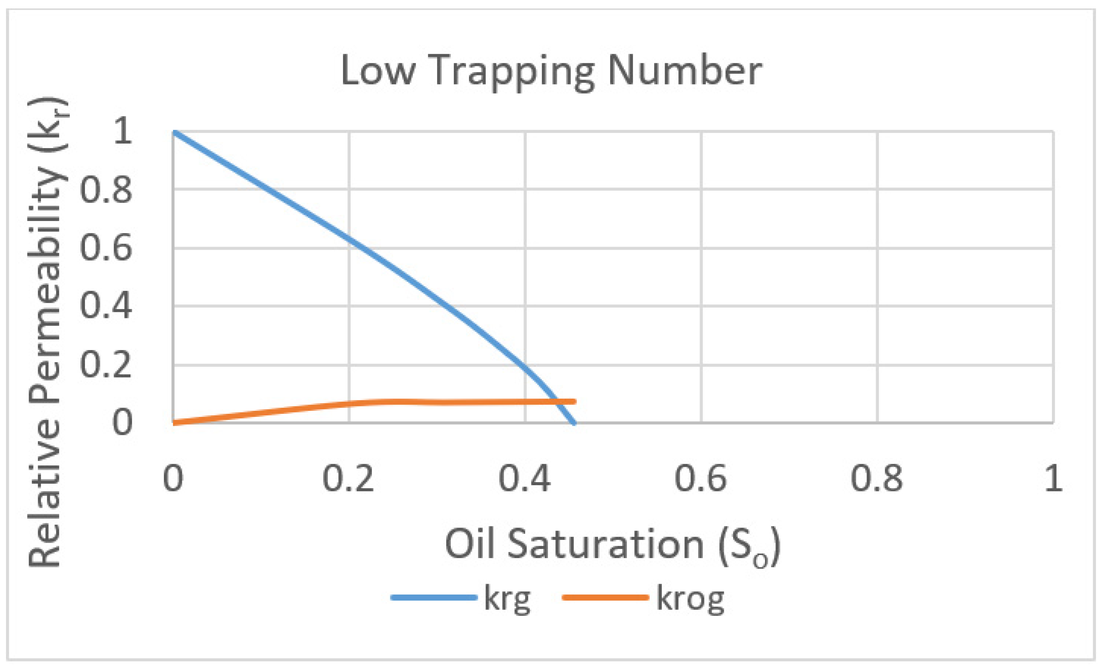
At this stage of the work, we had gathered three relative permeability curves for the final stage of the studies, including the two previously mentioned curves.

The first curve, referred to as the low-trapping-number curve, was presented in the section describing the input data from the GEM simulations. This curve represents the relative permeability curve resulting from the pore network simulations and was adjusted using the Brooks-Corey model. The data for this curve can be found in Table 4, and it is presented in Figure 9.

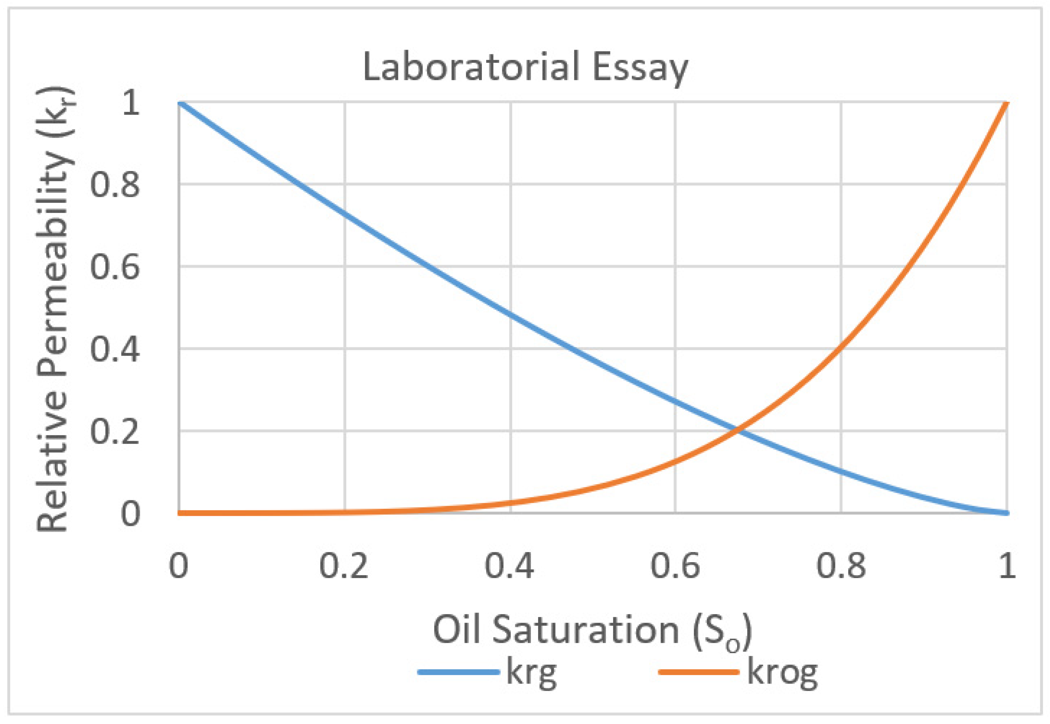
The second curve is called the laboratory test curve, which represents a typical relative permeability curve obtained from a laboratory test. The details of this process were described in the section that presented the inputs for this type of analysis. The laboratory test curve is depicted in Figure 10.

4.5. Field-Scale Simulations

The UNISIM Benchmark reservoir model [25] (Figure 11) was selected for further impact assessments and comparisons using the three available relative permeability curves. This model represents a heterogeneous reservoir with a mesh size of 83 × 45 × 23 gridblocks and dimensions of 105 m × 105 m × 7 m. The porosity and permeability properties in the model were adjusted to match the average values used in this study, which were 155 mD for permeability and 17% for porosity.

The fluid used in the model remained the same as in the previous studies. The field-scale simulation served as a correlation with the last validation scale of the upscaling process and allowed for a comparison of the relative permeability curves. Four wells, called P03, P09, P18, and P43, were positioned along the field. Each well was considered a sink equivalent to the decametric scale simulation, with a gridblock size of 21.2814 m.

4.5.1. Comparison of Productivity

To compare the potential of the producer wells in the field-scale simulation, the productivity index (PI) was calculated for the four wells using the three different relative permeability curves. The PI is a key indicator of a well’s production capacity and can be calculated in two ways: focusing on gas production and focusing on condensate production.

The productivity index is defined as the ratio between the production flow rate and the pressure differential to which the well is subjected. The pressure differential that drives the production of a well is determined by the difference between the static pressure (or average reservoir pressure in the vicinity of the well) and the flow pressure, also known as the bottom-hole pressure.

By calculating the PI for each well under the influence of the different relative permeability curves, we could assess and compare the production potential of the wells in terms of gas and condensate production.

$$PI={\displaystyle \frac{Q}{P_e-P_w}}$$

(16)

where Q = oil flow rate in standard conditions, Pe = average pressure, and Pw = bottom-hole pressure.

The PI calculated according to Equation (16) was used to calculate the oil well productivity index. For gas producer wells, we could use the same equation if the flow considered was the total of the fluids produced under reservoir conditions.

The graphs obtained from this calculation for two of the production wells are shown in Figure 12 and Figure 13. In the graphs, the corresponding legends describe the three evaluated relative permeability curves:

• Lab is the curve from the laboratory experiment (in red);
• Corey_Original is the curve from the pore network simulation adjusted to the Brooks–Corey power law (in green);
• Upscaling is the final curve obtained after the upscaling process with the influence of velocity following Pope et al.’s model (in blue).

When comparing the productivity evolutions using the three relative permeability curves, it is noteworthy that the relative permeability curve resulting from the laboratory test exhibits an optimistic nature. Simulations using this curve come up with higher gas productivity values for a fixed maximum fluid production under reservoir conditions.

4.5.2. Saturation Variation Results

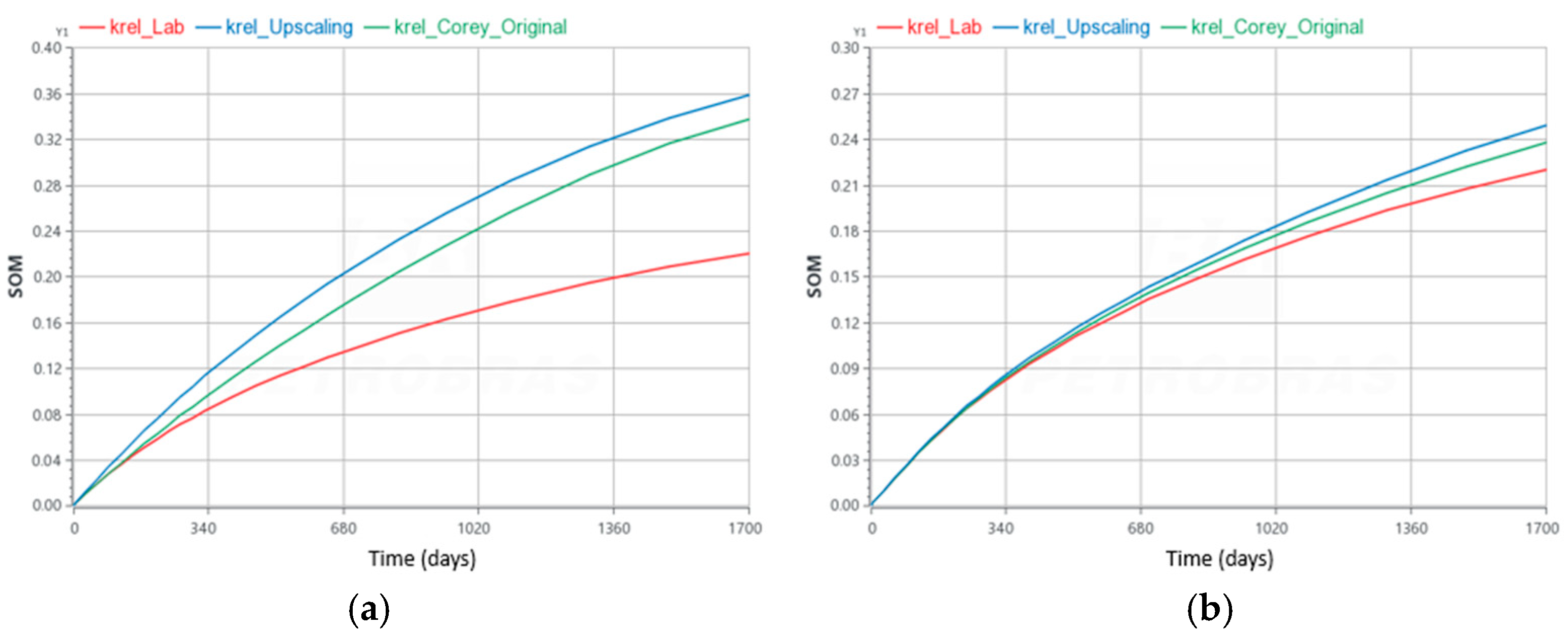
To assess the influence of the three different relative permeability curves on the evolution of condensate saturation over time near the wells, four regions of interest were defined in Figure 14. In this figure, the effective permeability to gas in the presence of condensate at the end of the simulation, which utilized the relative permeability curve resulting from the upscaling process, is depicted. The effective permeability values were calculated using a weighted average based on the porous volume of the defined regions. This allows for a comparison of the condensate saturation evolution in these specific areas under the influence of the different relative permeability curves.

The regions of interest were selected based on a volumetric criterion, encompassing parallelepiped areas composed of gridblocks surrounding the wells. Each region covers three gridblocks in the x-direction, and three gridblocks in the y-direction, including the well-perforated gridblocks, and is located in the lower layers where the highest concentration of condensate occurs after deposition. These regions cover the last five layers of the simulation mesh.

The four regions are assigned as follows: Well03, Well09, Well18, and Well43, corresponding to the gridblocks shown in Figure 14 for wells P03, P09, P18, and P43, respectively.

Figure 15 presents the evolution graphs of the average condensate saturation over the simulation time in the Well09 and Well18 regions. The results were compared for the three simulations using different relative permeability curves, using the same nomenclature as previously mentioned: Lab (curve from the laboratory experiment), Corey_Original (curve from the pore network simulation adjusted to the Brooks–Corey power law), and Upscaling (final curve obtained after the upscaling process with the influence of velocity following Pope et al.’s model). The graphs also include the average oil saturation (SOM).

Table 8. Average effective gas permeability values (mD).

Regions	Start: All	End: krel_Lab	End: krel_Corey_Original	End: krel_Upscaling
Well03	42.13	29.13	19.96	18.70
Well09	74.15	71.56	46.15	45.99
Well18	124.48	119.30	76.60	73.17
Well43	12.01	11.38	6.76	6.55

provides a comparison of the effective permeability to gas in the presence of condensate for the regions of interest in the simulations using the three relative permeability curves. The table shows the average values of permeability in millidarcy (mD) at the beginning and end of the simulations.

Table 9. Percentage reductions in effective gas permeability values.

Regions	krel_Lab	krel_Corey_Original	krel_Upscaling
Well03	30.9%	52.6%	55.6%
Well09	3.5%	37.8%	38.0%
Well18	4.2%	38.5%	41.2%
Well43	5.2%	43.7%	45.5%

displays the percentage reduction in the effective permeability to gas in the presence of condensate between the beginning and end of the simulations for each relative permeability curve used.

These tables and graphs offer insights into the changes in condensate saturation and permeability in the regions of interest under the influence of different relative permeability curves throughout the simulation time.

The graphs consistently show that the condensate saturation evolution curves over time for the simulation using the relative permeability curve from the laboratory test are lower than those using the original Brooks–Corey adjustment, and in turn, the curves using the relative permeability resulting from the scaling process are higher than both.

Based on the property presented in Figure 14, the average effective gas permeability values for the chosen regions take the following ascending order: Well43, Well03, Well09, and Well18. This order remains consistent throughout the simulation, with all four regions near the wells showing reductions in effective gas permeability using any of the three relative permeability curves.

The largest percentage reductions in effective gas permeability in the presence of condensate occur in the simulation using the relative permeability curve resulting from the upscaling process. Slightly lower reductions are observed in the simulation using the initial relative permeability curve with Brooks–Corey adjustment. The simulation using the relative permeability curve from the laboratory test shows the lowest percentage reductions in effective gas permeability.

Based on these observations, it is evident that the relative permeability curve from the laboratory test tends to underestimate condensate deposition in regions near the wells, particularly in areas of greater depletion. This curve consistently exhibits lower condensate saturation values compared to the other two relative permeability curves used in this study.

Additionally, the curve referred to as krel_Lab is more optimistic in terms of representing the reduction in effective gas permeability in the presence of condensate. This is because, when comparing the beginning and end of the simulation, it suggests that gas can still flow reasonably well, despite potentially having its flow capacity reduced by around 50% under the considered simulation time and reservoir conditions. In contrast, the krel_Corey_Original and krel_Upscaling curves provide a more realistic representation of the phenomenon, with higher condensate saturation values and greater percentage reductions in effective gas permeability throughout the simulation.

Overall, the comparison between the krel_Corey_Original and krel_Upscaling curves indicates that the krel_Upscaling curve better represents the phenomenon in the selected regions. This is supported by higher condensate saturation values and greater percentage reductions in effective gas permeability observed in the simulation using the krel_Upscaling curve.

5. Conclusions

This article has introduced a methodology for upscaling gas–oil relative permeability from a digital petrophysics scale to field-scale simulations. The studies conducted validate the ability to reproduce fine-scaled simulations in commercial simulators and bring forth the following main conclusions:

• Simulations using the gas–oil relative permeability curve obtained from laboratory tests showed different results compared to those obtained through the upscaling process. The upscaling process represents the condensate as a more mobile fluid than the mobility that it would have if the initial relative permeability curve had been considered. Hence, our upscaling strategy could represent the condensate mobility accurately, resulting in less damage to the gas phase due to the reduced accumulation of condensate in the reservoir. These findings indicate that the proposed methodology provides a more accurate representation of the influence of condensation on well productivity.
• When evaluating well productivity in detail, no significant differences were observed between using the original gas–oil relative permeability curve and the upscaled result. The main objective of upscaling processes is to capture the influence of scale changes, and while some impact was observed in this study, it was relatively small.
• However, when analyzing the time evolution of condensate saturation in selected regions near well perforations, a clearer distinction was observed among the three gas–oil relative permeability curves. The gas–oil relative permeability curve obtained from laboratory tests showed the lowest condensate saturation values, followed by the curve adjusted to data from the pore network simulation, and the highest saturation values were observed in the curve resulting from the upscaling process.
• The incorporation of the trapping number model, which considers the influence of interfacial tension and flow velocity on the gas–oil relative permeability curve used in numerical simulations, can offer a valuable tool for capturing the compositional changes occurring in regions near producer wells. Combining this model with the proposed upscaling methodology applied to pore network simulation results can enhance the representativeness of field-scale numerical simulations for reservoir engineers.

Overall, this research highlights the significance of incorporating condensation effects and upscaling in gas–oil relative permeability modeling. It offers meaningful insights for reservoir engineering applications, even though it lacks field data to support and expand the proposed method. This study emphasizes the impact of scale on relative permeability when condensate develops in porous media and how this can be extended to field-scale grids. Moving forward, it is recommended that efforts should be made to validate the approach by applying it to a real-world scenario using a history-matching workflow.