Atmospheric Correction of Thermal Infrared Landsat Images Using High-Resolution Vertical Profiles Simulated by WRF Model ^†

Abstract

Atmospheric profiles are key inputs in correcting the atmospheric effects of thermal infrared (TIR) remote sensing data for estimating land surface temperature (LST). This study is a first insight into the feasibility of using the weather research and forecasting (WRF) model to provide high-resolution vertical profiles for LST retrieval. WRF numerical simulations were performed to downscaling NCEP climate forecast system version 2 (CFSv2) reanalysis profiles, using two nested grids with horizontal resolutions of 12 km (G12) and 3 km (G03). We investigated the use of these profiles in the atmospheric correction of TIR data applying the radiative transfer equation (RTE) inversion single-channel approach. The MODerate resolution atmospheric TRANsmission (MODTRAN) model and Landsat 8 TIRS10 (10.6–11.2 µm) band were taken for the method application. The accuracy evaluation was performed using in situ radiosondes in Southern Brazil. We included in the comparative analysis the atmospheric correction parameter calculator (ACPC; NASA) web tool and profiles directly from the NCEP CFSv2 reanalysis. The atmospheric correction parameters from ACPC, followed by CFSv2, had better agreement with the ones calculated using in situ radiosondes. When applied into the RTE to retrieve LST, the best results (RMSE) were, in descending order: CSFv2 (0.55 K), ACPC (0.56 K), WRF G12 (0.79 K), and WRF G03 (0.82 K). The findings suggest that increasing the horizontal resolution of reanalysis profiles does not particularly improve the accuracy of RTE-based LST retrieval. However, the WRF results are yet satisfactory and promising, encouraging further assessments. We endorse the use of the well-known ACPC and also recommend the NCEP CFSv2 reanalysis profiles for TIR remote sensing atmospheric correction and LST single-channel retrieval.

1. Introduction

Land surface temperature (LST) is a key parameter in a wide variety of environmental applications. It is closely connected and plays an important role in Earth’s surface-atmosphere interactions at both local and global scales [1,2,3,4]. Thermal infrared (TIR) remote sensing is an outstanding way of obtaining the LST at regional and global scales [5,6,7]. Nevertheless, the spectral radiation measured by TIR sensors onboard satellites is determined not only by the surface parameters (emissivity and temperature) but also by the atmosphere effects (mainly due to water vapor) [6,8]. These atmospheric perturbations must be compensated for the correct use of TIR remote sensing data [4,9]; in general terms, the conversion of the top of the atmosphere (TOA) signal to the ground level. This process is named atmospheric correction (AC) and neglecting it results in systematic errors in the LST estimation for any atmosphere [8,10].

The physics-based radiative transfer equation (RTE) method [11] is one of the most applied methodologies to AC and LST retrieval. It consists of a direct inversion of the RTE for a particular channel and can provide theoretically accurate LST retrieval [6]. The RTE approach requires vertical atmospheric profiles. This information is introduced into a radiative transfer model (RTM) to calculate the three atmospheric parameters required for AC: atmospheric transmittance, upwelling atmospheric radiance, and downwelling atmospheric radiance [8,12]. In situ radiosonde profiles launched simultaneously with the satellite overpass are ideal for AC [5,13]. Nevertheless, this kind of profile is unavailable under the most realistic conditions [5,14,15] and so its use is suitable only for particular local studies and validations at specific sites [7,14].

To surpass the radiosondes spatiotemporal limitation, atmospheric profile products derived from global reanalysis data have been used as a practical alternative in TIR atmospheric correction, resulting in LSTs with acceptable accuracy [9,16,17,18,19,20]. Nonetheless, these profiles also have disadvantages. The spatial resolution is considered low (several degrees, varying for each product). The accuracy is usually poor for regions with less coverage of permanent observatories, such as the oceans and many Southern Hemisphere countries [21,22,23]. Modern numerical weather prediction (NWP) models benefit from computing performance and physical processes parameterization to downscaling the reanalysis data [24]. Mesoscale atmospheric models use global (re)analysis as initial and boundary conditions for local applications [24,25]. Lee et al. (2020) [26] used high-resolution Korean NWP models as input atmospheric data for AC and sea surface temperature estimation with VIIRS sensor bands.

The weather research and forecasting (WRF) model [27] is an atmospheric modeling system designed for both research and NWP. It is the world’s most used mesoscale model and provides capabilities for a range of applications in terrestrial systems. The WRF model has been widely employed for estimating high-resolution meteorological data [28,29,30]. It is all-important to assess the reasonableness of using the WRF model to generate high-resolution atmospheric profiles to perform, in conjunction with an RTM, more accurate AC/LST retrieval. Moreover, the vast majority of studies that evaluated different profile sources for LST retrieval were carried out over Asia and Europe. To the best of our knowledge, no paper has conducted such an assessment in South America. There is also a need for studies using newer and finer reanalysis profiles (e.g., ERA5 and NCEP CFSv2) for AC and LST estimation [19,31].

This paper conducts simulations with the WRF Model using NCEP CFSv2 reanalysis data as initial and boundary conditions. It aims to generate high-resolution vertical profiles, improving the spatial and temporal resolutions of the global reanalysis. Moreover, it aims to analyze the utility of these profiles in the atmospheric correction of TIR images and LST retrieval, through an RTE-based algorithm using the MODTRAN radiative transfer model and Landsat 8 TIRS band 10. The accuracy assessment was performed using local radiosonde observation in Southern Brazil. The well-established atmospheric correction parameter calculator (ACPC; NASA) web tool [10,12] and profiles extracted directly from the NCEP CFSv2 reanalysis were included in the comparative analysis.

2. Data and Methods

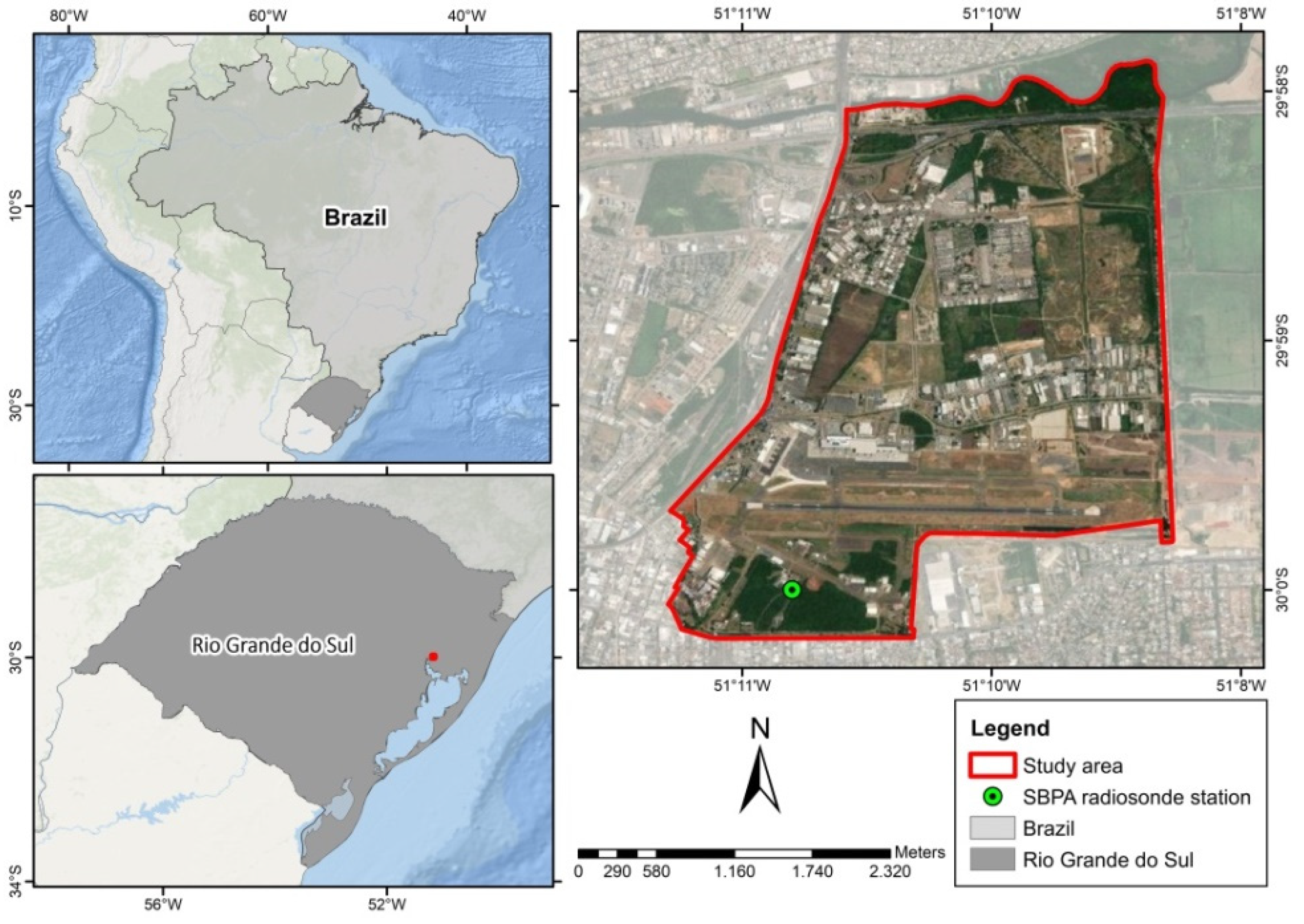
2.1. Study Area and In Situ Radiosonde Data

The Porto Alegre International Airport (SBPA), Rio Grande do Sul State, Brazil was selected as the study area. The SBPA includes a radiosonde station, which makes this site useful for studies that aim to validate atmospheric profiles. The selected area covers the official limits of the Anchieta district, with an area of around 9.2 km² (Figure 1). The SBPA station is located at 30.00° S and 51.18° W, 3.0 m above mean sea level. Radiosondes are launched twice a day, at 00:00 and 12:00 UTC. We used the 12:00 UTC radiosonde profiles, as this is the closest to the Landsat 8 crossing time over the study site (~13 UTC). This dataset allows characterizing the vertical structure of the atmosphere with profiles of air temperature, pressure, humidity with up to 99 vertical levels. The radiosonde observations, as well as the parameters calculated from them, were used as the ground truth for the assessments.

2.2. Satellite and Reanalysis Data

Landsat 8 carries a two-sensor payload: the operational land imager (OLI) that has nine reflective bands and the thermal infrared sensor (TIRS) with two bands in the TIR region. We acquired all Landsat 8 images (Collection 1) available under daily clear-sky conditions over the study site (Path-Row 221-81) from 2013 to 2019, which resulted in a total of 27 scenes, henceforward refer as case days 1–27. The full swath Landsat data were subset to a 10,184 pixels region covering the study area of Figure 1. The TIRS band 10 (10.60–11.19 µm) is used for RTE-based LST retrieval and OLI bands 4—red (0.64–0.67 µm) and 5—near-infrared (NIR) (0.85–0.88 µm) for land surface emissivity estimation.

Additionally, we used the NCEP climate forecast system version 2 (CFSv2) [32] reanalysis data from the 6-hourly product as initial and boundary conditions for the WRF simulations. NCEP CFSv2 reanalysis data is produced using the NCEP global forecasting system (GFS) atmospheric model and the grid point statistical interpolation (GSI) analysis system with three-dimensional variational data assimilation (3D-Var). It is arranged in grids with a horizontal resolution of 0.5° × 0.5° in 37 vertical (pressure) levels (1000–1 mbar), and of 0.205° for surface parameters. Besides, profiles retrieved directly from NCEP CFSv2 were included in the analysis, to assess the WRF model horizontal resolution downscaling performance. These profiles were extracted from the grid point closest to the SBPA station.

2.3. WRF Model Configuration

The WRF Model version 4.1.2 with the advanced research WRF (ARW) dynamical solver [27] was used to perform high-resolution numerical simulations. We configured the WRF domains with two nested grids, in one-way mode, centered at SBPA station, with horizontal resolutions of 12 km (G12) and 3 km (G03) (4:1 parent grid ratio), and 33 sigma vertical levels with 50 hPa top pressure value. The WRF configurations used are summarized in

Table 1. Overview of WRF model setting.

WRF Model Configuration
Version	4.1.2
Dynamical solver	ARW
Boundary conditions	NCEP CFSv2
Map projection	Lambert
Grid size	Domain 1: (119 × 116) × 33 Domain 2: (169 × 165) × 33
Horizontal resolution	Domain 1: 12 km Domain 2: 3 km
Nesting	One-way
Time step	72s
Static geographical data	USGS
Cloud microphysics	Purdue Lin
Planetary boundary layer (PBL)	Yonsei University (YSU)
Cumulus	Betts–Miller–Janjic (BMJ) 1
Shortwave radiation	Dudhia
Longwave radiation	Rapid radiative transfer model (RRTM)
Land-surface model (LSM)	Unified NOAH
Surface-layer	Revised MM5

¹ Domain 1 only.

. The physics parameterizations chosen for our simulations are based on Santos and Nascimento (2016) [33] for the same station. The model was run in the below settings for each case day. The profiles resulted from simulations were retrieved from the model grid point closest to the SBPA station We conduct simulations of 24 h duration and the results were extracted at 12:00 UTC, to match with the local radiosonde observations. Thus, the first 12 h of the simulation was considered for a spin up time.

2.4. Land Surface Emissivity Estimation

Land surface emissivity (LSE) is one of the key parameters to retrieve LST from remote sensing data [34,35]. Among the methods for LSE retrieval from space, normalized difference vegetation index (NDVI)-based ones are operational and the most applied, with satisfactory results [36,37,38,39]. Sekertekin and Bonafoni (2020a, 2020b) [40,41] examined the influence of six NDVI-based LSE models on the performance of LST retrieval. Based on their results, we used the NDVI threshold method (NDVI^THM) proposed by Sobrino et al. (2008) [36].

The NDVI is obtained from Equation (1):

$$\mathrm{NDVI}=\frac{{\mathsf{\rho }}_{\mathrm{NIR}}-{\mathsf{\rho }}_{\mathrm{R}}}{{\mathsf{\rho }}_{\mathrm{NIR}}+{\mathsf{\rho }}_{\mathrm{R}}}$$

(1)

where ${\mathsf{\rho }}_{\mathrm{NIR}}$ and and ${\mathsf{\rho }}_{\mathrm{R}}$ are the reflectances of NIR and red bands, respectively. From NDVI, it is possible to calculate the fractional vegetation cover (${\mathrm{P}}_{\mathrm{V}}$) from Equation (2) [42]. The ${\mathrm{P}}_{\mathrm{V}}$ is an important factor in the LSE estimation.

$${\mathrm{P}}_{\mathrm{V}}={\left[\frac{\mathrm{NDVI}-{\mathrm{NDVI}}_{\min }}{{\mathrm{NDVI}}_{\max }-{\mathrm{NDVI}}_{\min }}\right]}^2$$

(2)

where ${\mathrm{NDVI}}_{\min }$ = 0.2 and ${\mathrm{NDVI}}_{\max }$ = 0.5 in a global context [13,36].

The NDVI^THM estimates LSE considering three different cases as presented in Equation (3), for Landsat 8 [40]. For NDVI < 0.2, the pixel is considered as bare soil, and the emissivity is calculated using the reflectance of the red band. In the second case (0.2 ≤ NDVI ≤ 0.5), the pixel is considered composed of a mixture of bare soil and vegetation and the LSE depends on the ${\mathrm{P}}_{\mathrm{V}}$ value. The pixels with NDVI values higher than 0.5 are considered as fully vegetated areas and the emissivity is assumed as 0.99.

$$\mathsf{\epsilon }=\{\begin{array}{c}0.979-0.035{\mathsf{\rho }}_{\mathrm{R}}\\ 0.004{\mathrm{P}}_{\mathrm{V}}+0.986\\ 0.99\end{array}\begin{array}{c}\mathrm{NDVI}<0.2\\ 0.2\le \mathrm{NDVI}\le 0.5\\ \mathrm{NDVI}>0.5\end{array}$$

(3)

where $\mathsf{\epsilon }$ is the Land Surface Emissivity (LSE).

2.5. Atmospheric Correction and LST Retrieval

2.5.1. Atmospheric Parameters Calculation with MODTRAN and ACPC

The present study used the MODTRAN (MODerate resolution atmospheric TRANsmission) 4 v3r1 [43] to estimate the three atmospheric correction parameters (i.e., atmospheric transmittance, upwelling atmospheric radiance, and downwelling atmospheric radiance) in the Landsat TIR spectrum. We introduced into the MODTRAN as input vertical profiles of pressure, air temperature, and relative humidity from: (i) SBPA radiosonde; (ii) NCEP CFSv2 reanalysis; (iii) WRF G12; and (iv) WRF G03.

The methodology of Barsi et al. (2003) [12], to fulfill the profiles, was adopted. To predict space-reaching atmospheric parameters, the MODTRAN requires atmospheric profiles reaching “space”, or 100 km above sea level. Since the radiosondes and NCEP CFSv2 are from the surface to about 30 and 50 km, respectively, the upper atmosphere layers (to 100 km) are extracted from the MODTRAN standard atmospheres and pasted onto our site-specific profiles. We take on the standard mid-latitude summer profile for case days in hot seasons (spring and summer) and the mid-latitude winter profile for those in cold seasons (autumn and winter). This results in surface-to-space vertical profiles of air temperature, pressure, and water vapor. These completed profiles are those that are inserted into a MODTRAN input file and then processed [10,12].

Moreover, we include in the comparative analysis the atmospheric parameters estimated by the well-known atmospheric correction parameter calculator (ACPC; NASA) web tool [10,12]. The ACPC uses NCEP reanalysis profiles (1° × 1° horizontal resolution and 28 vertical levels), MODTRAN code, and a suite of integration algorithms to directly provide the AC parameters for a particular date, time, and location inputted. The option of using the atmospheric profile from the closest integer coordinate to the inputted location (SBPA station) was set. The mid-latitude standard upper profiles varied according to the season of each case day.

2.5.2. Radiative Transfer Equation (RTE) Based LST Retrieval Method

The inverse solution of RTE [11] is a direct and a priori the most appropriate procedure for LST retrieval using a single TIR band [44]. The RTE applied to a particular TIR band/wavelength (λ) can be simplified and given by:

$${\mathrm{L}}_{\mathsf{\lambda }}^{\mathrm{sen}}=\left[{\mathsf{\epsilon }}_{\mathsf{\lambda }}{\mathrm{B}}_{\mathsf{\lambda }}\left({\mathrm{T}}_{\mathrm{s}}\right)+\left(1-{\mathsf{\epsilon }}_{\mathsf{\lambda }}\right){\mathrm{L}}_{\mathsf{\lambda }}^{\downarrow }\right]{\mathsf{\tau }}_{\mathsf{\lambda }}+{\mathrm{L}}_{\mathsf{\lambda }}^{\uparrow }$$

(4)

where ${\mathrm{L}}_{\mathsf{\lambda }}^{\mathrm{sen}}$ (W·m⁻²·sr⁻¹·µm⁻¹) is the at-sensor (TOA) spectral radiance of the corresponding TIR band (in this paper, TIRS10), ${\mathsf{\epsilon }}_{\mathsf{\lambda }}$ refers to the LSE (dimensionless), ${\mathrm{B}}_{\mathsf{\lambda }}$ (W·m⁻²·sr⁻¹·µm⁻¹) is the blackbody radiance, ${\mathrm{T}}_s$ (Kelvin) represents the LST, ${\mathrm{L}}_{\mathsf{\lambda }}^{\downarrow }$, and ${\mathrm{L}}_{\mathsf{\lambda }}^{\uparrow }$ (W·m⁻²·sr⁻¹·µm⁻¹) refer to the downwelling and upwelling radiances, respectively, and ${\mathsf{\tau }}_{\mathsf{\lambda }}$ is the atmospheric transmittance (dimensionless). So, the emitted radiance for a black body at a temperature ${\mathrm{T}}_{\mathrm{s}}$ is given by the inversion of Equation (4):

$${\mathrm{B}}_{\mathsf{\lambda }}\left({\mathrm{T}}_{\mathrm{s}}\right)=\frac{{\mathrm{L}}_{\mathsf{\lambda }}^{\mathrm{sen}}-{\mathrm{L}}_{\mathsf{\lambda }}^{\uparrow }-\mathsf{\tau }\left(1-{\mathsf{\epsilon }}_{\mathsf{\lambda }}\right){\mathrm{L}}_{\mathsf{\lambda }}^{\downarrow }}{{\mathsf{\tau }}_{\mathsf{\lambda }}{\mathsf{\epsilon }}_{\mathsf{\lambda }}}$$

(5)

the ${\mathrm{T}}_{\mathrm{s}}$ is calculated by inverting Planck’s law in Equation (5) and the LST (${\mathrm{T}}_{\mathrm{s}}$) from Landsat 8 TIRS10 is estimated as:

$$\mathrm{LST}=\frac{{\mathrm{K}}_2}{\ln \left(\frac{{\mathrm{K}}_1}{\frac{{\mathrm{L}}_{\mathsf{\lambda }}^{\mathrm{sen}}-{\mathrm{L}}_{\mathsf{\lambda }}^{\uparrow }-{\mathsf{\tau }}_{\mathsf{\lambda }}\left(1-{\mathsf{\epsilon }}_{\mathsf{\lambda }}\right){\mathrm{L}}_{\mathsf{\lambda }}^{\downarrow }}{{\mathsf{\tau }}_{\mathsf{\lambda }}{\mathsf{\epsilon }}_{\mathsf{\lambda }}}}+1\right)}$$

(6)

where ${\mathrm{K}}_1$ and ${\mathrm{K}}_2$ refers to calibration constants, whose values for the Landsat 8 TIRS10 are 774.89 W·m⁻²·sr⁻¹·µm⁻¹ and 1321.08 K, respectively [45]. Henceforth, the spectral notation (λ) will be omitted, since here only a single TIR band is used.

The aforementioned procedure was applied with τ, ${\mathrm{L}}^{\uparrow }$, and ${\mathrm{L}}^{\downarrow }$ calculated using profiles from: (i) SBPA local radiosonde; (ii) NCEP CFSv2 reanalysis; (iii) WRF G12; (iv) WRF G03; (v) ACPC.

2.6. Metrics for Performance Evaluation

To evaluate the performance of the WRF model and other profiles we take into account the atmospheric parameters and LST images. The SBPA radiosondes are the available in situ observations. Hence, the AC parameters and LSTs calculated using SBPA profiles are considered our references. To perform the comparative assessment, Pearson’s correlation coefficient (R), bias (mean error), mean absolute error (MAE), and root mean square error (RMSE) were used as statistical criteria. These metrics are widely employed to evaluate and compare models.

3. Results and Discussion

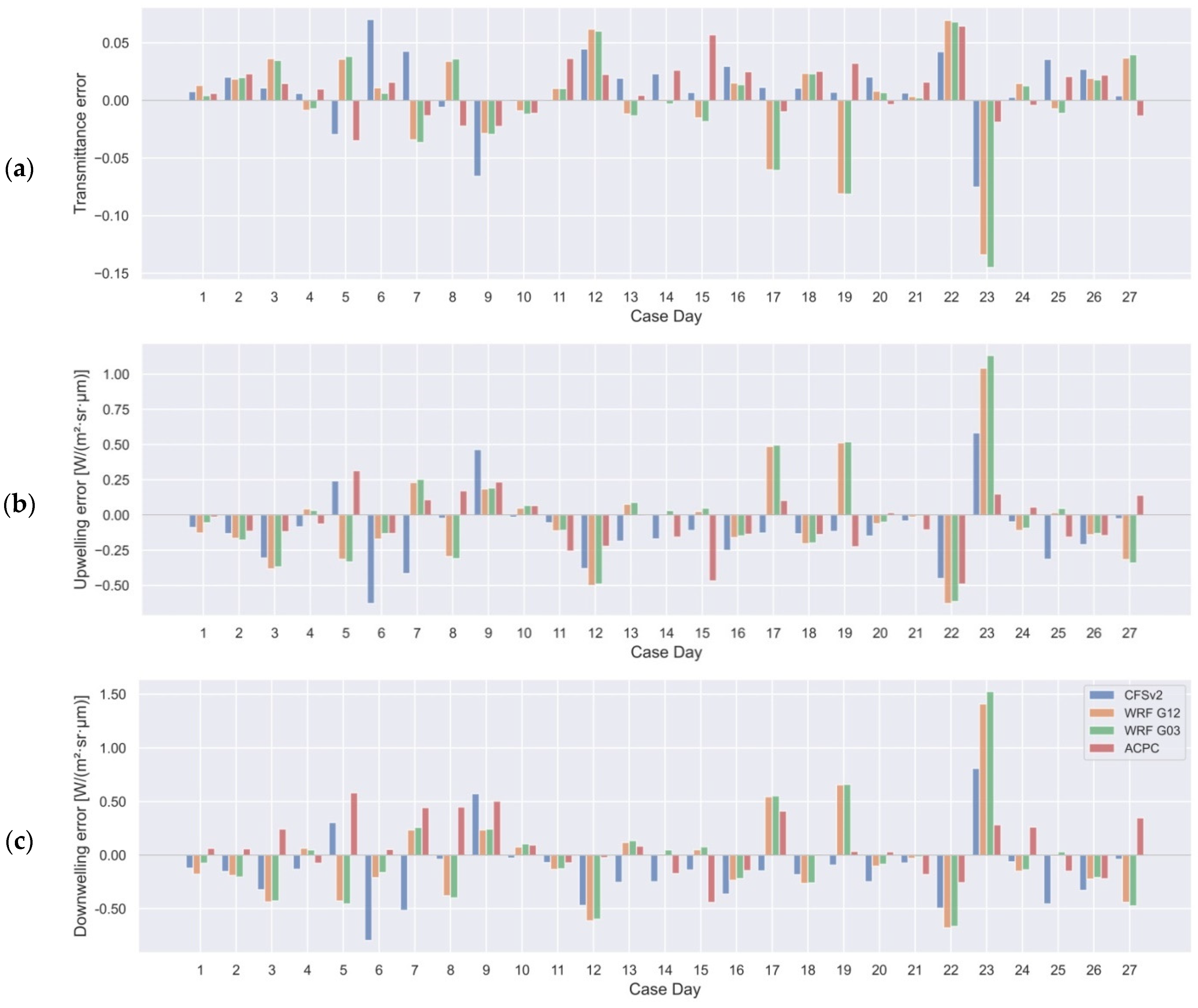
3.1. Evaluation of Atmospheric Parameters

The AC parameters (τ, ${\mathrm{L}}^{\uparrow }$, and ${\mathrm{L}}^{\downarrow }$) calculated with the different sources of estimated vertical profiles (CFSv2, WRF G12, WRF G03, and ACPC) were compared against those using observational SBPA radiosondes. In

Table 2. Statistical metrics of atmospheric parameters estimated from different atmospheric profiles. Bias, MAE, and RMSE are in the parameter of interest units, i.e., W·m⁻²·sr⁻¹·µm⁻¹ for atmospheric radiances and the transmittance is dimensionless.

		CFSv2	WRF G12	WRF G03	ACPC
Transmittance	R	0.96	0.93	0.93	0.97
	bias	0.01	~0.00	~0.00	0.01
	MAE	0.02	0.03	0.03	0.02
	RMSE	0.03	0.04	0.04	0.03
Upwelling	R	0.97	0.94	0.94	0.98
	bias	−0.12	−0.04	−0.02	−0.06
	MAE	0.21	0.24	0.24	0.16
	RMSE	0.27	0.33	0.34	0.20
Downwelling	R	0.97	0.95	0.95	0.98
	bias	−0.15	−0.05	−0.03	0.08
	MAE	0.28	0.30	0.30	0.21
	RMSE	0.35	0.42	0.43	0.27

, the accuracy of atmospheric parameters estimations is presented. All the profile sources provide AC parameters with high correlation coefficients (all greater than 0.9) concerning the reference (SBPA). The R values of ACPC, followed by CFSv2, are slightly better. There is a general but small tendency of overestimating the transmittance values. On the other hand, the atmospheric radiances tend to be underestimated, except for ACPC downwelling. The smallest biases were from the WRF for all three parameters. The largest ones were from CFSv2. Concerning MAE and RMSE, the best results were from ACPC followed by CFSv2.

The higher negative bias of the atmospheric radiances with NCEP CFSv2 in our finds may be due to that these reanalysis profiles have the lowest level at 1000 hPa, which means around 60–250 m for SBPA station in analyzed case days. So the lowest layer of the atmosphere (which typically presents the largest water vapor content and warmest temperature) is neglected in these profiles [5,14]. We had tried to reduce this limitation by downscaling the CFSv2 reanalysis profiles with the WRF model. The WRF profiles bring the first level at around 1 m above the surface.

Our RMSE range is in agreement with those found for reanalysis profiles (eight different products) in Meng and Cheng (2018) [5] for the three parameters. The authors analyzed 30,715 atmospheric profiles in 163 stations around the globe. The RMSE values of Yang et al. (2020) [46] were overall slightly lower than ours. Their assessment included seven profiles sources over Europe.

The errors in the estimation of atmospheric parameters for each case day are shown in Figure 2. It shows that despite ACPC presented the best overall metrics, none of the profile sources outperforms in all cases. For instance, in 8 of the 27 case days, one of the WRF profiles had the best results in calculating the downwelling radiance. In case day 23, the WRF model produced the largest errors, whereas in cases such as 26 the model successfully reduced the largest error of the driving reanalysis data.

On the whole, ACPC obtained better results than the other profiles for all three atmospheric parameters. Then, comes the CFSv2 reanalysis. Table 2 points out that no significant statistical differences were found between the parameters’ accuracies from the WRF grids G12 and G03. It suggests that computation costs can be saved by using profiles from a WRF domain with coarse horizontal resolution. Despite other aims, scholars have already reported this kind of result with WRF model grids [24,47,48,49,50].

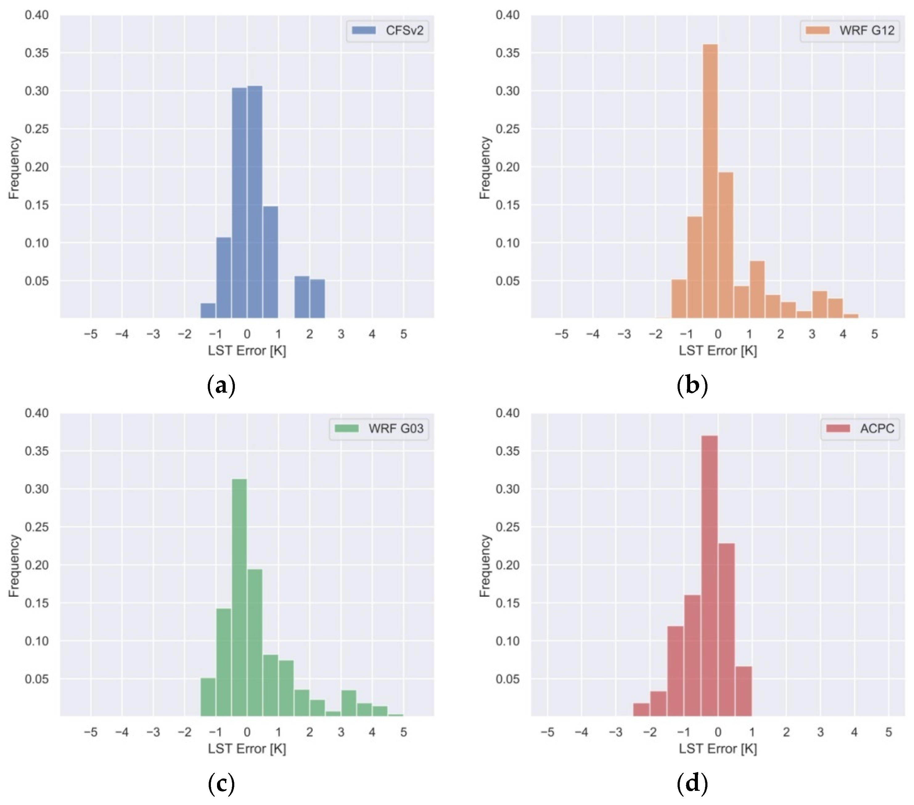
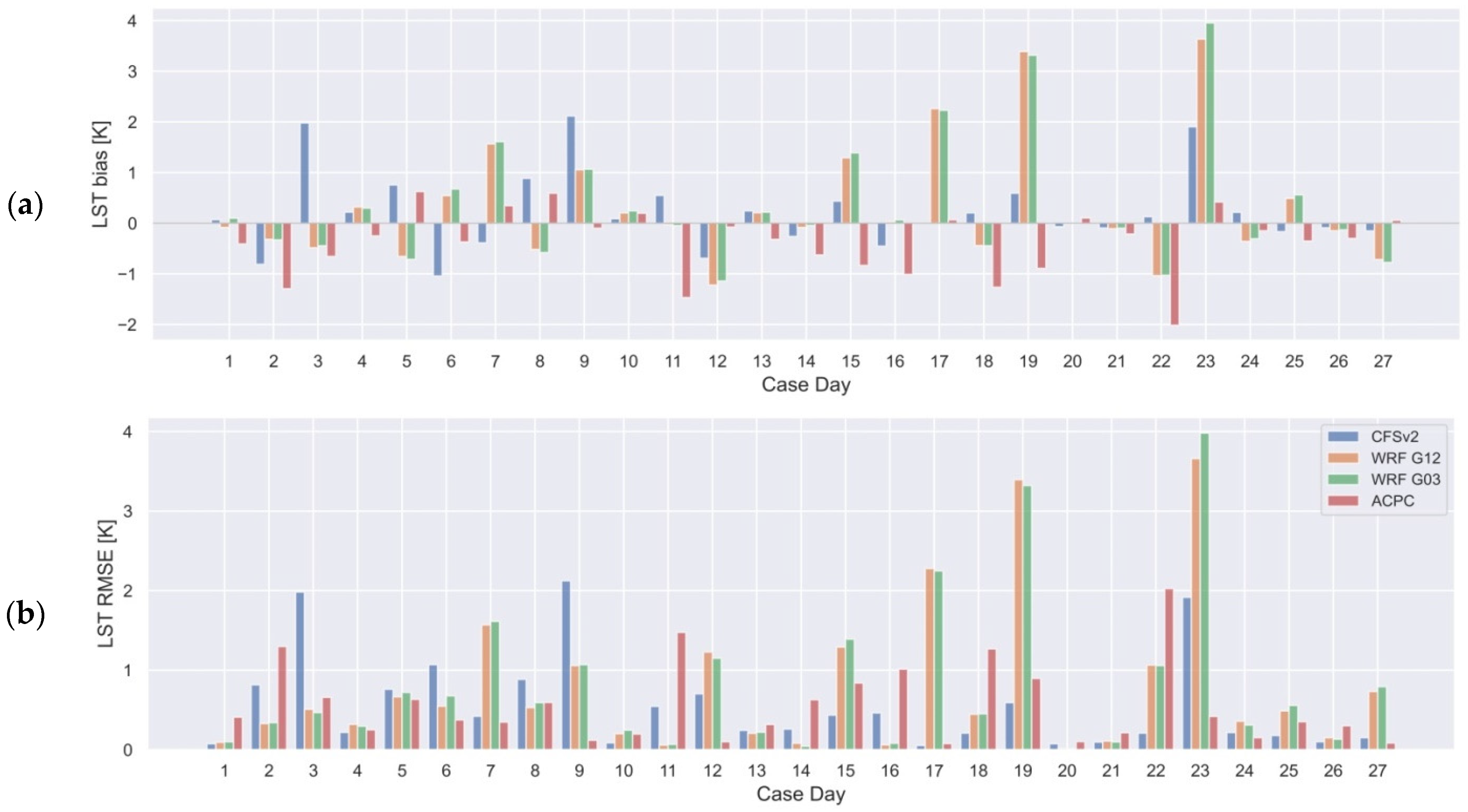
3.2. Application to RTE-Based LST Retrieval

To further assess the different atmospheric profiles, the retrieved LSTs by RTE inversion with atmospheric parameters, Landsat 8 TIRS10 radiance, and NDVI^THM emissivity were intercompared. Once more, the LST images that used SBPA profiles were assumed as reference data. Except for the atmospheric parameters calculated from the different profile sources, the other variables in Equation (6) were the same for each pixel of the scenes. Therefore, the differences in LST values are due to the discrepancies among the profiles [46].

Histograms of LST errors take in all the 10,184 pixels in the study area of the 27 case days are shown in Figure 3. These represent the frequency distribution of the errors in the retrieval of LST using the different atmospheric profile sources. For all profiles, more than 50% of the errors are of ±1 K. Yang et al. (2020) [46] also found most of the LST differences in this range, using seven different reanalysis and satellite-derived profiles. The histograms in Figure 3b and Figure 4c indicate that WRF profiles tend to overestimate the LST. Whereas ACPC tends to underestimate it (Figure 3d). Using WRF profiles, LST errors can reach more than 4 K, although in a very small number of cases. For ACPC and both WRF grids, the error range that occurs most often is between 0 and −1 K. The distribution of CFSv2 LST errors is more symmetrical than in the other profiles.

Table 3. Statistical metrics of land surface temperature (LST) retrieved using atmospheric parameters from different profile sources. The LST values calculated with SBPA parameters were considered as references.

		CFSv2	WRF G12	WRF G03	ACPC
LST [K]	R	0.99	0.99	0.99	0.99
	bias	0.23	0.32	0.36	−0.38
	MAE	0.54	0.79	0.81	0.56
	RMSE	0.55	0.79	0.82	0.56

summarizes the metrics of the LST retrieval comparative analysis. Overall, the LST values of the four profile sources analyzed in this study were found in good agreement with the reference. All of them showed a very strong correlation and relatively low bias, MAE, and RMSE values. CFSv2, WRF G12, and WRF G03 presented an average positive bias and ACPC a negative one. This corroborates with the histogram analysis in Figure 3. The mean error criteria (MAE and RMSE) indicate that the profiles with the best performance in the RTE-based LST retrieval are, in descending order: CSFv2, ACPC, WRF G12, and WRF G03. The differences between CFSv2 and ACPC overall MAE and RMSE values were very small. The same for WRF G12 and G03.

Comparing with previous studies that evaluated the application of different atmospheric profiles in the LST retrieval, Meng and Cheng (2018) [5] reported overall LST RMSE values higher than ours using the Landsat 8 TIRS10 band and eight different reanalysis profile sources analyzed around the globe. All their eight average RMSEs were larger than 1 K. They also indicated an average tendency to overestimate the LST. In a study by Yang et al. (2020) [46], RMSEs ranged between 0.6–1 K comparing LST retrieved from Landsat 8 TIRS10 over Europe. Calculating LST from three MODIS thermal bands, Pérez-Planells et al. (2015) [51] showed RMSEs between 0.6 and 0.9 K using ACPC/NCEP and between 1.3 and 3 K for MOD07 profiles, depending on the band and the altitude of the study sites in Spain.

Figure 4 displays the distribution of LST bias and RMSE along the case days. Figure 4a evidences the ACPC and WRF settings average tendency of under and overestimate the LST, respectively. We found better RMSE values using CFSv2 in 11 of the 27 case days, and in 8 using ACPC. Although the metrics of mean errors are greater for WRF profiles, in 11 case days the model improves the results of the reanalysis. Besides, the finer grid (G03) succeeded in downscaling the G12 11 times. The fact is that the largest errors were achieved when using the WRF model (e.g., case days 23, 19, and 17), and it contributes to the higher overall RMSE values. In general, the days with larger errors in atmospheric parameters (Figure 2) are the days with larger LST RMSEs, as evinces case 23. Conversely, in case 22, the errors in atmospheric parameters using ACPC are less than those using WRF profiles, but the highest LST RMSE on this day is with ACPC. Jiménez-Muñoz et al. (2010) [8] advocate that cases like this may be explained due to compensation among AC parameters errors; for instance, a significant positive difference in transmittance and significant but negative differences in the atmospheric radiances.

In summary, the essay of downscaling the horizontal resolution of reanalysis data from 0.5° (~56 km) to 12 km and so to 3 km, aiming to reduce errors in the calculation of atmospheric parameters and hence in LST retrieval, did not perform as theoretically expected. With WRF simulations, we also improved the vertical resolution in the lowest atmospheric levels. However, no significant improvement was found using the WRF profiles in the AC. In some cases, using a finer grid resolution profile resulted in greater uncertainties in atmospheric parameters and LST estimation. Rosas et al. (2017) [7] reported that the higher vertical resolution of NCEP and ECMWF profiles in their study did not seem to play a significant role in the atmospheric correction. Even if, naturally, data with higher resolution tend to better represent the atmosphere parameters, it is not a strictly direct relationship [5,46]. Furthermore, the ACPC that uses profiles with 1° × 1° (~100 km) horizontal resolution showed good results. Although these profiles have a coarser horizontal resolution, previous studies have been finding satisfactory results using the ACPC, even surpassing other methods [8,16,38,52,53]. It is important to note that in this study the WRF resulting profiles were extracted at 12 UTC to match with the available radiosonde data. Nevertheless, it could be set for the exact time of the satellite overpass. In ACPC and, in general, for reanalysis profiles, this time synchronization is done through linear interpolation. Which may not be the most appropriate strategy for sampling weather fronts and diurnal heating cycles [5,10,12].

4. Conclusions

Vertical atmospheric profiles are key inputs in the atmospheric correction for estimating LST using the RTE inversion single-channel approach. This study evaluated the use of the WRF numerical model to simulate high-resolution profiles improving horizontal, temporal, and vertical resolutions of NCEP CFSv2 reanalysis data. The obtained results showed that the ACPC provided atmospheric parameters in better agreement with those calculated using radiosondes. The second-lowest differences were using CSFv2 profiles. No significant statistical differences were found between the parameters from the two WRF grids. None of the profile sources outperformed in all case days analyzed. The overall metrics of WRF profiles were influenced by some cases with large errors. Concerning retrieved LST values, CFSv2 had the best results. With an RMSE of 0.55 K, it was slightly more accurate than ACPC (RMSE of 0.56 K). WRF G12 and G03 showed RMSE values of 0.79 and 0.82 K, respectively. On balance, all the profile sources presented relatively good results in estimating the LST.

From the above findings, our main conclusion is that there is no special need to increase the horizontal resolution of reanalysis profiles aiming at general RTE-based LST retrieval. We recommend the use of NCEP CFSv2 profiles for these applications. Moreover, our results reinforce the ACPC validity and feasibility, which is free of charge. Even though the overall statistical metrics for WRF profiles were inferior, their results were satisfactory, both in the estimation of atmospheric parameters and LST values. Despite some studies used the WRF model to simulate the skin temperature [54,55], to the best of our knowledge, this paper is the first effort applying the WRF model to aid the atmospheric correction of thermal remote sensing data. Its use showed potential, and our findings encourage further validation. Our proposal joins the background for studies combining TIR satellite images and high-resolution NWP models.

References

1. Sobrino, J.A.; Del Frate, F.; Drusch, M.; Jiménez-Muñoz, J.C.; Manunta, P.; Regan, A. Review of thermal infrared applications and requirements for future high-resolution sensors. IEEE Trans. Geosci. Remote Sens. 2016, 54, 2963–2972. [Google Scholar] [CrossRef]
2. da Rocha, N.S.; Käfer, P.S.; Skokovic, D.; Veeck, G.; Diaz, L.R.; Kaiser, E.A.; Carvalho, C.M.; Cruz, R.C.; Sobrino, J.A.; Roberti, D.R.; et al. The Influence of Land Surface Temperature in Evapotranspiration Estimated by the S-SEBI Model. Atmosphere 2020, 11, 1059. [Google Scholar] [CrossRef]
3. Anderson, M.C.; Yang, Y.; Xue, J.; Knipper, K.R.; Yang, Y.; Gao, F.; Hain, C.R.; Kustas, W.P.; Cawse-Nicholson, K.; Hulley, G.; et al. Interoperability of ECOSTRESS and Landsat for mapping evapotranspiration time series at sub-field scales. Remote Sens. Environ. 2021, 252, 112189. [Google Scholar] [CrossRef]
4. Tardy, B.; Rivalland, V.; Huc, M.; Hagolle, O.; Marcq, S.; Boulet, G. A Software Tool for Atmospheric Correction and Surface Temperature Estimation of Landsat Infrared Thermal Data. Remote Sens. 2016, 8, 696. [Google Scholar] [CrossRef] [Green Version]
5. Meng, X.; Cheng, J. Evaluating Eight Global Reanalysis Products for Atmospheric Correction of Thermal Infrared Sensor—Application to Landsat 8 TIRS10 Data. Remote Sens. 2018, 10, 474. [Google Scholar] [CrossRef] [Green Version]
6. Li, Z.-L.; Tang, B.-H.; Wu, H.; Ren, H.; Yan, G.; Wan, Z.; Trigo, I.F.; Sobrino, J.A. Satellite-derived land surface temperature: Current status and perspectives. Remote Sens. Environ. 2013, 131, 14–37. [Google Scholar] [CrossRef] [Green Version]
7. Rosas, J.; Houborg, R.; McCabe, M.F. Sensitivity of Landsat 8 Surface Temperature Estimates to Atmospheric Profile Data: A Study Using MODTRAN in Dryland Irrigated Systems. Remote Sens. 2017, 9, 988. [Google Scholar] [CrossRef] [Green Version]
8. Jiménez-Muñoz, J.C.; Sobrino, J.A.; Mattar, C.; Franch, B. Atmospheric correction of optical imagery from MODIS and Reanalysis atmospheric products. Remote Sens. Environ. 2010, 114, 2195–2210. [Google Scholar] [CrossRef]
9. Galve, J.M.; Sánchez, J.M.; Coll, C.; Villodre, J. A new single-band pixel-by-pixel atmospheric correction method to improve the accuracy in remote sensing estimates of LST. Application to landsat 7-ETM+. Remote Sens. 2018, 10, 826. [Google Scholar] [CrossRef] [Green Version]
10. Barsi, J.A.; Schott, J.R.; Palluconi, F.D.; Hook, S.J. Validation of a web-based atmospheric correction tool for single thermal band instruments. In Earth Observing Systems X; Butler, J.J., Ed.; International Society for Optics and Photonics: Bellingham, WA, USA, 2005; Volume 5882. [Google Scholar]
11. Price, J.C. Estimating surface temperatures from satellite thermal infrared data—A simple formulation for the atmospheric effect. Remote Sens. Environ. 1983, 13, 353–361. [Google Scholar] [CrossRef]
12. Barsi, J.A.; Barker, J.L.; Schott, J.R. An Atmospheric Correction Parameter Calculator for a single thermal band earth-sensing instrument. In Proceedings of the IGARSS 2003. 2003 IEEE International Geoscience and Remote Sensing Symposium. Proceedings (IEEE Cat. No. 03CH37477), Toulouse, France, 21–25 July 2003; Volume 5, pp. 3014–3016. [Google Scholar]
13. Sobrino, J.A.; Jiménez-Muñoz, J.C.; Paolini, L. Land surface temperature retrieval from LANDSAT TM 5. Remote Sens. Environ. 2004, 90, 434–440. [Google Scholar] [CrossRef]
14. Coll, C.; Caselles, V.; Valor, E.; Niclòs, R. Comparison between different sources of atmospheric profiles for land surface temperature retrieval from single channel thermal infrared data. Remote Sens. Environ. 2012, 117, 199–210. [Google Scholar] [CrossRef]
15. Li, H.; Liu, Q.; Du, Y.; Jiang, J.; Wang, H. Evaluation of the NCEP and MODIS Atmospheric Products for Single Channel Land Surface Temperature Retrieval With Ground Measurements: A Case Study of HJ-1B IRS Data. IEEE J. Sel. Top. Appl. Earth Obs. Remote Sens. 2013, 6, 1399–1408. [Google Scholar] [CrossRef]
16. Skokovic, D.; Sobrino, J.A.; Jimenez-Munoz, J.C. Vicarious Calibration of the Landsat 7 Thermal Infrared Band and LST Algorithm Validation of the ETM+ Instrument Using Three Global Atmospheric Profiles. IEEE Trans. Geosci. Remote Sens. 2017, 55, 1804–1811. [Google Scholar] [CrossRef]
17. Mattar, C.; Durán-Alarcón, C.; Jiménez-Muñoz, J.C.; Santamaría-Artigas, A.; Olivera-Guerra, L.; Sobrino, J.A. Global Atmospheric Profiles from Reanalysis Information (GAPRI): A new database for earth surface temperature retrieval. Int. J. Remote Sens. 2015, 36, 5045–5060. [Google Scholar] [CrossRef]
18. Duan, S.-B.; Li, Z.-L.; Wang, C.; Zhang, S.; Tang, B.-H.; Leng, P.; Gao, M.-F. Land-surface temperature retrieval from Landsat 8 single-channel thermal infrared data in combination with NCEP reanalysis data and ASTER GED product. Int. J. Remote Sens. 2018, 40, 1763–1778. [Google Scholar] [CrossRef]
19. Vanhellemont, Q. Automated water surface temperature retrieval from Landsat 8/TIRS. Remote Sens. Environ. 2020, 237, 111518. [Google Scholar] [CrossRef]
20. Malakar, N.K.; Hulley, G.C.; Hook, S.J.; Laraby, K.; Cook, M.; Schott, J.R. An Operational Land Surface Temperature Product for Landsat Thermal Data: Methodology and Validation. IEEE Trans. Geosci. Remote Sens. 2018, 56, 5717–5735. [Google Scholar] [CrossRef]
21. Alghamdi, A.S. Evaluation of four reanalysis datasets against radiosonde over Southwest Asia. Atmosphere 2020, 11. [Google Scholar] [CrossRef] [Green Version]
22. Chen, G.; Iwasaki, T.; Qin, H.; Sha, W. Evaluation of the warm-season diurnal variability over East Asia in recent reanalyses JRA-55, ERA-Interim, NCEP CFSR, and NASA MERRA. J. Clim. 2014, 27, 5517–5537. [Google Scholar] [CrossRef]
23. Tonooka, H. An atmospheric correction algorithm for thermal infrared multispectral data over land-a water-vapor scaling method. IEEE Trans. Geosci. Remote Sens. 2001, 39, 682–692. [Google Scholar] [CrossRef]
24. Hassanli, H.; Rahimzadegan, M. Investigating extracted total precipitable water vapor from Weather Research and Forecasting (WRF) model and MODIS measurements. J. Atmos. Solar-Terr. Phys. 2019, 193, 105060. [Google Scholar] [CrossRef]
25. Wee, T.K.; Kuo, Y.H.; Lee, D.; Liu, Z.; Wang, W.; Chen, S.Y. Two overlooked biases of the advanced research wrf (arw) model in geopotential height and temperature. Mon. Weather Rev. 2012, 140, 3907–3918. [Google Scholar] [CrossRef]
26. Lee, H.; Won, J.S.; Park, W. An atmospheric correction using high resolution numericalweather prediction models for satellite-borne single-channel mid-wavelength and thermal infrared imaging sensors. Remote Sens. 2020, 12, 853. [Google Scholar] [CrossRef] [Green Version]
27. Skamarock, W.C.; Klemp, J.B.; Dudhia, J.; Gill, D.O.; Zhiquan, L.; Berner, J.; Wang, W.; Powers, J.G.; Duda, M.G.; Barker, D.M.; et al. A Description of the Advanced Research WRF Model Version 4; National Center for Atmospheric Research: Boulder, CO, USA, 2019. [Google Scholar]
28. Powers, J.G.; Klemp, J.B.; Skamarock, W.C.; Davis, C.A.; Dudhia, J.; Gill, D.O.; Coen, J.L.; Gochis, D.J.; Ahmadov, R.; Peckham, S.E.; et al. The Weather Research and Forecasting Model: Overview, System Efforts, and Future Directions. Bull. Am. Meteorol. Soc. 2017, 98, 1717–1737. [Google Scholar] [CrossRef]
29. Prasad, A.A.; Sherwood, S.C.; Brogniez, H. Using Megha-Tropiques satellite data to constrain humidity in regional convective simulations: A northern Australian test case. Q. J. R. Meteorol. Soc. 2020, 146, 2768–2788. [Google Scholar] [CrossRef]
30. Onwukwe, C.; Jackson, P.L. Meteorological downscaling with wrf model, version 4.0, and comparative evaluation of planetary boundary layer schemes over a complex coastal airshed. J. Appl. Meteorol. Climatol. 2020, 59, 1295–1319. [Google Scholar] [CrossRef]
31. Vanhellemont, Q. Combined land surface emissivity and temperature estimation from Landsat 8 OLI and TIRS. ISPRS J. Photogramm. Remote Sens. 2020, 166, 390–402. [Google Scholar] [CrossRef]
32. Saha, S.; Moorthi, S.; Wu, X.; Wang, J.; Nadiga, S.; Tripp, P.; Behringer, D.; Hou, Y.-T.; Chuang, H.; Iredell, M.; et al. The NCEP Climate Forecast System Version 2. J. Clim. 2014, 27, 2185–2208. [Google Scholar] [CrossRef]
33. Santos, D.C.; Nascimento, E.D.L. Numerical Simulations of the South American Low Level Jet in Two Episodes of MCSs: Sensitivity to PBL and Convective Parameterization Schemes. Adv. Meteorol. 2016, 2016, 1–18. [Google Scholar] [CrossRef] [Green Version]
34. Sobrino, J.; Raissouni, N.; Li, Z.-L. A Comparative Study of Land Surface Emissivity Retrieval from NOAA Data. Remote Sens. Environ. 2001, 75, 256–266. [Google Scholar] [CrossRef]
35. Li, Z.L.; Wu, H.; Wang, N.; Qiu, S.; Sobrino, J.A.; Wan, Z.; Tang, B.H.; Yan, G. Land surface emissivity retrieval from satellite data. Int. J. Remote Sens. 2013, 34, 3084–3127. [Google Scholar] [CrossRef]
36. Sobrino, J.A.; Jimenez-Munoz, J.C.; Soria, G.; Romaguera, M.; Guanter, L.; Moreno, J.; Plaza, A.; Martinez, P. Land Surface Emissivity Retrieval From Different VNIR and TIR Sensors. IEEE Trans. Geosci. Remote Sens. 2008, 46, 316–327. [Google Scholar] [CrossRef]
37. Van de Griend, A.A.; Owe, M. On the relationship between thermal emissivity and the normalized difference vegetation index for natural surfaces. Int. J. Remote Sens. 1993, 14, 1119–1131. [Google Scholar] [CrossRef]
38. Yu, X.; Guo, X.; Wu, Z. Land Surface Temperature Retrieval from Landsat 8 TIRS—Comparison between Radiative Transfer Equation-Based Method, Split Window Algorithm and Single Channel Method. Remote Sens. 2014, 6, 9829–9852. [Google Scholar] [CrossRef] [Green Version]
39. Käfer, P.S.P.S.; Rolim, S.B.A.; Iglesias, M.L.; da Rocha, N.S.; Diaz, L.R. Land Surface Temperature Retrieval by LANDSAT 8 Thermal Band: Applications of Laboratory and Field Measurements. IEEE J. Sel. Top. Appl. Earth Obs. Remote Sens. 2019, 12, 2332–2341. [Google Scholar] [CrossRef]
40. Sekertekin, A.; Bonafoni, S. Land surface temperature retrieval from Landsat 5, 7, and 8 over rural areas: Assessment of different retrieval algorithms and emissivity models and toolbox implementation. Remote Sens. 2020, 12, 294. [Google Scholar] [CrossRef] [Green Version]
41. Sekertekin, A.; Bonafoni, S. Sensitivity analysis and validation of daytime and nighttime land surface temperature retrievals from landsat 8 using different algorithms and emissivity models. Remote Sens. 2020, 12, 2776. [Google Scholar] [CrossRef]
42. Carlson, T.N.; Ripley, D.A. On the relation between NDVI, fractional vegetation cover, and leaf area index. Remote Sens. Environ. 1997, 62, 241–252. [Google Scholar] [CrossRef]
43. Berk, A.; Anderson, G.P.; Acharya, P.K.; Hoke, M.L.; Chetwynd, J.H.; Bernstein, L.S.; Shettle, E.P.; Matthew, M.W.; Adler-Golden, S.M. MODTRAN4 Version 3 Revision 1 User’s Manual; Air Force Research Laboratory, Space Vehicles Directoriate, Air Force Materiel Command: Hanscom, MA, USA, 2003. [Google Scholar]
44. Jiménez-Muñoz, J.C.; Cristobal, J.; Sobrino, J.A.J.A.; Sòria, G.; Ninyerola, M.; Pons, X.; Jimenez-Munoz, J.C.; Cristobal, J.; Sobrino, J.A.J.A.; Soria, G.; et al. Revision of the Single-Channel Algorithm for Land Surface Temperature Retrieval From Landsat Thermal-Infrared Data. IEEE Trans. Geosci. Remote Sens. 2009, 47, 339–349. [Google Scholar] [CrossRef]
45. Ihlen, V.; Zanter, K. Landsat 8 (L8) Data Users Handbook; EROS: Sioux Falls, SD, USA, 2019; Volume 5. [Google Scholar]
46. Yang, J.; Duan, S.B.; Zhang, X.; Wu, P.; Huang, C.; Leng, P.; Gao, M. Evaluation of seven atmospheric profiles from reanalysis and satellite-derived products: Implication for single-channel land surface temperature retrieval. Remote Sens. 2020, 12, 791. [Google Scholar] [CrossRef] [Green Version]
47. Pérez-Jordán, G.; Castro-Almazán, J.A.; Muñoz-Tuñón, C.; Codina, B.; Vernin, J. Forecasting the precipitable water vapour content: Validation for astronomical observatories using radiosoundings. Mon. Not. R. Astron. Soc. 2015, 452, 1992–2003. [Google Scholar] [CrossRef]
48. Lin, C.; Chen, D.; Yang, K.; Ou, T. Impact of model resolution on simulating the water vapor transport through the central Himalayas: Implication for models’ wet bias over the Tibetan Plateau. Clim. Dyn. 2018, 51, 3195–3207. [Google Scholar] [CrossRef] [Green Version]
49. Mohan, M.; Sati, A.P. WRF model performance analysis for a suite of simulation design. Atmos. Res. 2016, 169, 280–291. [Google Scholar] [CrossRef]
50. Diaz, L.R.; Rolim, S.B.A.; Santos, D.C.; Käfer, P.S.; da Rocha, N.S.; Alves, R.d.C.M. Using the WRF Model to Refine NCEP CFSv2 Reanalysis Atmospheric Profile: A Southern Brazil Test Case. Braz. J. Geophys. 2020, 38, 22. [Google Scholar] [CrossRef]
51. Pérez-Planells, L.; García-Santos, V.; Caselles, V. Comparing different profiles to characterize the atmosphere for three MODIS TIR bands. Atmos. Res. 2015, 161–162, 108–115. [Google Scholar] [CrossRef] [Green Version]
52. Tavares, M.H.; Cunha, A.H.F.; Motta-Marques, D.; Ruhoff, A.L.; Fragoso, C.R.; Munar, A.M.; Bonnet, M.P. Derivation of consistent, continuous daily river temperature data series by combining remote sensing and water temperature models. Remote Sens. Environ. 2020, 241, 111721. [Google Scholar] [CrossRef]
53. Käfer, P.S.; Rolim, S.B.A.; Diaz, L.R.; da Rocha, N.S.; Iglesias, M.L.; Rex, F.E. Comparative analysis of split-window and single-channel algorithms for land surface temperature retrieval of a pseudo-invariant target. Bull. Geod. Sci. 2020, 26, 1–17. [Google Scholar] [CrossRef]
54. Wang, D.; Liu, Y.; Yu, T.; Zhang, Y.; Liu, Q.; Chen, X.; Zhan, Y. A Method of Using WRF-Simulated Surface Temperature to Estimate Daily Evapotranspiration. J. Appl. Meteorol. Climatol. 2020, 59, 901–914. [Google Scholar] [CrossRef] [Green Version]
55. Wang, D.; Yu, T.; Liu, Y.; Gu, X.; Mi, X.; Shi, S.; Ma, M.; Chen, X.; Zhang, Y.; Liu, Q.; et al. Estimating daily actual evapotranspiration at a landsat-like scale utilizing simulated and remote sensing surface temperature. Remote Sens. 2021, 13, 1–19. [Google Scholar] [CrossRef]
Figure 1. Map of the study area showing the Porto Alegre Airport (SBPA) radiosonde station, Southern Brazil.
Environsciproc 08 00027 g001
Figure 2. Errors in the estimation of (a) atmospheric transmittance, (b) upwelling radiance, and (c) downwelling radiance from the different profiles for each case day.
Environsciproc 08 00027 g002
Figure 3. Normalized histograms of the LST error using profiles from (a) CFSv2, (b) WRF G12, (c) WRF G03, and (d) ACPC.
Environsciproc 08 00027 g003
Figure 4. LST (a) bias and (b) RMSE for each case day.
Environsciproc 08 00027 g004