Abstract
In this study, a methodological procedure combining a technique of meteorological normalisation, based on a random forest algorithm, with trend analysis and the change points detections in air quality time series is developed to analyse changes in pollutant concentrations levels. Data of air pollutants and meteorological parameters, collected over the period 2013–2019 in a rural area affected by anthropic sources of air pollutants, are used to test the procedure. The results appear to be promising in revealing, in a robust way, changes in pollutant levels not clearly observable in the original data.
1. Introduction
It is widely documented that air pollution is a leading cause of human morbidity and mortality globally [1]. According to the World Health Organisation (WHO) [2], ambient air pollution accounts for an estimated 4.2 million premature deaths per year due to stroke, heart disease, lung cancer, and acute and chronic respiratory diseases, and 91% of the world’s population live in places where air pollution levels exceed WHO Air Quality Guidelines limits [3]. In the European context, Italy presents several critical issues in terms of high-pollution areas [4], prompting the European Commission to call Italy to comply with the requirements of Directive 2008/50/EC on ambient air quality and cleaner air for Europe [5] with regard to particulate matter [6].
To design effective and well-targeted strategies aimed at preventing or reducing health damages associated with exposure to atmospheric pollution, accurate information on the real levels and on the trends of pollutants concentrations are required. To this purpose, the well-known confounding effects of meteorology on the observed pollutants concentrations, occurring over multiple scales in time and space, must be considered [7,8,9]. Among the techniques accounting for changes over time in the air quality time series due to meteorology, referred to as ‘meteorological normalisation techniques’, a new approach based on machine learning (ML) predictive algorithms has recently emerged [10,11], which basically reduces air quality time series variability with statistical modelling. Once the confounding weather effects have been removed, further and more robust statistical evaluations can be carried out in the resulting normalised time series. For example, the trend patterns analysis, (i.e., concentration changes over a period of time [12]), and the detection of change points (i.e., unexpected, structural, changes in time series data properties, such as the mean or variance [13]), can be investigated in a more reliable way.
The aims of this work are to develop a methodological procedure to account for the confounding effects of weather variability in air quality time series concentrations and to more accurately explain the variability in the measured pollutant concentrations.
To this end, we developed a three-stage methodology. First, the effects of local weather in the air quality time series were removed using a technique of meteorological-normalisation, based on a random forest (RF) ML algorithm. Secondly, trend analysis and change points detection were carried out to assess changes in the normalised signal. Finally, results obtained by the first two stages were jointly examined with the publicly available metadata to formulate some hypothesis on the potential link between the observed pollutant concentrations and the anthropic sources existing in the area. This procedure was applied on a dataset comprising daily averaged data of air pollutants concentrations and meteorological parameters, as well as temporal variables. Data were collected, over the 2013–2019 period, in a semi-rural area of southern Italy chosen for the study due to an anthropic source of air pollutants potentially influencing air quality. The obtained results appear to be promising in producing a reliable estimate of actual changes in the pollutant concentrations time series for use in air pollution exposure assessment studies.
2. Materials and Methods
2.1. Study Area
The study area is the Agri Valley, located in the southwest part of the Basilicata Region (Southern Italy) (Figure 1); more details on the examined area can be found in [14]. The valley is characterised by the presence of the largest on-shore western European reservoir of crude oil and gas and of an oil pre-treatment plant (identified as Centro Olio Val d’Agri—hereafter, COVA) in a populated area. The plant produces conveyed, diffuse, and fugitive emissions of gases and particulate, which can affect the air quality and potentially pose health risks for the population living in the area. Furthermore, the industrial processes occurring in the plant involve dangerous substances (toxics and flammables) for man and the environment. An air quality control network, consisting of five monitoring stations, is operating in the area, managed by the Environmental Protection Agency of the Basilicata Region (ARPAB). For the purpose of this work, data were obtained from the monitoring station closest to the COVA plant, named Viggiano (VZI, 40°18′50″ N, 15°54′16″ E, 603 m a.s.l.), categorised as an industrial station in a rural area. It is located at about 350 m from the industrial site and about 1000 m from a national road (SS598) characterised by a moderate volume of traffic produced by cars and heavy vehicles.
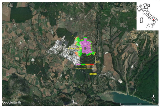
Figure 1.
Map of the study area: the VZI monitoring site, the COVA plant, the national road SS598, and the wind rose based on the hourly data at the VZI station over the study period (2013–2019).
2.2. Observational Dataset
Four gaseous pollutants—namely, nitrogen oxides (NOx), sulphur dioxide (SO2), carbon oxide (CO), and hydrogen sulphide (H2S), were selected for the analysis as proxies of anthropic sources existing in the area. For these pollutants, strong evidence of respiratory and cardiovascular health effects is documented [15,16]. Hourly data of NOx, SO2, CO, H2S, and of several meteorological variables (respectively, temperature (T), atmospheric pressure (P), relative humidity (RH), wind direction (wd), and wind speed (ws)), were downloaded from the official website of ARPAB [17] and combined to form the whole dataset used. Overall, a dataset consisting of more than 356,000 observations covering the 2013–2019 period was set up. The time series of all predictors considered respected the required 75% proportion of valid data. Subsequently, the data were daily averaged, and a set of other time-based variables was added to create the final dataset for the RF models development. In particular, the day of the week, the Julian day (number of days since 1 January, ‘Jday’), and the date Unix of the observations (number of seconds since 1 January 1970, ‘trend’) were included in the model development as proxies for local traffic sources and to account for seasonal and long-term variability, respectively.
2.3. Methodological Approach
The methodological approach to assess changes in pollutant concentrations levels, adopted in the present study, consists of the following main steps: (i) for each pollutant, an RF model was developed and, once its performances and interpretability had been analysed to ensure its reliability, the meteorological normalisation of the concentrations predicted by the RF model was carried out. (ii) After that, the estimation of the main change-points time location in the normalised signal and the trend analysis were performed. (iii) Combining the results of the previous stages with the available metadata, some hypotheses on the potential link between the normalised time series and specific events were formulated.
2.3.1. Meteorological Normalisation Procedure
The strategy for the meteorological normalisation follows the work described in [18], as subsequently implemented in [19,20], and was based on two steps: first, an RF model was built and validated for each of the pollutants analysed in the present study; second, the meteorological normalisation of the predicted pollutants concentrations was carried out.
In the development of each RF model (theoretical insight can be found [21]) the pollutant included in the dataset represented the dependent variable (or target), while meteorological and time-dependent features represented the explanatory variables (or predictors). In total, 80% of the whole observed dataset randomly sampled (training dataset) was used to build up the prediction model. The remaining 20% (testing dataset) was used to test the prediction accuracy of the model. The best model for each pollutant was built on the training dataset using the best combination of the tuning parameters selected on the basis of the R2 metric as evaluated on the testing dataset. The tuning parameters used in the work are the number of predictors randomly sampled to determine each split (mtry) and the minimum number of observations in a terminal node (min node size). The number of trees (n trees) was set at 1000. The RF model has an inherent procedure producing the relative importance of predictors, that is, the measure of the impact of each feature on the accuracy of the model. Thus, the relative importance resulting from the developed models was analysed to identify the most important predictors. The performances of the selected optimal RF model were fully assessed by comparing predicted and observed pollutants concentrations values using a set of statistical indicators [22] evaluated on the testing dataset (see Appendix A for the relevant equations).
Once established that the RF model explained an adequate amount of variance in the predicted air quality variable, it was used to predict the pollutant concentrations resampling only the meteorological explanatory variables from the whole study period without replacement and randomly allocating them to a dependent variable observation. The advantage of this procedure is that the normalisation process involves only the weather conditions but not the seasonal or weekly variations so that the resulting normalised series is more closely related to emissions changes rather than changes due to meteorological effects. This procedure was repeated a number of times (300), and then all the predictions were aggregated using the arithmetic mean to obtain the meteorological normalised concentration.
2.3.2. Trend and Structural Change Analysis
The goal of determining if there is a trend in the normalised concentrations over time was achieved using the Theil–Sen regression technique, which calculates the median slope of all possible slopes that may occur between the data points [23]. In our calculations, the trends were based on monthly averages, and they were adjusted for seasonal variations, as these can have a significant effect on monthly data. As far as the trend analysis is concerned, the unadjusted trends we estimated are the product of both emission and meteorological changes, while the weather-adjusted trends remove the influence of weather changes on air quality. Consequently, the difference between the unadjusted and weather-adjusted trends reflects the impact of meteorological changes or weather penalties.
For a more in-depth analysis of the trend thus achieved, an investigation about the structural changes in the normalised time series was carried out [24]. In the present study, we adopted the wild binary segmentation (wbs) change point detection method [25] to detect the number and potential locations of change points with no prior assumptions.
2.3.3. Metadata Analysis
Finally, an attempt was made to acquire the available appropriate metadata allowing to properly interpreting the results. Data concerning plant operation, the timing of significant events related to the plant activities, and the traffic flow patterns in the Agri Valley were examined. The former two were downloaded from official sources (i.e., the websites of the company that manages the plant) [26], while the traffic flow patterns of heavy and light vehicles concerning the national road SS 598 were provided by the Azienda Nazionale Autonoma delle Strade (ANAS) [27].
All data loading, processing, analysis, statistical modelling, and visualisation were performed in the R version 4.1.0 (R Foundation for Statistical Computing, Vienna, Austria). It was mainly used the Openair package for air quality and trend analysis [28], the rmweather package [11,18] for the meteorological normalisation, with the underlying ranger package [29], and tuneRanger package [30] for the development and tuning of the RF model, and the wbs package [31] for change points analysis.
3. Results and Discussion
3.1. Statistical Analysis
The descriptive statistics per year and pollutant are reported in Table 1.

Table 1.
Statistical summary of hourly data of NOx, SO2, CO, H2S registered at the VZI monitoring station from January 2013 to December 2019. Mean concentration and, in rounded brackets, the min and maximum values.
For regulated pollutants, time series analysis showed general compliance with the limits set for by the existing national [32] and European legislation [5]. It is worth noting that, for the sole Agri Valley, a regional law [33] identifies limit values more stringent than those in force at the national level for SO2 and H2S that are considered proxies of local hydrocarbon emissive processes. This law sets at 280 μg/m3 and 100 μg/m3 the hourly and daily limit values for the protection of human health for SO2, and 32 μg/m3 the daily limit for H2S. The hourly limit value for SO2 rarely exceeded these limits and each time in different years. As far as the climate is concerned, the cold and rainy winters as well as cool summers with frequent rainfall [34], typically registered in the area, define an area at sub-continental climate. Based on the analysis of wind data, the mean value of ws was 1.8 ms−1, with the higher values generally measured during daytime. The wind rose, superimposed on the map in Figure 1, showed a prevailing wind direction from the SW to NW sector, over the period ranging between January 2013 and December 2019.
3.2. RF Models Development and Performances
For each examined pollutant, the RF model, trained with the selection of the tuning parameters listed in Table 2, took the form shown by Equation (1) as follows:
where rf is the function implementing the random forest algorithm in the R software environment.
Table 2.
RF model tuning parameters for each of the selected pollutants.
The RF models’ performances were evaluated through the statistical indicators, whose resulting values were summarised in Table 3.
Table 3.
Statistical indicators of RF model performances for the testing dataset. Legend: R2 = coefficient of determination, MBE = mean bias error, MAE = mean absolute error, RMSE = root mean square error and IoA = index of agreement.
The R2 values show that the RF models can explain about 70% of the total NOx, CO, and H2S variability, while the model showed a moderate explanatory ability for SO2 (R2 values of 0.46).
The relative importance of the selected predictors for the examined pollutants is presented in Figure 2.
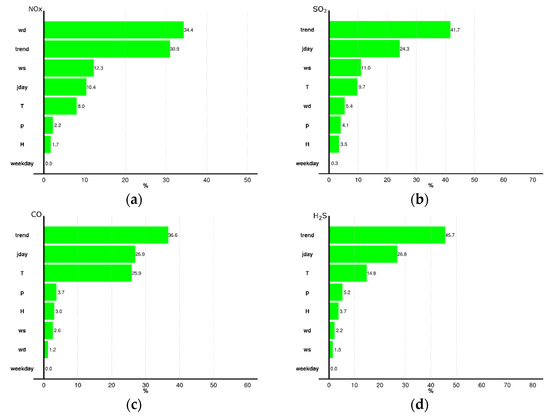
Figure 2.
Relative importance of predictors for the selected pollutants: (a) NOx, (b) SO2, (c) CO, and (d) H2S.
The overall contribution of the top four predictors explained over 85% of the variance for NO2 and SO2 and over 90% of the variance for CO and H2S. For SO2, CO, and H2S, the temporal variables, i.e., trend and Jday, were the most important predictors, indicating in the seasonality and long-term trend the strongest driving features.
The most important contributing factor to NOx variability, instead, was the wind direction, closely followed by trend, and to a lesser extent, ws and Jday. It is worth examining more closely the dependence of NOx from wd. The bivariate polar plot (Figure 3a) confirmed the strong directionality of NOx concentrations associated with winds from WSW, that is, in the direction of both several of the COVA plant conveyed emissive sources and the SS598 national road. The hypothesis of a traffic contribution to NOx was supported by the analysis of the daily and weekly NOx pattern (Figure 3b,c). The former tends to be significantly bimodal (higher concentrations in the early morning and late afternoon coinciding with the commuting hours). The latter shows a clear decrease in NOx concentrations on Saturday and Sunday when traffic is usually lower. Both these patterns were also confirmed by the analysis of the metadata concerning the traffic flows of cars and heavy vehicles for the national road SS598 provided by ANAS for the year 2019 (Figure 3d).
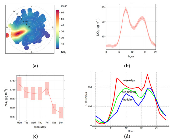
Figure 3.
Polar plot (a), daily (b) and weekly (c) profiles of hourly NOx concentrations. Additionally, shown in plots (b,c) is the 95% confidence interval in the mean. (d) The average hourly trend of traffic flows of the national road SS598 in 2019.
3.3. Meteorologically Normalised Air Pollutants Time Series
Daily concentrations of the observed and normalised data for NOx, SO2, CO, and H2S are shown in Figure 3. Additionally, shown in the figure is a blue solid line representing the line joining the wbs change points. As a result of the meteorological normalisation process, clear differences can be seen between the observed and normalised concentrations, with the latter being a much smoother data series. The trend in the normalised pollutants concentrations was less volatile and noisy, compared to the observed values and showed the extent to which changes in emissions influence the pollution level measured at the examined site. Moreover, the number and location of change points identified by the wbs methods appear to detect the main structural changes in the normalised time series. Linking these structural changes with specific events through the available metadata should allow formulating hypotheses about what originated them. It is worth dwelling on two specific events corresponding to the periods represented by the grey areas in Figure 4. By means of the available metadata at [26], it is known that the first corresponds to a plant shutdown, from April to August 2016, for judicial investigations.
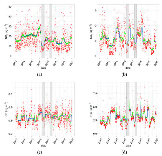
Figure 4.
Daily averages of observed (red dots) and meteorologically normalised concentrations (green lines) of (a) NOx, (b) SO2, (c) CO, and (d) H2S. The blue solid line represents the line joining the wbs change points, while the grey areas show the periods of COVA plant shutdowns.
The second consists of another plant shutdown, from April to July 2017, due to a major accident, caused by the release of hydrocarbons from a storage unit. As far as the SO2 and CO signals are concerned, a decrease in concentrations corresponding to these periods can be observed in Figure 4. With respect to the NOx pollutant, a strong correspondence was found between the normalised concentrations trend and the event that occurred at the COVA plant in 2016. The lack of correspondence with the event registered in 2017 may be due to other sources contributing to the observed NOx level. H2S, instead, seems to be less affected by these closures period, as expected, since this pollutant is representative of the fugitive emissions from oil tanks and piping of the COVA plant.
The results seem to confirm the goodness of this approach in identifying an atmospheric response in the observed data after an unplanned event or a change in emission sources. However, more stringent lines of evidence are desirable to confirm this hypothesis, due to the extreme complexity of the overall effects of the start/stop plant procedures on air quality.
Finally, Table 4 summarises the results of the Theil–Sen regression analysis. For NOx, a statistically significant trend for normalised and observed data was found, while less statistically significant normalised trends were found for H2S and CO (p < 0.05) and SO2 (p < 0.1).
Table 4.
Theil–Sen slope and 95% confidence intervals of the observed and normalised pollutants concentrations. The symbols shown next to the square bracket relate to how statistically significant the trend estimate is: p < 0.001 = ***, p < 0.01 = **, p < 0.05 = * and p < 0.1 = +.
The comparison between the observed and normalised slopes of each pollutant shows a generally scarce influence of the weather conditions on the trend of the pollutants. This result appears to be more stringent in the case of NOx due to the high statistical significance of the Theil–Sen analysis. This is consistent with the information deduced from the results illustrated above, which indicate in the local NOx sources, mainly the COVA plant and the traffic, the main drivers of NOx variability.
4. Conclusions
Ambient air pollution remains a great challenge for sustainable development and public health safeguard. Meteorological influences upon air quality trend analysis can complicate the evaluations of air pollution control efforts. The joined interpretation of the observed data of air pollutants, of the simulations produced by the RF models used to remove the effect of meteorology, and the subsequent statistical analysis adopted in the present study represents an effective tool to assess and quantify changes in air pollution. In particular, the technique of the meteorological normalisation allows discriminating the contribution of meteorology from those of source’s emissions, while the wbs method seems to be promising in correctly following main changes in the normalised pollutants concentrations. Since the RF models are data driven, caution is required when generalising the obtained results to different conditions and/or sites. Moreover, a deeper knowledge of the study area characterised by a complex orography, a more comprehensive collection of the available metadata, as well as a wider awareness of all natural or anthropic events affecting local air quality, can be obtained only through close collaboration with the local environmental and health authorities, who are the most informed on the criticalities of the examined territory.
Overall, our results show that the adopted procedure can improve qualitative trend assessment of observed air pollutants data and help in revealing shifts in pollutants levels that cannot be clearly seen in the original data, thus providing crucial information for the implementation of effective strategies to prevent the health impact of air pollution.
Author Contributions
All individuals listed as authors have equally contributed to the present work. All authors have read and agreed to the published version of the manuscript.
Funding
This research received no external funding.
Institutional Review Board Statement
Not applicable
Informed Consent Statement
Not applicable.
Data Availability Statement
Acknowledgments
The authors are grateful to the Environmental Protection Agency of Basilicata Region and ANAS for providing the data used in this work.
Conflicts of Interest
The authors declare no conflict of interest.
Appendix A
| Statistic Name | Equation |
| Mean Bias Error | |
| Mean Absolute Error | |
| Root Mean Squared Error | |
| Coefficient of Determination | |
| dex of Agreement | , when , when with c = 2 |
| where: = total number of hourly measurements; = ith predicted value; = ith observed value; = mean of the predicted values; = mean of the observed values | |
References
- Khomenko, S.; Cirach, M.; Pereira-Barboza, E.; Mueller, N.; Barrera-Gómez, J.; Rojas-Rueda, D.; de Hoogh, K.; Hoek, G.; Nieuwenhuijsen, M. Premature mortality due to air pollution in European cities: A health impact assessment. Lancet 2021, 5, e121–e134. [Google Scholar] [CrossRef]
- Available online: https://www.who.int/health-topics/air-pollution (accessed on 10 January 2021).
- World Health Organization. Air Quality Guidelines for Particulate Matter, Ozone, Nitrogen Dioxide and Sulfur Dioxide; World Health Organization: Geneva, Switzerland, 2005. [Google Scholar]
- Donateo, A.; Villani, M.; Lo Feudo, T.; Chianese, E. Recent Adavences of Air Pollution Studies in Italy. Atmosphere 2020, 11, 1054. [Google Scholar] [CrossRef]
- European Commission. Directive 2008/50/EC on Ambient Air Quality and Cleaner Air for Europe. Off. J. Eur. Union 2008, L152, 1–44. [Google Scholar]
- October Infringements Package: Key Decisions. Available online: https://ec.europa.eu/commission/presscorner/detail/IT/INF_20_1687 (accessed on 10 January 2021).
- Elminir, H.K. Dependence of urban air pollutants on meteorology. Sci. Total Environ. 2005, 350, 225–237. [Google Scholar] [CrossRef] [PubMed]
- Jones, A.M.; Harrison, R.M.; Baker, J. The wind speed dependence of the concentrations of airborne particulate and NOx. Atmos. Environ. 2010, 44, 1682–1690. [Google Scholar] [CrossRef]
- Kinney, P. Climate Change, Air Quality, and Human Health. Am. J. Prev. Med. 2008, 35, 459–467. [Google Scholar] [CrossRef]
- Petetin, H.; Bowdalo, D.; Soret, A.; Guervara, M.; Jorba, O.; Serradell, K.; Perez Garcia-Pardo, C. Meteorology-normalized impact of COVID-19 lokdown upon NO2 pollution in Spain. Atmos. Chem. Phys. 2020, 20, 11119–11141. [Google Scholar] [CrossRef]
- Grange, S.; Carslaw, D.; Lewis, A.; Boleti, E.; Hueglin, C. Random forest meteorological normalisation models for Swiss PM10 trend analysis. Atmos. Chem. Phys. 2018, 18, 6223–6239. [Google Scholar] [CrossRef] [Green Version]
- Guerreiro, C.B.B.; Foltescu, V.; de Leeuw, F. Air quality status and trends in Europe. Atmos. Environ. 2014, 98, 376–384. [Google Scholar] [CrossRef] [Green Version]
- Xiong, L.; Guo, S. Trend test and change-point detection for the Yichang hydrological station annual discharge series of the Yangtze River at the Yichang hydrological station/Test de tendance et détection de rupture appliqués aux séries de débit annuel du fleuve Yangtze à la station hydrologique de Yichang. Hydrol. Sci. J. 2004, 49, 99–112. [Google Scholar]
- Gagliardi, R.V.; Andenna, C. A Machine Learning Approach to Investigate the Surface Ozone Behaviour. Atmosphere 2020, 11, 1173. [Google Scholar] [CrossRef]
- Air Quality and Health. Available online: https://www.who.int/teams/environment-climate-change-and-health/air-quality-and-health/health-impacts (accessed on 10 January 2021).
- Mousa, H.A.L. Short-term effects of subchronic low-level hydrogen sulfide exposure on oil field workers. Environ. Health Prev. Med. 2015, 20, 12–17. [Google Scholar] [CrossRef] [Green Version]
- Gli Open Data-Qualità Dell’aria. Available online: www.arpab.it/opendata/q_aria_serie.asp (accessed on 10 January 2021).
- Grange, S.; Carslaw, D. Using meteorological normalisation to detect interventions in air quality time series. Sci. Total Environ. 2019, 653, 578–588. [Google Scholar] [CrossRef] [PubMed]
- Vu, T.V.; Shi, Z.; Cheng, J.; Zhang, Q.; He, K.; Wang, S. Harrison, R.M. Assessing the impact of clean air action on air quality trends in Beijing using a machine learning technique. Atmos. Chem. Phys. 2019, 19, 11303–11314. [Google Scholar] [CrossRef] [Green Version]
- Shi, Z.; Song, C.; Liu, B.; Lu, G.; Xu, J.; Vu, T.; Elliot, R.; Li, W.; Bloss, W.; Harrison, R. Abrupt but smaller than expected changes in surface air quality attributable to COVID-19 lockdowns. Sci. Adv. 2021, 7, 1–10. [Google Scholar] [CrossRef]
- Breiman, L. Random Forests. Mach. Learn. 2001, 45, 5–32. [Google Scholar] [CrossRef] [Green Version]
- Sayegh, A.S.; Munir, S.; Habeebullah, T.M. Comparing the Performance of Statistical Models for Predicting PM10. Aerosol Air Qual. Res. 2014, 14, 653–665. [Google Scholar] [CrossRef] [Green Version]
- Nunifu, T.; Fu, L. Methods and Procedures for Trend Analysis of Air Quality Data; Government of Alberta, Ministry of the Environment and Parks: Edmonton, ON, Canada, 2019.
- Aminikhanghahi, S.; Cook, D.J. A Survey of Methods for Time Series Change Point Detection. Knowl. Inf. Syst. 2017, 51, 339–367. [Google Scholar] [CrossRef] [Green Version]
- Fryzlewicz, P. Wild binary segmentation for multiple change-point detection. Ann. Stat. 2014, 42, 2243–2281. [Google Scholar] [CrossRef]
- ENI in Basilicata. Available online: https://www.eni.com/eni-basilicata/news/2021-elenco-news.page (accessed on 1 February 2021).
- ANAS-Le Strade. Available online: https://www.stradeanas.it/it/strade (accessed on 30 March 2021).
- Carslaw, D. Openair-An R package for air quality data analysis. Environ. Model. Softw. 2012, 27, 52–61. [Google Scholar] [CrossRef]
- Wright, M.; Ziegler, A. ranger: A fast implementation of random forests for high dimensional data in <C++ and R. J. Stat. Softw. 2017, 77, 1–17. [Google Scholar]
- Probst, P.; Wright, M.; Boulestei, A. Hyperparameters and Tuning Strategies for Random Forest. 2019. Available online: https://arxiv.org/pdf/1804.03515.pdf (accessed on 30 March 2021).
- Baranowski, R.; Fryzlewicz, P. Wild Binary Segmentation for Multiple Change-Point Detection. R WBS Package Documentation Version 1.4. 2019. Available online: https://cran.r-project.org/web/packages/wbs/wbs.pdf (accessed on 30 March 2021).
- Legislative Decree 155/10. Attuazione della Direttiva 2008/50/CE relativa alla qualità dell’aria ambiente e per un’aria più pulita in Europa. Gazz. Uff. 2010, 216, 1–111. [Google Scholar]
- Norme tecniche ed azioni per la tutela della qualità dell’aria nei comuni di Viggiano e Grumento Nova. In Proceedings of the Delibera Giunta Regionale della Regione Basilicata, Basilicata, Italy, 6 August 2013. n. 983.
- PEE Centro Olio Val d’Agri di Viggiano—Edizione 2013. Available online: http://www.prefettura.it/potenza/contenuti/Pee_centro_olio_val_d_agri_di_viggiano_edizione_2013-64403.htm (accessed on 30 March 2021).
Publisher’s Note: MDPI stays neutral with regard to jurisdictional claims in published maps and institutional affiliations. |
© 2021 by the authors. Licensee MDPI, Basel, Switzerland. This article is an open access article distributed under the terms and conditions of the Creative Commons Attribution (CC BY) license (https://creativecommons.org/licenses/by/4.0/).