Surrogate Modeling of MODTRAN Physical Radiative Transfer Code Using Deep-Learning Regression ^†

Abstract

Radiative Transfer Models (RTMs) are one of the major building blocks of remote-sensing data analysis that are widely used for various tasks such as atmospheric correction of satellite imagery. Although high-fidelity physical RTMs such as MODTRAN are considered to offer the best possible modeling of atmospheric procedures, they are computationally demanding and require a lot of parameters that should be tuned by an expert. Therefore, there is a need for surrogate models for the physical RTM codes that can mitigate these drawbacks while offering an acceptable performance. This study aimed to suggest surrogate models for the MODTRAN RTM using deep-learning models. For this purpose, the top of atmosphere (TOA) spectra calculated by the MODTRAN code as well as the bottom of atmosphere (BOA) input spectra and other atmospheric parameters such as temperature and water vapor content observations were collected and used as the training dataset. Two deep-learning regression models, including a fully connected network (FCN) and an auto-encoder (AE), as well as a random forest (RF) machine-learning regression model were trained. The results of these models were assessed using the three evaluation metrics root mean squared error (RMSE), regression coefficient (R²), and spectral angle mapper (SAM). The evaluations indicated that the AE offered the best performance in all the metrics, with RMSE, R², and SAM scores of 0.0087, 0.9906, and 1.4295 degrees, respectively, in the best-case scenarios. These results showed that deep-learning models can better reproduce results via high-fidelity physical RTMs.

1. Introduction

Radiative transfer models (RTMs) are not only fundamental in the radiometric calibration of satellite sensors, but they are also extensively used for the atmospheric correction of satellite data. These models solve the differential equation but are computationally demanding [1]. There is a need for surrogate models based on deep learning that can mitigate this issue while offering accurate outputs.

Deep learning is widely used in a wide variety of remote-sensing applications, such as change detection [2] and binary segmentation [3]. There have been multiple cases of emulating RTMs using deep learning. Pal et al. [4] suggested a surrogate model for the shortwave and longwave radiative transfer model SP-E3SM based on deep neural networks (DNNs). Their model achieved 8–10 times faster run times while having an accuracy of 90–95%. Lagerquist et al. [5] emulated the shortwave Rapid Radiative Transfer Model (RRTM) with a UNet++ model. Their models proved to be about 10⁴ times faster than the original model. Aiming to find a faster way of running the Bayesian Atmospheric Radiative Transfer (BART) code, Himes et al. [6] used a neural network approach. The results demonstrated that the emulator was about 80–180 times faster than BART when run on GPU. Yao et al. [7] compared different deep-learning models. Bidirectional Recurrent Neural Networks (BRNNs) were found to offer the best performance.

Although there are other similar studies [8], this research is the first to leverage the extensive dataset from the RadCalNet portal [9] to develop an emulator for the MODTRAN RTM. Fully connected and autoencoder deep-learning models are developed using this dataset and compared to the random forest machine-learning model.

2. Dataset

In 2014, the Infrared Visible Optical Sensors (IVOS) and the Committee on Earth Observation Satellites (CEOS) Working Group on Calibration and Validation (WGCV) introduced the international calibration network RadCalNet [9]. This network comprises four international calibration test sites that offer top-of-atmosphere (TOA) reflectance data in the nadir view, collected at 30 m intervals between 9 a.m. and 3 p.m. local standard time. This data is available at 10 nm intervals, ranging from 400 nm to 2500 nm of the electromagnetic spectrum. These measurements are derived from ground-level nadir-view reflectance readings, coupled with six atmospheric parameters including surface pressure, temperature, columnar water vapor, columnar ozone, aerosol optical depth, and the angstrom coefficient. To standardize the data processing, a correction to TOA values is applied uniformly across all sites using the Modtran RTM.

The GONA and RVUS sites in RadCalNet have the highest number of measurements; thus, only these two pseudo-invariant sites have been used in this study. The GONA calibration site is located in Gobabeb, Namibia and is characterized by a sandy desert terrain, covering a circular region with a 30 m radius. There have been 13,385 measurement pairs of surface reflectance spectrum and atmospheric parameters on this site since 2015. The spectral range is from 400 nm to 2300 nm with a gap between 1820 nm and 1910 nm bands.

The RVUS site is located in Railroad Valley, a desert region in the state of Nevada, USA, which is surrounded by mountains to the east and west. This area is generally flat with less than 3 m of elevation variation and spans 1 km by 1 km. So far, 17,348 measurements of BOA spectrum and atmospheric parameters have been collected on this site. The spectral range is from 400 nm to 2300 nm with a gap between 1810 nm and 1960 nm bands.

Some of the observations in the datasets were noisy and needed to be filtered out as outliers. This was achieved by excluding every data sample outside the confidence level of three times the standard deviation. Six other parameters have been concatenated with the six atmospheric parameters to make a complementary feature set of 12 elements. These six parameters include the measurement time and date, aerosol type, azimuth and zenith angles of the sun, and earth to sun distance. A major part of the preprocessing was to rescale the 12 complementary parameters in the range of 0 and 1 to facilitate the training of models. The final step was to randomly select 70 percent of the data samples for training and the remaining for testing.

3. Methodology

The main goal of this study is to develop a surrogate multivariate regression model that can take the measured BOA spectra along with the complementary parameters as inputs and estimate the TOA spectra. Atmospheric radiative processes that MODTRAN calculates have a completely non-linear nature, and more sophisticated machine-learning models are required to reproduce MODTRAN outputs. That is the reason why only random forest was employed as a machine-learning model in this study, which is widely considered one of the best regression models. Thus, fully connected network (FCN) and convolutional autoencoder (AE) deep-learning models along with a random forest model have been trained separately on the datasets gathered from the two calibration sites.

3.1. Fully Connected Network (FCN)

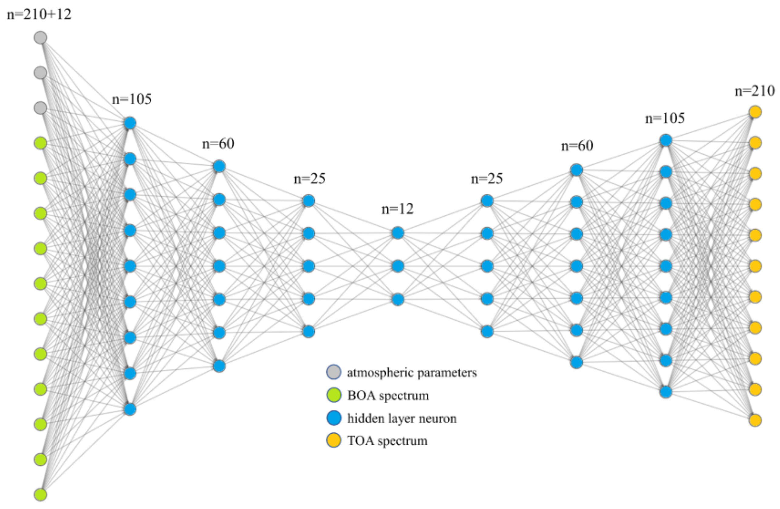
The fully connected model presented in this study is designed to take an input vector of 222 dimensions. This vector is the concatenation of the BOA spectrum (210 variables) with the corresponding complementary parameters (12 variables). The outputs of the model have a dimension of 210, equal to the number of TOA spectral bands. As can be seen in Figure 1, the model architecture follows an encoder-decoder structure, suitable for problems with matching input and output dimensions. The number of layers and neurons in this model are adjusted in a way that closely resembles the architecture of the other deep-learning model, allowing for a fair comparison of the performance of these two architectures.

The ReLU has been chosen as the activation function for the hidden layers and is widely used in deep networks. Additionally, since the problem is of a regression type, the activation function for the last layer has been chosen to be Linear. To train the model, the Adam optimizer with a learning rate of 0.0003 has been used. Finally, the model is compiled with the mean square error (MSE) loss function, suitable for regression problems.

3.2. Autoencoder

An autoencoder (AE) is designed to extract representative features from input vectors based on two fundamental components: the encoder and the decoder. The key point in these networks is that the input layer dimension should match the output layer dimension. Initially, the encoder part performs feature extraction on input data and reduces their dimensions. Then, the decoder part maps the features back to the output. 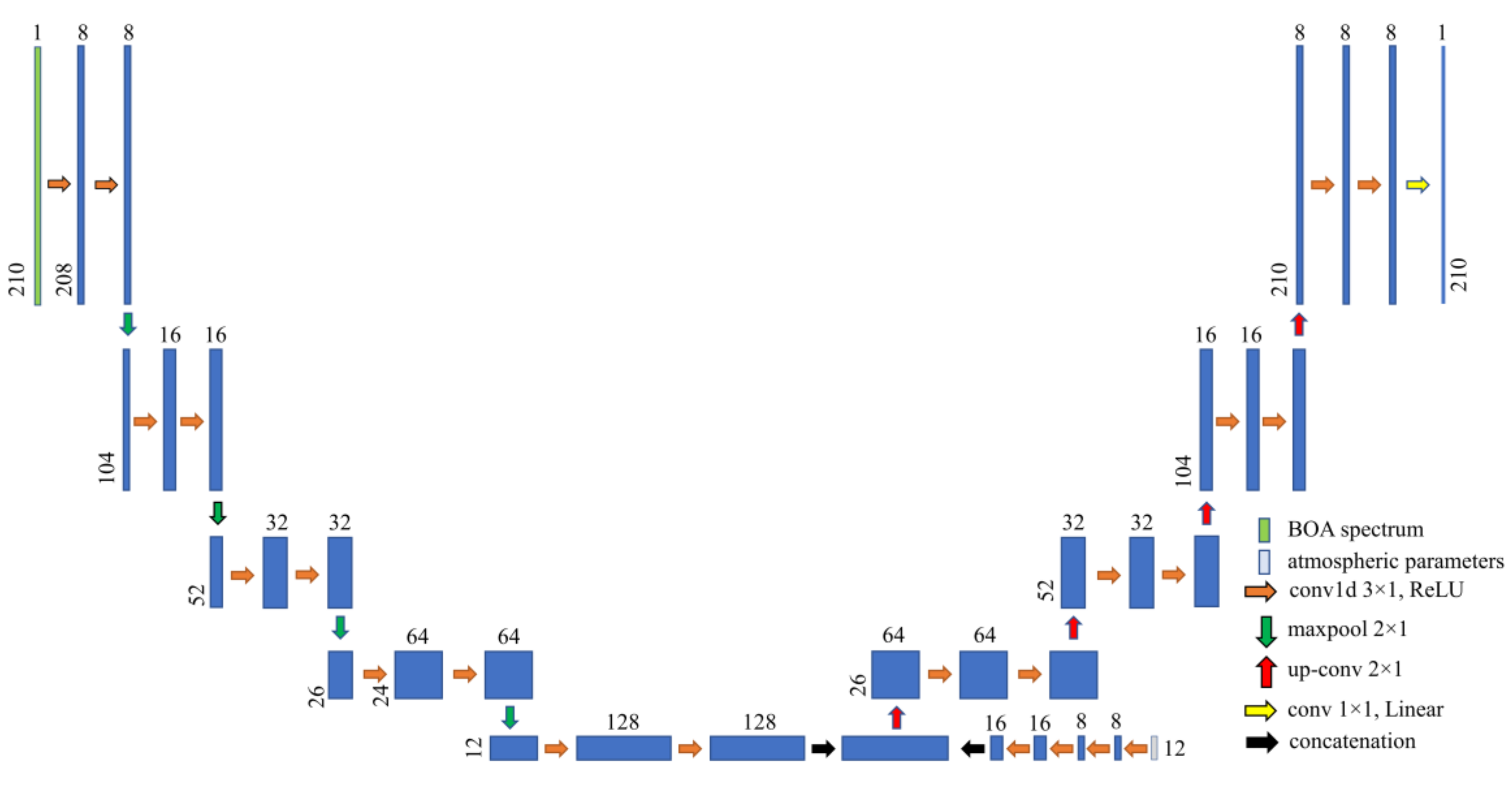Figure 2 illustrates the architecture of the autoencoder network developed in this study.

The maxpooling operator just takes the largest value in its search window and omits other information. Therefore, to prevent the loss of some of the complementary parameters, the concatenation approach has not been used in this model. Instead, the 12 complementary parameters have been fed to the model in the bottleneck section after the encoding of BOA spectra. The activation functions, loss function, and optimizer are the same as in the previous model, but in this model, a learning rate of 0.0001 has been adopted.

4. Results and Discussion

To assess the accuracy of trained models, root mean square error (RMSE) and coefficient of determination (R²) metrics have been utilized. Since the regression problem in this study produces output vectors, the spectral angle mapper (SAM) metric can indicate the deviation of the predictions of surrogate models from the MODTRAN outputs in degree units. The formula for the SAM metric is as follows, where $Y$ and $\widehat{Y}$ represent the actual and predicted spectra, respectively.

$$SAM=\arccos \left(\frac{Y.\widehat{Y}}{\left|Y\right|\left|\widehat{Y}\right|}\right)$$

(1)

4.1. GONA Site Results

The quantitative results of the surrogate modeling for the GONA site are reported in

Table 1. Quantitative results of the surrogate modeling for the GONA and RVUS sites.

	GONA			RVUS
Models	R2	RMSE	SAM (Degree)	R2	RMSE	SAM (Degree)
RF	0.9507	0.0207	2.7302	0.9469	0.0212	2.6254
FC	0.9332	0.0243	4.1760	0.9719	0.0150	2.6605
AE	0.9823	0.0116	1.9832	0.9906	0.0087	1.4295

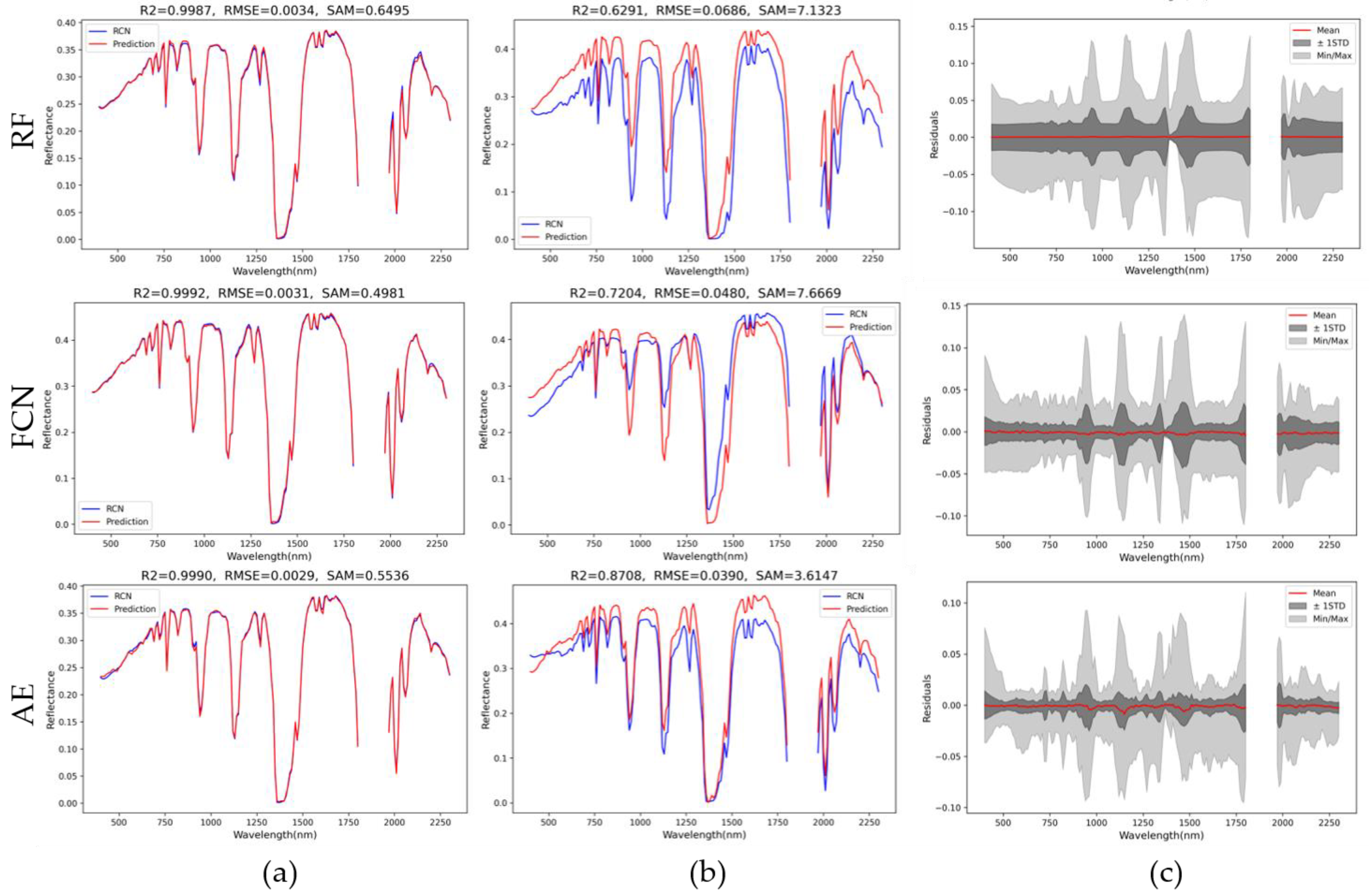
, presenting the values of evaluation metrics for 4011 testing spectra. Moreover, Figure 3 illustrates the visual results. The autoencoder had the best performance in all the metrics in the GONA dataset, with R2, RMSE, and SAM scores of 0.9823, 0.0116, and 1.9832 degrees, respectively.

The second highest scores belonged to the random forest model, while the fully connected model achieved the worst outputs with an RMSE of 0.0243. It should be noted that the RMSEs in this study are in the unit of surface reflectance. The visual results illustrated in Figure 3 reflect the same quantitative results. The residuals’ range was the narrowest in the autoencoder, and random forest had smoother means compared to the fully connected model.

4.2. RVUS Site Results

The quantitative results of the surrogate modeling for the RVUS site are reported in Table 1, presenting the values of evaluation metrics for 5205 testing spectra. Moreover, Figure 4 illustrates the visual results. Also, in the RVUS dataset, the autoencoder achieved the best results with R2, RMSE, and SAM scores of 0.9906, 0.0097, and 1.4295 degrees.

The fully connected model was better than random forest in terms of R2 and RMSE scores (0.9716 and 0.0150, respectively); however, random forest had a slightly higher SAM score (2.6254 degrees), indicating its better ability to model the shape of the spectrum. The overall smoothest residuals’ mean belonged to the random forest model, although the error range was the largest. The autoencoder had the narrowest residuals’ range, but the means were slightly noisy.

5. Conclusions

Developing surrogate models for computationally demanding physical radiative transfer models is of great importance in reducing computation costs. This study aimed to accomplish this task by using deep-learning models to find a link between the inputs and outputs of MODTRAN RTM. For this purpose, training datasets were gathered from the GONA and RVUS calibration sites of the RadCalNet portal. Fully connected and autoencoder deep-learning models were employed to solve the regression problem. Moreover, a random forest model was used for comparison. The results indicated that the autoencoder model had the best performance in both datasets, with RMSE, R², and SAM scores of 0.0087, 0.9906, and 1.4295 degrees, respectively, in the best-case scenarios. Furthermore, random forest outperformed the fully connected model in the GONA dataset in all the evaluation metrics, while the fully connected model had better RMSE and R² scores in the RVUS dataset. Although other studies have found a regression method to be appropriate [8], the main contribution of this research is the utilization of the RadCalNet dataset.

References

- Liang, X.; Liu, Q. Applying Deep Learning to Clear-Sky Radiance Simulation for VIIRS with Community Radiative Transfer Model—Part 1: Develop AI-Based Clear-Sky Mask. Remote Sens. 2021, 13, 222. [Google Scholar] [CrossRef]
- Aghdami-Nia, M.; Shah-Hosseini, R.; Salmani, M. Effect of transferring pre-trained weights on a Siamese change detection network. ISPRS Ann. Photogramm. Remote Sens. Spat. Inf. Sci. 2023, 10, 19–24. [Google Scholar] [CrossRef]
- Abbasi, M.; Shah-Hosseini, R.; Aghdami-Nia, M. Sentinel-1 Polarization Comparison for Flood Segmentation Using Deep Learning. Proceedings 2023, 87, 14. [Google Scholar] [CrossRef]
- Pal, A.; Mahajan, S.; Norman, M.R. Using Deep Neural Networks as Cost-Effective Surrogate Models for Super-Parameterized E3SM Radiative Transfer. Geophys. Res. Lett. 2019, 46, 6069–6079. [Google Scholar] [CrossRef]
- Lagerquist, R.; Turner, D.; Ebert-Uphoff, I.; Stewart, J.; Hagerty, V. Using Deep Learning to Emulate and Accelerate a Radiative Transfer Model. J. Atmos. Ocean. Technol. 2021, 38, 1673–1696. [Google Scholar] [CrossRef]
- Himes, M.D.; Harrington, J.; Cobb, A.D.; Baydin, A.G.; Soboczenski, F.; O’Beirne, M.D.; Zorzan, S.; Wright, D.C.; Scheffer, Z.; Domagal-Goldman, S.D.; et al. Accurate Machine-Learning Atmospheric Retrieval via a Neural-Network Surrogate Model for Radiative Transfer. Planet. Sci. J. 2022, 3, 91. [Google Scholar] [CrossRef]
- Yao, Y.; Zhong, X.; Zheng, Y.; Wang, Z. A Physics-Incorporated Deep Learning Framework for Parameterization of Atmospheric Radiative Transfer. J. Adv. Model. Earth Syst. 2023, 15, e2022MS003445. [Google Scholar] [CrossRef]
- Servera, J.V.; Rivera-Caicedo, J.P.; Verrelst, J.; Munoz-Mari, J.; Sabater, N.; Berthelot, B.; Camps-Valls, G.; Moreno, J. Systematic Assessment of MODTRAN Emulators for Atmospheric Correction. IEEE Trans. Geosci. Remote Sens. 2022, 60. [Google Scholar] [CrossRef]
- Bouvet, M.; Thome, K.; Berthelot, B.; Bialek, A.; Czapla-Myers, J.; Fox, N.P.; Goryl, P.; Henry, P.; Ma, L.; Marcq, S.; et al. RadCalNet: A Radiometric Calibration Network for Earth Observing Imagers Operating in the Visible to Shortwave Infrared Spectral Range. Remote Sens. 2019, 11, 2401. [Google Scholar] [CrossRef]