Next Article in Journal
Towards More Efficient Hydraulic Modeling of Water Distribution Networks Using the EPANET Software Engine
Previous Article in Journal
Utilization of a Telemetry Monitoring System for the Dynamics of Water Quantity and Quality in the Dadahup Swamp Irrigation Area
 
 
Please note that, as of 4 December 2024, Environmental Sciences Proceedings has been renamed to Environmental and Earth Sciences Proceedings and is now published here.
Proceeding Paper

Comparison of the Performance of CMIP5 and CMIP6 in the Prediction of Rainfall Trends, Case Study Quebec City †

by
Amirhossein Salimi
1,
Tadros Ghobrial
1 and
Hossein Bonakdari
2,*
1
Department of Civil and Water Engineering, Université Laval, Quebec City, QC G1V0A6, Canada
2
Department of Civil Engineering, University of Ottawa, Ottawa, ON K1N6N5, Canada
*
Author to whom correspondence should be addressed.
Presented at the 7th International Electronic Conference on Water Sciences, 15–30 March 2023; Available online: https://ecws-7.sciforum.net.
Environ. Sci. Proc. 2023, 25(1), 42; https://doi.org/10.3390/ECWS-7-14243
Published: 16 March 2023
(This article belongs to the Proceedings of The 7th International Electronic Conference on Water Sciences)

Abstract

:
Climate change affects many meteorological parameters that could result in spatiotemporal variations of the hydrological cycle. These variations can affect local rainfall intensities or design storms; therefore, it is necessary to assess the local effects of climate change in different areas. Therefore, the current research aims at evaluating the accuracy of the precipitation data of the most recent Coupled Model Intercomparison Project phases 5 and 6 (CanESM2 from CMIP5 and CanESM5 from CMIP6 models), over a historical period from 1953 to 2010, as well as the predicted data for the future between 2010 and 2050 for the Quebec City rain gauge Station (Jean Lesage Intl). In this regard, precipitation data were analyzed using a statistical index to find the most accurate model for the study area. The results of this evaluation showed that CanESM5 is more accurate than CanESM2 for most of the evaluation indices. However, both of these models did not perform well since the precipitation prediction for CanESM5 (as the accurate model) R index was 0.48 for the monthly and was 0.75 in the seasonal scale. In addition, the Bias index revealed that both models underestimated rainfall prediction with negative index values for both scales and models. The trend of future precipitation under socio–economic scenarios (4.5 (pessimistic) and 8.5 (optimistic)) shows that the changes in future precipitation are not significant. In addition, for scenario 4.5, the trend of precipitation decreases for almost half of the year, while for scenario 8.5, the magnitude of the decrease and the number of months with a decreasing trend of precipitation are significantly reduced when compared to scenario 4.5.

1. Introduction

Global warming has caused significant changes in the climate. In recent years, the severity of droughts, floods and extreme events has increased in different parts of the globe. The Intergovernmental Panel on Climate Change (IPCC) was established to identify its effects and especially how human activities affect it. In order to conduct climate change studies, climate variables under the influence of greenhouse gas emissions must first be simulated [1].
One of the important consequences of climate change is the change in the meteorological parameters’ trend, especially the precipitation trend [2]. Therefore, a great deal of research has been conducted to evaluate climate change’s effect on extreme rainfall events. These studies showed that global warming is affecting and causing climate changes based on the Coupled Model Intercomparison Project Phase 5 (CMIP5) and Coupled Model Intercomparison Project Phase 6 (CMIP6) climate reports in Canada [3]. Compared to other methods such as the multi-model ensemble (MME), the CMIP5 and CMIP6 models showed better performance. In addition, various methods can be used to reduce their uncertainty [4]. With the release of the sixth report (CMIP6), the desire to examine the performance of this report compared to the fifth report (CMIP5) has increased among researchers. One of the major improvements in CMIP6 is the introduction of socio–economic scenarios [5]. Examining the difference between the data from the report 5 and 6 climate models for temperature and precipitation shows that for the fixed time intervals, most of the temperature indices show higher predicted changes in CMIP6 when compared to CMIP5 in Canada. Rainfall changes in CMIP6 mainly occurred in extreme precipitation indices [3]. However, it is clear that the method of General Circulation Models (GCM) ensembles can lead to different estimates of future mean changes and different levels of uncertainty in those estimates [4]. Overall, current research has shown that the CMIP6 ensemble provides a narrower band of the uncertainty of future climate projections specifically for North America and brings more confidence to hydrological impact studies [6]. The importance of such analysis is in assessing risk and future vulnerability, and implementing efficient measures to control the changes made in the flow of rivers and their ability to warn of floods [5,7].
It is necessary to examine the system’s response as a general unit for determining the possible effects of climate changes such as the increase in the concentration of greenhouse gases and the impact of socio–economic activities on the climate system [5]. For this purpose, it seems necessary to use climate models. These models include the main stages that occur in the climate system and calculate the corrections of different components when responding to the changes in the forcing factors. Therefore, evaluating the accuracy of the data of these models and choosing the most efficient and adaptable models are important and necessary steps for any forecasting [8]. This assessment is more important for precipitation, which has a more significant behavioral complexity than other meteorological phenomena. Therefore, identifying the mechanism and evaluating the effectiveness of atmospheric general circulation models in estimating precipitation and knowing their temporal and spatial frequency significantly affects the preparedness for such extreme events. Therefore, in this research, the effectiveness of the CMIP5 and CMIP6 for predicting extreme rainfall events is assessed, and the future trend of rainfall reported by the superior model is evaluated.

2. Methods and Materials

2.1. Data and Models

Monthly precipitation records of the Jean Lesage Intl Station (Figure 1) were collected from Canada Gov. historical meteorology data records [9]. The data-set period was from 1953 to 2020 (67 years). In addition, the CMIP5 and CMIP6 models were used to investigate the accuracy and evaluate future climate change under different scenarios. For these purposes, 2 different models (one from each CMIP) were selected according to previous research results [3,5]. These models are reported in Table 1. The historical period for evaluating the accuracy of the selected models was chosen. For CMIP5, this period was between 1953 to 2005 and for CMIP6, the period from 1953 to 2010 was selected.

2.2. General Circulation Models

Climatic variables are simulated under the influence of increasing or decreasing greenhouse gases. There are different methods for this task; however, the most reliable is the use of atmospheric general circulation models or GCMs. GCMs can be used to understand the dynamics of the physical components of the atmosphere that are related to climate change phenomena. The purpose of using GCMs is to obtain spatial–temporal patterns of climate changes as well as long-term forecasting of climate variables [5]. Climate modeling is an important tool for understanding past, present and future climate changes [2]. In other words, currently the most reliable tool for investigating the effects of climate change on different systems is the use of a GCM. These models are able to model the trends of atmospheric and oceanic parameters for a long-term period using approved IPCC scenarios [2]. Their main weakness is the low spatial resolution and the simplification they consider for climate processes. To overcome the weakness of low resolution, it is necessary to scale the output of these models before using them in climate-change impact-assessment studies [1].

2.3. Mann–Kendall Trend Analysis

The Mann–Kendall method was first presented by Mann (1945) and then expanded and developed by Kendall (1970). Among the non-parametric tests, the Mann–Kendall test is the best choice for checking the uniform trend in series [10]. This test is used to determine the randomness and trend in the series. First, to determine the non-parametric nature of the statistical series, data are arranged and ranked in ascending order and then based on that, the randomness of the data with no trend is specified. If there is a trend in the data, then it is non-random.
The null hypothesis of the Mann–Kendall test indicates randomness and the absence of a trend in the data series, and the acceptance of the one hypothesis (rejection of the null hypothesis) indicates the existence of a trend in the data series [10].

2.4. Evaluation of Performance

Five types of statistical indices were employed to assess the performance of the CMIP data sets. The correlation coefficient (R) (Equation (1)) as a correlation-based index, Normalized Root Mean Square Error (NRMSE) (Equation (4)), Bias (Equation (2)), Root Mean Square Relative Error (RMSRE) (Equation (5)) and Slope (Equation (3)). The mathematical definitions of the mentioned indices are as follows:
R = i = 1 n y i y ¯ x i x ¯ i = 1 n y i y ¯ 2 i = 1 n x i x ¯ 2
B i a s = i = 1 n x i y i n
S L O P E = x i x ¯ y i y ¯ n 1 S 2 x
N R M S E = 1 y ¯ 1 n i = 1 n x i y i 2
R M S R E = 1 n i = 1 n x i y i y i 2
where xi and yi are the ith samples of the estimated and actual values (respectively), x ¯ and y ¯ are the average of the estimated and actual values (respectively), n is the number of samples, and S2x is the Variance of x.

3. Results

3.1. Evaluation the Performance of the Models

The performance of the CMIPs’ models is shown in Table 2, which reported the accuracy of the models to compare to the observation data. Five different indices were used for evaluation at two different time scales. Based on the correlation coefficient (R), CanESM5 had better performance when compared to the CanESM2 model. Nevertheless, the correlation coefficient on a monthly scale was poor since R values were less than 0.5, although if the scale changed to the seasonal, they improved ideally (between 0.65 and 0.75).
In addition, Normalized Root Mean Square Error (NRMSE) results showed that CanESM5 had better performance when compared to CanESM2 on the seasonal scale. These results are promising and show that the model can estimate precipitation within acceptable errors because the NRMSE values are close to one, which means that the deviations in precipitation estimates are small.
The RMSRE is a criterion similar to RMSE; their main difference is that RMSRE is divided by projected values. The best value for these criteria is 0, meaning there is no difference between projected and observed values. Based on Table 2, the CanESM5 model performed better with an RMSRE of 0.3 and 0.67 for the monthly and seasonal scales, respectively.
Mean Bias deviation shows the systematic error in the amount of precipitation. A value of zero indicates that the difference between the observed and predicted precipitation amount is not systematic, while a large Bias indicates that the amount of precipitation deviates greatly from the observed amount of precipitation. The fact that the Bias parameter is close to zero also indicates the model’s accuracy in the simulation. A negative Bias indicates underestimation, while a positive Bias indicates overestimation. Based on the results in Table 2, both models underestimated precipitation at this Station.
Finally, the Slope is used to assess the direction of the projection line or the angle coefficient. If the Slope is negative, the relationship between the two variables (X and Y) will be inverse, and the Slope expresses the amount of change in Y relative to each unit of change in X. For this index, a Slope of 1, or regression 1:1 between the two variables, means perfect correlation. The value of the Slope in Table 2 shows that the estimated data were far from the regression line (1:1) and the value of the Slope statistic for both models was equal to or less than 0.5.
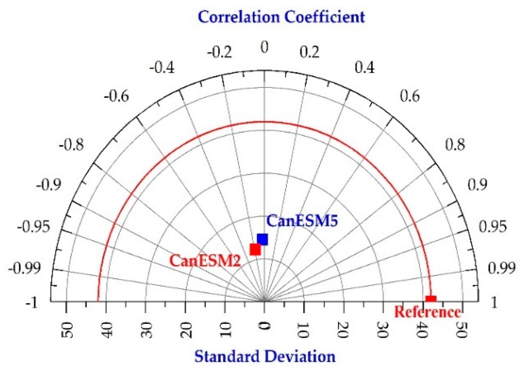
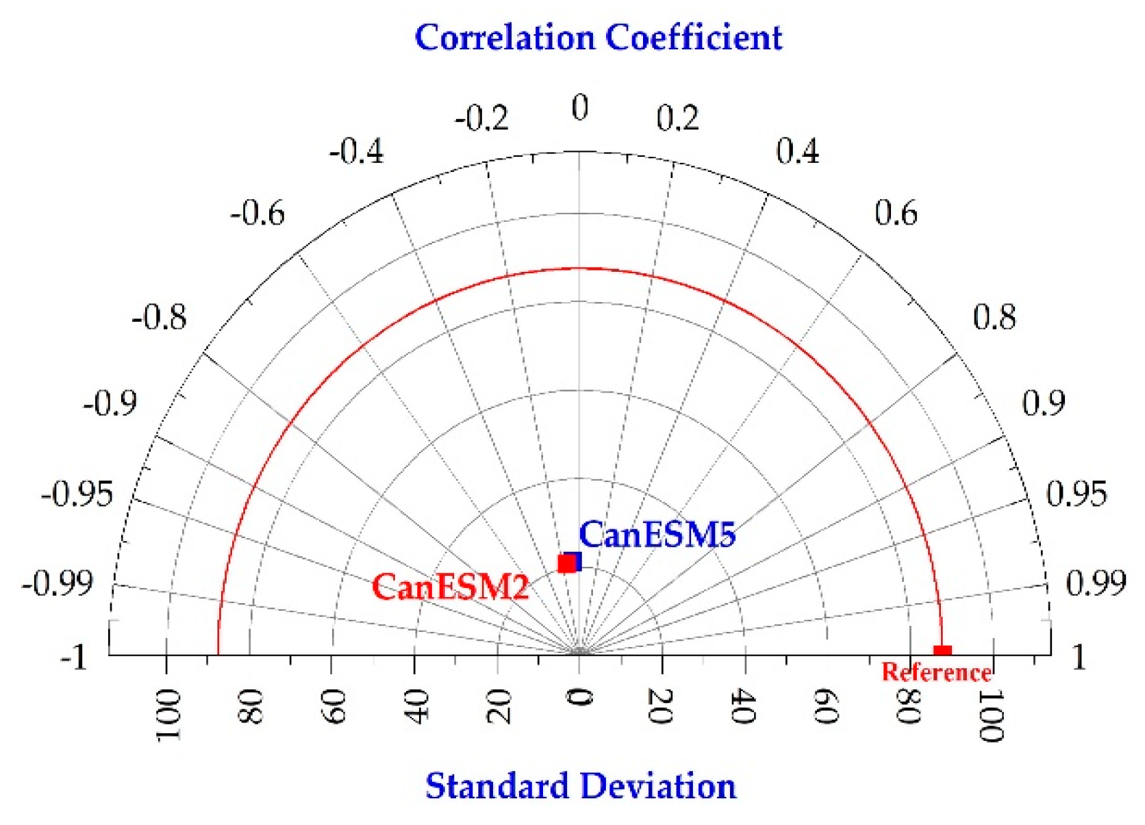
Taylor diagrams provide a visual framework for comparing a suite of variables from one or more test data sets to one or more reference data sets. Commonly, the test data sets are model experiments while the reference data set is a control experiment or some reference observations (e.g., Station data sets). Generally, the plotted values are derived from climatological monthly, seasonal or annual means. Because the different variables (e.g., precipitation, temperature) may have widely varying numerical values, the results are normalized by the reference variables. The normalized variances ratio indicates the model’s relative amplitude and observed variations [11]. Figure 2 and Figure 3 provide information about monthly and seasonal Taylor diagrams of the CanESM2 and CanESM5. It is clear that CanESM5′s performance on the monthly scale is better than CanESM2’s, although both models have poor performance on the seasonal scale. All in all, CanESM5 can provide better results compared to CanESM2.
In summary, the values obtained by the models show that the efficiency of the CanESM5 model in estimating the amount of precipitation was better than the CanESM2 model. In addition, due to the closeness of the indicators that take into account the number of deviations and compare the estimated and actual time series, the mentioned model can detect fluctuations and precipitation trends in the selected Station.

3.2. Precipitation Future Trend

It is more suitable to use non-parametric methods for series that cannot be fitted with a special statistical distribution and have high skewness or elongation. The Mann–Kendall test is one of the most common and widely used non-parametric trend analysis methods of time series. Data changes are identified using the Mann–Kendall method, and their type and time are determined [12]. According to the essential role of precipitation in providing water resources, it is vital to study the process of its changes in the future. This study will help the authorities with planning and managing water resources. Since international reports have delivered serious warnings about the crisis and even the physical lack of water in the future for different parts of the world, knowing the predicted variability of this important meteorological parameter is essential [13]. Although the evaluation of the models’ performance on historical data has shown that the models do not have a high ability to estimate the amount of precipitation, the comparison of the projected and observed time series shows a slight deviation and an acceptable agreement between the two data sets. Therefore, the future forecast of the precipitation by the selected model (CanESM5) is an effective step in understanding the precipitation pattern in the future.
Table 3 presents the Mann–Kendall parameters (Test Z) for the different time-scale rainfall future trends (from 2020 to 2049) using the best-fit model (CanESM5) for the two socio–economic (SSP) scenarios. The selected SSP scenarios for this study were 4.5 (Pessimistic) and 8.5 (Optimistic). The time scales were Monthly (Jan to Dec), Seasonal (Spring to Winter) and Annual for the selected model’s scenarios (4.5 and 8.5). For scenario 4.5, rainfall changes were decreasing for February and June to August, while for other months, these changes were increasing. These outputs can be found based on Test Z values in Table 3. Moreover, rainfall changes in the seasonal scale were also decreasing in the Summer and Fall. Trend analysis results for May, for July in the monthly scale and for Summer and Fall in the seasonal scale showed that the downward trend was more intense since the value of Test Z (Kendall’s score) reached more than −1 in this period of time.
On the other hand, for scenario 8.5 (Table 3), rainfall changes were increasing in most of the months, although, like scenario 4.5, the decreasing trend remained. However, the intensity of the downward trend became less prominent when compared to scenario 4.5. In addition, rainfall changes in the spring tended to decrease, unlike the 4.5 scenario.

4. Conclusions

The results showed that the studied models do not have a high ability to estimate precipitation in the Jean Lesage Intl Station. According to the results of the studied statistics such as the correlation coefficient (R) and Slope, the accuracy of the models was poor and the correlation coefficient in all models was less than 0.5 on a monthly scale. However, in the seasonal scale, the correlation value was reached at 0.75 in the best model. The Slope index was also consistent with the correlation coefficient because in the two investigated models, the distribution of precipitation data was rarely very close to the regression line (1:1) and the Slope value was usually less than 0.5. In addition, the results of the two selected models were close to each other, but the CanESM5 model was more accurate than the other model in the studied Station. The deviation of the projected data and the Station data was very small, which can be shown based on the NRMSE index in all the investigated models as less than 2. In addition, in the selected Station, the Bias index indicated both models would underestimate the rainfall trend in both time scales. The comparison of the obtained findings showed that the present research results were largely consistent with some other researchers. For example, Hidalgo and Alfaro (2014) showed that most of the CMIP5 models have a low ability to estimate precipitation in the central regions of the United States [11]. Rupp et al. (2013) showed that although the CMIP5 model rainfall data have less accuracy compared to other grided data such as NCEP and ERA40, they estimate the seasonal cycle of precipitation with the same accuracy as networked data in the northwestern regions of America [12]. Mehran et al. (2014) concluded that the CMIP5 model rainfall data are consistent with GPCP data in most parts of the world but do not perform well in dry areas [13]. Ebtehaj and Bonakdari (2023) concluded that the results of the comparison of the CanESM5 and CanESM2 models strongly depend on the month and season, and that the results of CanESM5 are slightly better compared to the other model [5].
Finally, the precipitation trend analysis results for the CanESM5 model and under the two scenarios 4.5 and 8.5 showed that the trend of precipitation changes at the Jean Lesage Intl Station will not be significant. In addition, in scenario 4.5, the precipitation trend decreased in almost half of the year, while in scenario 8.5, the intensity of the decrease and the number of months with a decreasing trend of precipitation were significantly reduced.

Author Contributions

Conceptualization, H.B. and T.G.; methodology, H.B.; software, A.S.; validation, A.S. and H.B.; formal analysis, A.S.; investigation, A.S.; resources, H.B.; data curation, H.B.; writing—original draft preparation, A.S.; writing—review and editing, T.G. and H.B.; visualization, A.S.; supervision, T.G. and H.B.; project administration, T.G.; funding acquisition, H.B. All authors have read and agreed to the published version of the manuscript.

Funding

This project is partially funded by the ESSOR–MARTHE-ET-ROBERT-MÉNARD scholarship administered by CentrEau (Centre québécois de recherche sur la gestion de l’eau) and the Government of Québec Ministère de Sécurité Publique (MSP) under the project ‘Compréhension du comportement des rivières en hiver et mesures de gestion des risques liés aux inondations (FLUTEIS; CPS-18-19-26)’.

Institutional Review Board Statement

Not applicable.

Informed Consent Statement

Not applicable.

Data Availability Statement

GCM datasets are available at Copernicus Climate Change Service, Climate Data Store, (2021): CMIP6 climate projections. Copernicus Climate Change Service (C3S) Climate Data Store (CDS). DOI:10.24381/cds.c866074c (accessed on 25 November 2022).

Conflicts of Interest

The authors declare no conflict of interest.

References

  1. Salimi, A.H.; Masoompour Samakosh, J.; Sharifi, E.; Hassanvand, M.R.; Noori, A.; von Rautenkranz, H. Optimized artificial neural networks-based methods for statistical downscaling of gridded precipitation data. Water 2019, 11, 1653. [Google Scholar] [CrossRef]
  2. IPCC. Summary for Policy Markers Climate Change: The Physical Science Basis. In Contribution of Working Group I to the Fourth Assessment Report of the Intergovernmental Panel on Climate Change; Cambridge University Press: Cambridge, UK, 2007; p. 881. [Google Scholar]
  3. Sobie, S.R.; Zwiers, F.W.; Curry, C.L. Climate Model Projections for Canada: A Comparison of CMIP5 and CMIP6. Atmos. Ocean. 2021, 59, 269–284. [Google Scholar] [CrossRef]
  4. Lovejoy, S. The Future of Climate Modelling: Weather Details, Macro weather Stochastics—Or both? Meteorology 2022, 1, 414–449. [Google Scholar] [CrossRef]
  5. Ebtehaj, I.; Bonakdari, H. A comprehensive comparison of the fifth and sixth phases of the coupled model intercomparison project based on the Canadian earth system models in spatio-temporal variability of long-term flood susceptibility using remote sensing and flood frequency analysis. J. Hydrol. 2023, 617, 128851. [Google Scholar]
  6. Martel, J.L.; Brissette, F.; Troin, M.; Arsenault, R.; Chen, J.; Su, T.; Lucas-Picher, P. CMIP5 and CMIP6 model projection comparison for hydrological impacts over North America. Geophys. Res. Lett. 2022, 49, e2022GL098364. [Google Scholar] [CrossRef]
  7. Miara, A.; Macknick, J.E.; Vörösmarty, C.J.; Tidwell, V.C.; Newmark, R.; Fekete, B. Climate and water resource change impacts and adaptation potential for US power supply. Nat. Clim. Chang. 2017, 7, 793–798. [Google Scholar] [CrossRef]
  8. Eyring, V.; Gleckler, P.J.; Heinze, C.; Stouffer, R.J.; Taylor, K.E.; Balaji, V.; Guilyardi, E.; Joussaume, S.; Kindermann, S.; Lawrence, B.N.; et al. Towards improved and more routine Earth system model evaluation in CMIP. Earth Syst. Dyn. 2016, 7, 813–830. [Google Scholar]
  9. Extracted from the Environment and Climate Change Canada Historical Climate Data. Available online: https://climate.weather.gc.ca/index_e.html (accessed on 4 December 2022).
  10. Hussain, M.; Mahmud, I. pyMannKendall: A python package for non-parametric Mann Kendall family of trend tests. J. Open Source Softw. 2019, 4, 1556. [Google Scholar] [CrossRef]
  11. Hidalgo, H.G.; Alfaro, E.J. Skill of CMIP5 Climate Models in Reproducing 20th Century Basic Climate Features in Central America. Int. J. Climatol. 2014, 35, 3397–3421. [Google Scholar] [CrossRef]
  12. Rupp, D.E.; Abatzoglou, J.T.; Hegewisch, K.; Mote, M. Evaluation of CMIP5 20th century climate simulations for the Pacific Northwest USA. J. Geophys. Res. Atmos. 2013, 118, 10884–10906. [Google Scholar] [CrossRef]
  13. Mehran, A.; AghaKouchak, A.; Phillips, T.J. Evaluation of CMIP5 continental precipitation simulations relative to satellite-based gauge-adjusted observations. J. Geophys. Res. 2014, 119, 1695–1707. [Google Scholar] [CrossRef]
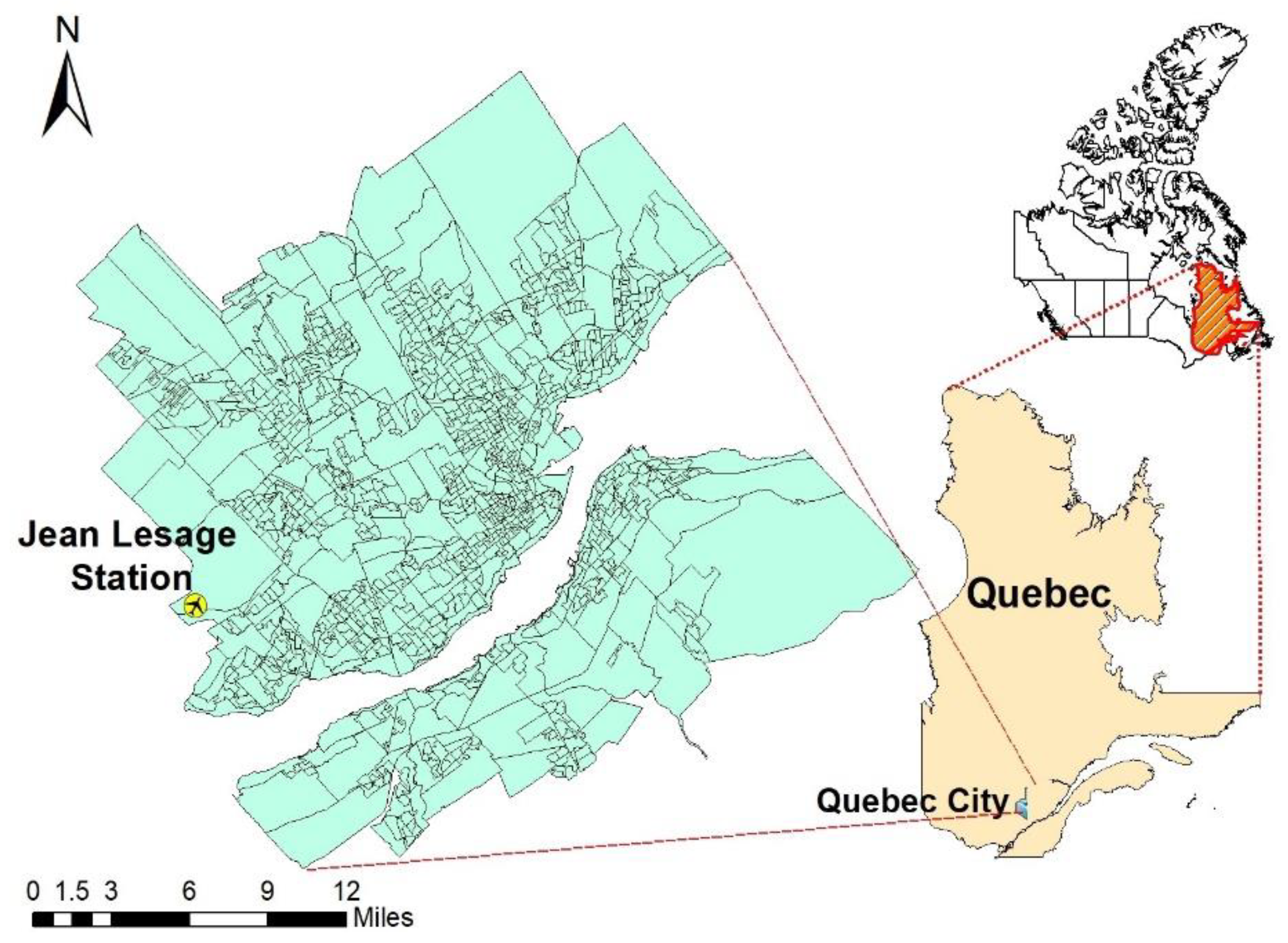
Figure 1. Selected Station position.
Environsciproc 25 00042 g001
Figure 2. Models’ performance in monthly scale.
Environsciproc 25 00042 g002
Figure 3. Models’ performance in seasonal scale.
Environsciproc 25 00042 g003
Table 1. The selected CMIP models.
ModelCMIPScenarioResolution
CanESM25RCP
2.6, 4.5, 8.5
0.5 × 0.5
CanESM56SSP
2.6, 4.5, 8.5
0.5 × 0.5
Table 2. Performance of CMIP models.
ModelScaleRNRMSERMSREBiasSlope
CanESM2Monthly0.430.400.36−85.6−0.30
CanESM50.480.540.30−58.70.20
CanESM2Seasonal0.651.510.96−11.80.50
CanESM50.751.080.67−10.30.13
Table 3. Mann–Kendall test Z values for 4.5 and 8.5 scenarios.
Time Series4.5 Test Z8.5 Test ZTime Series4.5 Test Z8.5 Test Z
Jan.1.480.04Jul.−1.781.89
Feb.−0.300.25Aug.−0.361.53
Mar.0.16−0.71Sep.1.300.14
Apr.−0.43−0.79Oct.2.022.86
May.−1.071.46Nov.1.300.18
Jun.−0.46−0.09Dec.1.481.71
Spring0.71−0.18
Summer−1.250.39Annual0.002.82
Fall−1.322.32
Winter1.782.21
Disclaimer/Publisher’s Note: The statements, opinions and data contained in all publications are solely those of the individual author(s) and contributor(s) and not of MDPI and/or the editor(s). MDPI and/or the editor(s) disclaim responsibility for any injury to people or property resulting from any ideas, methods, instructions or products referred to in the content.