Estimating the Potential Evapotranspiration of Egypt Using a Regional Climate Model and a High-Resolution Reanalysis Dataset ^†

Abstract

Station observation is a good data source to monitor the potential evapotranspiration (PET) changes of a specific site particularly for the purpose of crop irrigation activities; however it represents only the site geographic characteristics and provides real-time/historical records. Hence, there was an urgent need to find a promising tool and a simple empirical to predict/project the PET in locations where station observation is not feasible. The Hargreaves–Samani method (HS) is recommended after the Penman−Monteith equation. To address this issue, the Regional Climate Modeling version 4 (RegCM4) with spatial resolution 25 km was used to compute the PET using the HS for the period 1979–2017. Era-Interim reanalysis of 1.5 degrees (EIN15) and NCEP/NCAR reanalysis version 2 of 2.5 degrees (NNRP2) were used to examine the influence of the lateral boundary condition on the simulated PET. The two simulations were designated as EIN15-RegCM4 and NNRP2-RegCM4, respectively. To examine the possible influences on the simulated PET, a comparison was conducted between EIN15-RegCM4 and NNRP2-RegCM4. After that, a comparison was conducted between the original HS formula (HS) and its calibrated version (HSnew) with respect to the 0.1−degree ERA5-land derived reanalysis product (hereafter ERA5) using EIN15-RegCM4 (as an example). Results showed that switching between EIN15 and NNRP2 did not show a notable influence on the simulated PET. Further, calibrating the HS coefficients indicates a considerable improvement in estimating the PET (relative to the original equation) when it is compared with ERA5. Such improvement is confirmed by a significant low mean bias. Over the majority of locations, the RegCM4 shows a good performance using the calibrated HS equation. In conclusion, the RegCM4 can be used to estimate the PET using the calibrated HS either for making a daily forecast or for projecting the future PET under different global warming scenarios.

1. Introduction

Potential evapotranspiration (PET) plays an important role in the global terrestrial hydrology cycle. Additionally, PET is used for calculating the water needs of different crops and assessing hydrological and meteorological droughts, water balance analysis, and designing and operating irrigation projects [1]. The authors of [2] reported that, the Penman−Monteith (PM) equation is the standard model to compute the PET on various time scales. However, the authors of [3] reported that computing PET (using PM) is not recommended for arid/hyper-arid regions because it requires a surplus of soil moisture and it requires a large number of meteorological variables, which leads to greater uncertainty of the estimated PET.

PET can be computed using simple empirical models, such as temperature-based methods [4,5], radiation-based methods [6] and physically processed-based models (e.g., [2]). Additionally, the authors of [2] reported that the Hargreaves−Samani (HS) method can be recommended directly after PM and it can operate on daily/monthly time scales. Estimating the PET (using HS equation) showed a reliable performance in computing the PET with respect to observations as reported by [7,8]. Further, calibrating the HS showed a reliable performance in computing the PET with respect to PM observations [9,10,11]. Recently, the authors of [3] calibrated the regional climate model (RegCM4) output using the Climate Research Unit (CRU) and a linear regression model (LRM) at specific locations. However, calibrating the coefficients of the HS equation over Egypt and the role of the lateral boundary condition (used to downscale the RegCM4) in simulating the PET were not considered until the present day. Therefore, the present study aims to:

• Examine the influence of the lateral boundary condition (EIN15 and NNRP2) on the simulated PET with respect to ERA5−land−derived product (hereafter ERA5; [12]).
• Address the added value of the calibrated HS equation (relative to the original version) in comparison with the ERA5.
• Validate the calibrated HS equation (versus the original version) by examining the climatological annual cycle of the simulated PET with respect to ERA5 at locations defined by [3].

Section 2 describes the study area and experiment design; Section 3 shows the results of the study. Section 4 provides the discussion and conclusion.

2. Materials and Methods

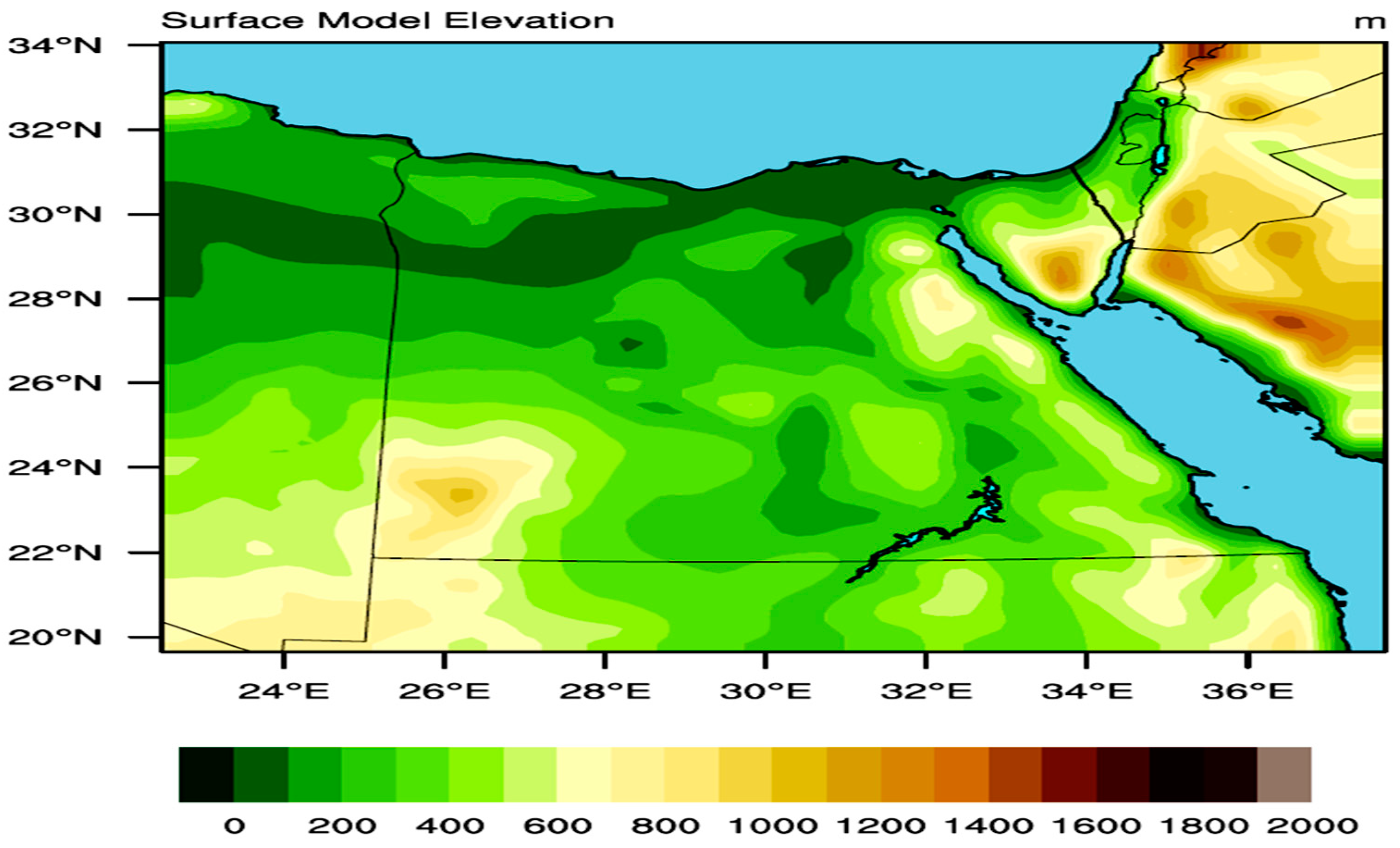
2.1. Study Area

A brief description of the study area is available in [3]; model domain dimension is covered in Section 2.2.

2.2. Model Description and Experiment Design

This study used the Abdus Salam International Centre for Theoretical Physics (ICTP) regional climate model version 4.7 (hereafter RegCM-4.7.0; [13]). The RegCM is a broad model used for conducting long-term simulations and future regional climate projections in Intercomparison projects [14]. To address the influence of the lateral boundary condition on the simulated PET, two experiments were conducted over the period 1979–2017. The first two years were considered as spin-up to properly initialize the RegCM4 model following [15], so the actual analysis starts at 1981 and ends at 2017. The two experiments adopted both ERA-Interim reanalysis of 1.5 degrees (EIN15; [16]) and NCEP/NCAR reanalysis version 2 of 2.5 degrees (NNRP2; [17]) to downscale the RegCM4 model. The RegCM4 model domain (Figure 1) was customized with grid spacing of 25 km with 60 grid points in both zonal and meridional directions centered at 27° latitude and 30° longitude. Additionally, the following physical schemes were used in the present study: Emanuel convection scheme over land and ocean [18], radiation scheme of [19] and Holtslag boundary layer scheme [20]. The simulated PET was calculated using the default HS equation as:

$${\mathrm{P}\mathrm{E}\mathrm{T}}_{\mathrm{H}\mathrm{S}}=0.0135\times \mathrm{S}\mathrm{W}\times (\mathrm{T}2\mathrm{m}+17.8)$$

(1)

The calibrated version is written as

$${\mathrm{P}\mathrm{E}\mathrm{T}}_{\mathrm{H}\mathrm{S}}=0.0105\times \mathrm{S}\mathrm{W}\times (\mathrm{T}2\mathrm{m}+17.8)$$

(2)

Several attempts have been made to obtain a reasonable bias of the calibrated HS equation (using ERA5 as the observational dataset). It was found that swtiching the radiation coefficient from 0.0135 to 0.0105 gave more promising results than calibrating the temperature coefficient (17.8). Note that SW (global incident solar radiation) is expressed in units of mm day⁻¹ to show how much energy is used to evaporate water [2] and T2m is the 2-m mean air temperature (in °C).

2.3. Validation Data

Various reanalysis products were used to evaluate the RegCM4 performance:

• ERA5 ([21]): It provides hourly estimates of a large number of atmospheric, land, and oceanic climate variables with 0.25° horizontal grid spacing and 137 vertical levels (up to a height of 80 km). For the purpose of the present study, monthly means were aggregated to the seasonal time scale.
• ERA5land ([22]): This product provides the surface meteorological variables at high resolution (0.1 degrees) using the land surface model of the ERA5 (titled ECMWF Scheme for Surface Exchanges over Land incorporating land surface hydrology; H-TESSEL).

• Please note that both ERA5 and ERA5land were used to evaluate the simulated SW and T2m of the RegCM4 (since these fields were used as inputs of the HS equation) to take into account the influence of the horizontal grid spacing of the reanalysis product.

3.

Station observation is a major source to monitor the PET changes both spatially and temporally. However, availability of long-term records was not sufficient to evaluate the RegCM4 performance (before and after calibrating the HS equation) in this study. Recently, a new high-resolution global gridded PET (hPET) product was developed [12]. This product uses the hourly meteorological variables provided by the offline land model of the ERA5 reanalysis product [21]. Additionally, it adopts the PM equation to compute the PET and it is integrated over the period 1981–2021 in 0.1-degree grid spacing over the global land area. In the present study, monthly mean PET data were used to evaluate the RegCM4 performance both spatially and for locations defined by [3] in Section 1.

For the purpose of the present study, all products were bilinearly interpolated on the RegCM4 curvilinear grid following [10,15].

3. Results

Before assessing the performance of the RegCM4 (in simulating the PET), it is important to quantify the RegCM4 model bias concerning the simulated SW and T2m (as inputs of the HS equation). Figure S1 shows the simulated SW with respect to ERA5 and ERA5land as well as the difference between ERA5 and ERA5land themselves for the seasons: March−April−May (MAM), June−July−August (JJA), September−October−November (SON) and December−January−February (DJF). From Figure S1, it can be noticed that the RegCM4 is able to reproduce the spatial pattern of the SW with respect to ERA5 and ERA5land in all seasons (Figure S1a–c,g–i,m–o,s–u). Additionally, the RegCM4 overestimates the SW in the MAM season by 10–30 W m⁻² (Figure S1d,e). In the JJA and SON, the RegCM4 bias ranges from 20 to 40 W m⁻² (Figure S1j,k,p,q). Lastly in the DJF, the RegCM4 bias becomes 10–20 W m⁻² with respect to both products (Figure S1v,w). Further, there is no noted difference between ERA5 and ERA5land in all seasons (Figure S1f,l,r,x). It can be noted that the RegCM4 bias is maximized in the JJA and SON and it is minimized in the DJF.

Like SW, the RegCM4 shows a good ability to capture the spatial pattern of the simulated T2m with respect to reanalysis products in all seasons (Figure S2a–c,g—i,m–o,s–u). Additionally, there is no observable difference between ERA5 and ERA5land (Figure S2f,l,r,x), which means that the resolution of the observational dataset does not affect the evaluation of the RegCM4. In addition, an obvious warm-bias is noted in all seasons ranging from 3 to 7 °C (Figure S2d,e,j,k,p,q,v,w) with mostly pronounced warm bias during the summer. Such noted bias can be attributed to the fact that land cover of Egypt is mostly represented by desert leading to a low specific/relative humidity. As a result, the convective activity is affected, producing low total cloud cover (not shown), high SW approaching the earth surface and eventually warming the earth surface and the adjacent air layer close to the earth surface. Another possible reason is that the Holtslag scheme is characterized by high turbulent activity, leading to an enhancement of the warming effect produced by the SW.

3.1. Influence of Lateral Boundary Condition

To examine the influence of the lateral boundary condition on the simulated PET, Equation 1 was used to compute the simulated PET. Figure 2 shows the simulated PET (by the EIN15-RegCM4 and NNRP2-RegCM4, respectively) with respect to the ERA5. From Figure 2, it can be noted that the RegCM4 shows good consistency in reproducing the spatial pattern of the simulated PET in comparison with the ERA5 product (see Figure 2a−c,g−i,m−o,s−u). Additionally, it can be observed that there is no significant difference between EIN15 and NNRP2 in all seasons (Figure 2f,l,r,x). Such behavior can be attributed to two reasons: 1—RegCM4 has a similar performance when it is driven either by EIN15 or NNRP2 [23] and 2—RegCM4’s physical parameterization dominates over the lateral boundary condition [24]. In addition, it can be observed that both simulations have a bias of 1–2.5 mm day⁻¹ in the March−April−May season (MAM; Figure 2d,e).

The bias approaches its maximum in the June−July−August season because the RegCM4 shows a bias of 1–4.5 mm day⁻¹ overall Egypt (JJA; Figure 2j,k). In the September-October-November (SON) season, the bias ranges between 1 and 3 mm day⁻¹ over coastal regions and middle Egypt and 1–1.5 mm day⁻¹ over Upper Egypt (see Figure 2p,q). Lastly, in the December-January-February (DJF) season, the bias is around 0.5–2 mm day⁻¹ over majority of Egypt (Figure 2v,w). From a simple check between Figures S1 and S2 and Figure 2; it can be noted that the PET spatial pattern is more consistent with the SW than T2m. Therefore, calibrating the SW coefficient is more effective than T2m (see Equation (2)). This point will be discussed briefly in Section 3.2.

3.2. Added Value of the Calibrated HS Equation

As noted in Section 3.1, there is no significant difference between the two simulations. Therefore, the RegCM4-EIN15 simulation was taken (as an example) to examine the added value of the calibrated HS equation compared to ERA5. Figure 3 shows the simulated PET before calibration (HS), after calibration (HSnew) in comparison with the ERA5 and the difference between HSnew and HS. In general, both simulations are able to capture the spatial pattern of the simulated PET against the ERA5 (Figure 3a–c,g–i,m–o,s–u). However, HSnew shows added value over the HS in all seasons particularly in the JJA. Such value is indicated in two points: 1—better ability to reproduce the PET spatial pattern relative to HS and 2—the RegCM4 bias is significantly reduced in all seasons (particularly in the JJA) compared to the HS. For instance, in the MAM season, the HS shows a bias of 1–2.5 mm day⁻¹ over the entire domain (Figure 3d). On the other hand, the HSnew shows a bias of 0.5 mm day⁻¹ over the majority of Egypt, with some regions approaching 0.5–1 mm day⁻¹ and 0.5 to −1.5 mm day⁻¹ around Lake Nasser (Figure 3e). Qualitatively, the HSnew reduces the PET by 0.6–1.2 mm day⁻¹ relative to the HS (Figure 3f).

In the JJA and SON seasons, the HS overestimates the PET over all of Egypt by 1–4.5 mm day⁻¹ (see Figure 3j,p). After calibration, the HSnew reduces the PET bias to 0.5–1.5 mm day⁻¹ over the north coast of Egypt and the western desert and −0.5 mm day⁻¹ around Lake Nasser and middle Egypt (see Figure 3k,q). From a qualitative point of view, the HSnew approximately reduces the simulated PET by 1.6–2.2 mm day⁻¹ in the JJA (Figure 3l) and by 0.8–1.6 mm day⁻¹ in the SON (Figure 3r). Lastly, in the DJF, it can be observed that HSnew shows its added value over the HS in middle and upper Egypt where the bias was 0.5–2 mm day⁻¹ prior to calibration (Figure 3v) and became 0.5–1 mm day⁻¹ post calibration (Figure 3w). Further, the HSnew approximately reduces the PET by 0.4–1.2 mm day⁻¹ relative to the HS (see Figure 3x). Overall, it can be noted that the added value of the HSnew (over the HS) can be arranged according to season in the following order: 1—JJA; 2—SON; 3—MAM; and 4—DJF. These findings are in agreement with the results reported in Figure S1.

To further explore the added value of the calibrated HS, the climatological annual cycle (Figure 4) of the simulated PET of the HS and HSnew (compared to ERA5) was plotted for locations reported by [3]. Only Port-Said was not mentioned because it shows missing values. From Figure 4, it can be observed that the performance of HS/HSnew varies with location and month. For instance, the HS is close to ERA5 in the months of January, February, November and December, while HSnew is close to ERA5 for the rest of the months in Alexandria. For Arish, Marsa-Matruh and Ismailia; HSnew is closer to ERA5 than HS. In Giza and Asswan, the situation is quite different because HS performs better than HSnew in all months. Further, HSnew shows an improved performance over HS in Assyut. Additionally, the situation in Luxor is similar to the one observed in Alexandria. Finally, in Siwa, Dakhla and Kharga, HSnew shows an improved performance (relative to the HS) in comparison with the ERA5.

4. Discussion and Conclusions

Potential evapotranspiration (PET) is important for monitoring hydrological and meteorological droughts as well as assessing the crop irrigation needs. Additionally, it is a major component in the global terrestrial hydrology cycle. Therefore, the availability of long-term records of PET on a hierarchy of time scales (ranging from hourly to seasonal) is important. The authors of [2] recommend the PM model to compute the PET because it is based on the physical exchange of water and energy between vegetation and atmosphere; however, it requires a large number of meteorological variables (which may not be available for a long time for a variety of locations). Further, uncertainty of the involved meteorological variables may induce a source of uncertainty in the computed PET (and in particular if they are derived from reanalysis products/regional climate models). In addition, it requires a surplus of soil moisture (which is not suitable for the domain of the present study). Hence, there was an urgent need to compute the PET with a simple empirical method (only needs a few meteorological inputs).

Among various empirical methods, the HS model was chosen in this study because it gives a good performance with observational datasets of the PM [7,8,9,10,11]. However, the HS has not been calibrated in Egypt until today. In the present study, the regional climate model (RegCM4) was used to compute the PET comparing between the non-calibrated/calibrated HS with respect to ERA5. The influence of the lateral boundary condition on the simulated PET was also examined. The results showed that switching between EIN15 and NNRP2 did not show a considerable impact on the simulated PET (Figure 2). Spatially, the calibrated HS showed its added value (relative to the original HS model) particularly in the JJA season; such value can be seen by a reduction in the PET bias with respect to the ERA5 (Figure 3). On a point scale, the HS/HSnew performance varies with location and month (Figure 4). Nevertheless, the calibrated HS model can be recommended to construct a regional map of PET of Egypt, predict the daily PET for locations (where station observations are not available) and project the future PET under different global warming scenarios [10,15]. To ensure more robust results of the simulated PET (using the calibrated HS model), a future work will consider the following points:

• Revising the short/longwave radiation scheme, tuning the parameters of the boundary layer scheme to possibly reduce the uncertainty of the simulated SW, T2m and, eventually PET.
• Adapting a bias-correction technique (e.g., [3]) to correct the simulated PET over a location of interest.
• Studying the influence of climate change on the PET of Egypt using the calibrated HS equation [25] and CMIP5/6 simulations [10,15,26].

References

1. Abdullah, S.S.; Malek, M.A.; Abdullah, N.S.; Kisi, O.; Yap, K.S. Extreme learning machines: A new approach for prediction of reference evapotranspiration. J. Hydrol. 2015, 527, 184–195. [Google Scholar] [CrossRef]
2. Allen, G.R.; Pereira, S.L.; Raes, D.; Smith, M. Crop Evapotranspiration: Guidelines for Computing Crop Water Requirements; Report 56; Food and Agricultural Organization of the United Nations (FAO): Rome, Italy, 1998; 300p. [Google Scholar]
3. Anwar, S.A.; Salah, Z.; Khaled, W.; Zakey, A.S. Projecting the Potential Evapotranspiration in Egypt Using a High-Resolution Regional Climate Model (RegCM4). Environ. Sci. Proc. 2022, 19, 43. [Google Scholar] [CrossRef]
4. Hargreaves, G.L.; Samani, Z.A. Reference crop evapotranspiration from temperature. Appl. Eng. Agric. 1985, 1, 96–99. [Google Scholar] [CrossRef]
5. Hargreaves, G.L.; Allen, R.G. History and evaluation of Hargreaves evapotranspiration equation. J. Irrigat. Drain. Eng. 2003, 129, 53–63. [Google Scholar] [CrossRef]
6. Irmak, S.; Irmak, A.; Allen, R.G.; Jones, J.W. Solar and Net Radiation-Based Equations to Estimate Reference Evapotranspiration in Humid Climates. J. Irrig. Drain. Eng. 2003, 129, 5. [Google Scholar] [CrossRef]
7. Er-Raki, S.; Chehbouni, A.; Khabba, S.; Simonneaux, V.; Jarlan, L.; Ouldbba, A.; Rodriguez, J.C.; Allen, R. Assessment of reference evapotranspiration methods in semi-arid regions: Can weather forecast data be used as alternate of ground meteorological parameters? J. Arid. Environ. 2010, 74, 1587–1596. [Google Scholar] [CrossRef] [Green Version]
8. Potop, V.; Boroneant, C. Assessment of Potential Evapotranspiration at Chisinau Station; Mendel a Bioklimatologie: Brno, Czech Republic, 2014; pp. 3–5. [Google Scholar]
9. Sperna Weiland, F.C.; Tisseuil, C.; Dürr, H.H.; Vrac, M.; Van Beek, L.P.H. Selecting the optimal method to calculate daily global reference potential evaporation from CFSR reanalysis data for application in a hydrological model study. Hydrol. Earth Syst. Sci. 2012, 16, 983–1000. [Google Scholar] [CrossRef] [Green Version]
10. Anwar, S.A.; Mamadou, O.; Diallo, I.; Sylla, M.B. On the influence of vegetation cover changes and vegetation-runoff systems on the simulated summer potential evapotranspiration of tropical Africa using RegCM4. Earth Syst. Environ. 2021, 5, 883–897. [Google Scholar] [CrossRef]
11. Cobaner, M.; Citakoğlu, H.; Haktanir, T.; Kisi, O. Modifying Hargreaves–Samani equation with meteorological variables for estimation of reference evapotranspiration in Turkey. Hydrol. Res. 2017, 48, 480–497. [Google Scholar] [CrossRef]
12. Singer, M.; Asfaw, D.; Rosolem, R.; Cuthbert, M.O.; Miralles, D.G.; MacLeod, D.; Michaelides, K. Hourly potential evapotranspiration (hPET) at 0.1degs grid resolution for the global land surface from 1981-present. Sci. Data 2021, 8, 224. [Google Scholar] [CrossRef]
13. Giorgi, F.; Coppola, E.; Solmon, F.; Mariotti, L.; Sylla, M.B.; Bi, X.; Elguindi, N.; Diro, G.T.; Nair, V.; Giuliani, G.; et al. BrankovicRegCM4: Model description and preliminary tests over multiple CORDEX domains. Clim. Res. 2012, 52, 7–29. [Google Scholar] [CrossRef] [Green Version]
14. Giorgi, F.; Pal, J.S.; Bi, X.; Sloan, L.; Elguindi, N.; Solmon, F. Introduction to the TAC special issue: The RegCNET network. Theor. Appl. Clim. 2006, 86, 1–4. [Google Scholar] [CrossRef]
15. Anwar, S.A.; Diallo, I. Modelling the Tropical African Climate using a state-of-the-art coupled regional climate-vegetation model. Clim. Dyn. 2022, 58, 97–113. [Google Scholar] [CrossRef]
16. Dee, D.P.; Uppala, S.M.; Simmons, A.J.; Berrisford, P.; Poli, P.; Kobayashi, S.; Andrae, U.; Balmaseda, M.A.; Balsamo, G.; Bauer, P.; et al. The ERA-Interim reanalysis: Configuration and performance of the data assimilation system. Q. J. R. Meteorol. Soc. 2011, 137, 553–597. [Google Scholar] [CrossRef]
17. Kanamitsu, M.; Ebisuzaki, W.; Woollen, J.; Yang, S.K.; Hnilo, J.J.; Fiorino, M.; Potter, G.L. NCEP-DOE AMIP-II Reanalysis (R-2). Bull. Am. Meteorol. Soc. 2002, 83, 1631–1643. [Google Scholar] [CrossRef] [Green Version]
18. Emanuel, K.A. A scheme for representing cumulus convection in large-scale models. J. Atmos. Sci. 1991, 48, 2313–2335. [Google Scholar] [CrossRef]
19. Clough, S.A.; Shephard, M.W.; Mlawer, E.J.; Delamere, J.S. Atmospheric radiative transfer modeling: A summary of the AER codes, Short Communication. J. Quant. Spectrosc. Radiat. Transf. 2005, 91, 233–244. [Google Scholar] [CrossRef]
20. Holtslag, A.A.M.; Boville, B.A. Local versus nonlocal boundary layer diffusion in a global model. J. Clim. 1993, 6, 1825–1842. [Google Scholar] [CrossRef]
21. Hersbach, H.; Bell, B.; Berrisford, P.; Hirahara, S.; Horányi, A.; Muñoz-Sabater, J.; Nicolas, J.; Peubey, C.; Radu, R.; Schepers, D.; et al. The ERA5 global reanalysis. Q. J. R. Meteorol. Soc. 1993, 146, 1999–2049. [Google Scholar] [CrossRef]
22. Muñoz-Sabater, J.; Dutra, E.; Agustí-Panareda, A.; Albergel, C.; Arduini, G.; Balsamo, G.; Boussetta, S.; Choulga, M.; Harrigan, S.; Hersbach, H.; et al. ERA5-Land: A state-of-the-art global reanalysis dataset for land applications. Earth Syst. Sci. Data 2021, 13, 4349–4383. [Google Scholar] [CrossRef]
23. Wang, G.; Yu, M.; Pal, J.S.; Mei, R.; Bonan, G.B.; Levis, S.; Thornton, P.E. On the development of a coupled regional climate–vegetation model RCM–CLM–CN–DV and its validation in Tropical Africa. Clim. Dyn. 2016, 46, 515–539. [Google Scholar] [CrossRef]
24. Erfanian, A.; Wang, G.; Yu, M.; Anyah, R. Multi-Model Ensemble Simulations of Present and Future Climates over West Africa: Impacts of Vegetation Dynamics. J. Adv. Model. Earth Syst. 2016, 8, 1411–1431. [Google Scholar] [CrossRef]
25. Awal, R.; Rahman, A.; Fares, A.; Habibi, H. Calibration and Evaluation of Empirical Methods to Estimate Reference Crop Evapotranspiration in West Texas. Water 2022, 14, 3032. [Google Scholar] [CrossRef]
26. Anwar, S.A.; Diallo, I. A RCM investigation of the influence of vegetation status and runoff scheme on the summer Gross Primary Production of Tropical Africa. Theor. Appl. Climatol. 2021, 145, 1407–1420. [Google Scholar] [CrossRef]
Figure 1. The figure shows the domain dimension and surface elevation (in meters). Please note that the RegCM4 model only supports elevation above mean sea level.
Environsciproc 25 00029 g001
Figure 2. The figure shows the potential evapotranspiration over the period 1981–2017 (PET; in mm day−1) for: MAM season in the first row (af); JJA in the second (gl); SON in the third (mr); and DJF in the fourth (sx). For each row, EIN15 is on the left, followed by NNRP2; ERA5 is the third from left, EIN15 minus ERA5, NNRP2 minus ERA5 and the difference between NNRP2 and EIN15. Significant difference/bias is indicated in black dots using student t-test with alpha equals to 5%.
Environsciproc 25 00029 g002
Figure 3. The figure shows the potential evapotranspiration over the period 1981–2017 (PET; in mm day−1) for: MAM season in the first row (af); JJA in the second (gl); SON in the third (mr); DJF in the fourth (sx). For each row, HS is on the left, followed by HSnew; ERA5 is the third from left, HS minus ERA5, HSnew minus ERA5 and the difference between HSnew and HS. Significant difference/bias is indicated in black dots using student t-test with alpha equals to 5%.
Environsciproc 25 00029 g003
Figure 4. The figure shows the climatological annual cycle of the simulated PET for HS and HSnew compared to ERA5 for locations reported by [3].
Environsciproc 25 00029 g004
Disclaimer/Publisher’s Note: The statements, opinions and data contained in all publications are solely those of the individual author(s) and contributor(s) and not of MDPI and/or the editor(s). MDPI and/or the editor(s) disclaim responsibility for any injury to people or property resulting from any ideas, methods, instructions or products referred to in the content.