Estimating Rainfall Erosivity from Daily Precipitation Using Generalized Additive Models ^†

Abstract

One of the most important natural processes responsible for soil loss is rainfall-induced erosion. The calculation of rainfall erosivity, as defined in the Universal Soil Loss Equation, requires the availability of rainfall data, either continuous breakpoint, or pluviograph, with sampling intervals on the order of minutes. Due to the limited temporal coverage and spatial scarcity of such data, worldwide, alternative equations have been developed that utilize coarser rainfall records, in an effort to estimate erosivity equivalently to that calculated using pluviograph data. This paper presents the application of generalized additive models (GAMs) to estimate erosivity utilizing daily rainfall records. As a case study, pluviograph data with a time step of 30 min from the Water District of Thrace in Greece were used. By applying GAMs, it became possible to model the nonlinear relation between daily rainfall, seasonal periodicity, and rainfall erosivity more effectively, in terms of accuracy, than the application of two well-known nonlinear empirical equations, both on a daily and an annual basis.

1. Introduction

Rainfall erosivity concerns the ability of rainfall to cause erosion on the surface of the earth [1]. Unsustainable land management, growing human pressure on ecosystems, and possible higher erosion rates due to climate change [2] can lead to soil degradation and decreasing agricultural productivity, setting the ecologic balance in danger, and even reducing the efficiency of adaptation measures [3]. Accelerated soil losses and the menace of desertification, which many countries face [4], pose a danger to the achievement of the Sustainable Development Goals of the United Nations to end poverty [5], because these goals depend on a healthy environment and sustainable agricultural production.

Regarding the calculation of soil erosion rates, it is a necessity to compute rainfall erosivity and simulate the effects of land use and the appliance of different land practices [6]. Due to the difficulty in modeling the distribution, size, and terminal velocity of raindrops in relation to the detachment of soil particles, more tractable rainfall indices have been utilized for the calculation of erosivity [7]. Therefore, in the Universal Soil Loss Equation (USLE) [8], the rainfall erosivity factor R was introduced as the product of the rainfall kinetic energy of a storm, classified as erosive by certain criteria, and its maximum 30 min intensity. USLE with its computerized revisions RUSLE [9] and RUSLE2 [10] are the most widely applied soil erosion prediction models globally [11].

A serious issue in the application of USLE is the computation of R, which requires pluviograph records with a length of at least twenty years, so that wet or dry rainfall periods will be incorporated, eliminating any bias [7]. In order to cope with the difficulties that arise due to the absence of adequate pluviograph data, in terms of spatial and temporal coverage, many models have been developed. These models use empirical equations based on various coarser records of rainfall depths (daily, monthly, annual), under specific spatial parameters and climatological data, in order to estimate R. A comprehensive list of such methods can be found in Vantas et al. [12]. Additionally, these models can be used in conjunction with climate models in order to estimate projected changes in R [3].

The use of more efficient techniques, such as machine or statistical learning algorithms, to estimate erosivity is exiguous in the pertinent literature. Recently, Vantas et al. utilized quantile regression forests to estimate current and future values of R [3], and the same authors applied spatiotemporal clustering to define regions in Greece with similar erosivity density patterns [13]. Vantas et al. [12] compared the results from deep neural networks to empirical equations on the estimation of R, and Vantas and Sidiropoulos [14] evaluated the use of Bayesian neural networks on the estimation of weekly erosivity values.

A generalized additive model (GAM) is a statistical learning algorithm [15], in the area of supervised learning, that can be used in classification and regression problems. This algorithm is an extension of generalized linear models (GLMs) that automatically fits a set of smoothing functions for each one of the input variables and adds all of these contributions, in order to estimate the output response [16]. In contrast to the use of ordinary linear regression or GLMs, GAMs provide more accurate results if nonlinear relationships exist [15]. In addition, GAMs are easier to interpret in comparison to other machine learning methods, such as random forests or neural networks, etc. [17]. Additionally, GAMs offer the ability to evaluate the results for each one of the terms of the model, to report the approximate significance of smooth terms and to produce confidence intervals of the output response [18]. Uses of GAM in hydrology are relatively scarce and can be found in regional low-flow frequency analysis [19], modeling extreme droughts [20], and empirical streamflow simulation [21].

This study aims to introduce and evaluate the use of GAMs for the estimation of erosivity using daily rainfall records. As a case study, pluviograph data of twelve stations from the Water District of Thrace in Greece were used. Firstly, erosive storms were extracted and their erosivity was calculated using the procedure described in RUSLE2. Subsequently, the calculated erosivity values and precipitation timeseries were aggregated on a daily basis. Afterward, a GAM model and two empirical exponential equations were fitted utilizing the aggregated values. Finally, the performance of the fitted models on estimating daily and annual erosivity was validated, in relation to the directly calculated values, using an independent test set. This type of analysis is a novel approach and it has not been presented, until now, in the international literature.

2. Materials and Methods

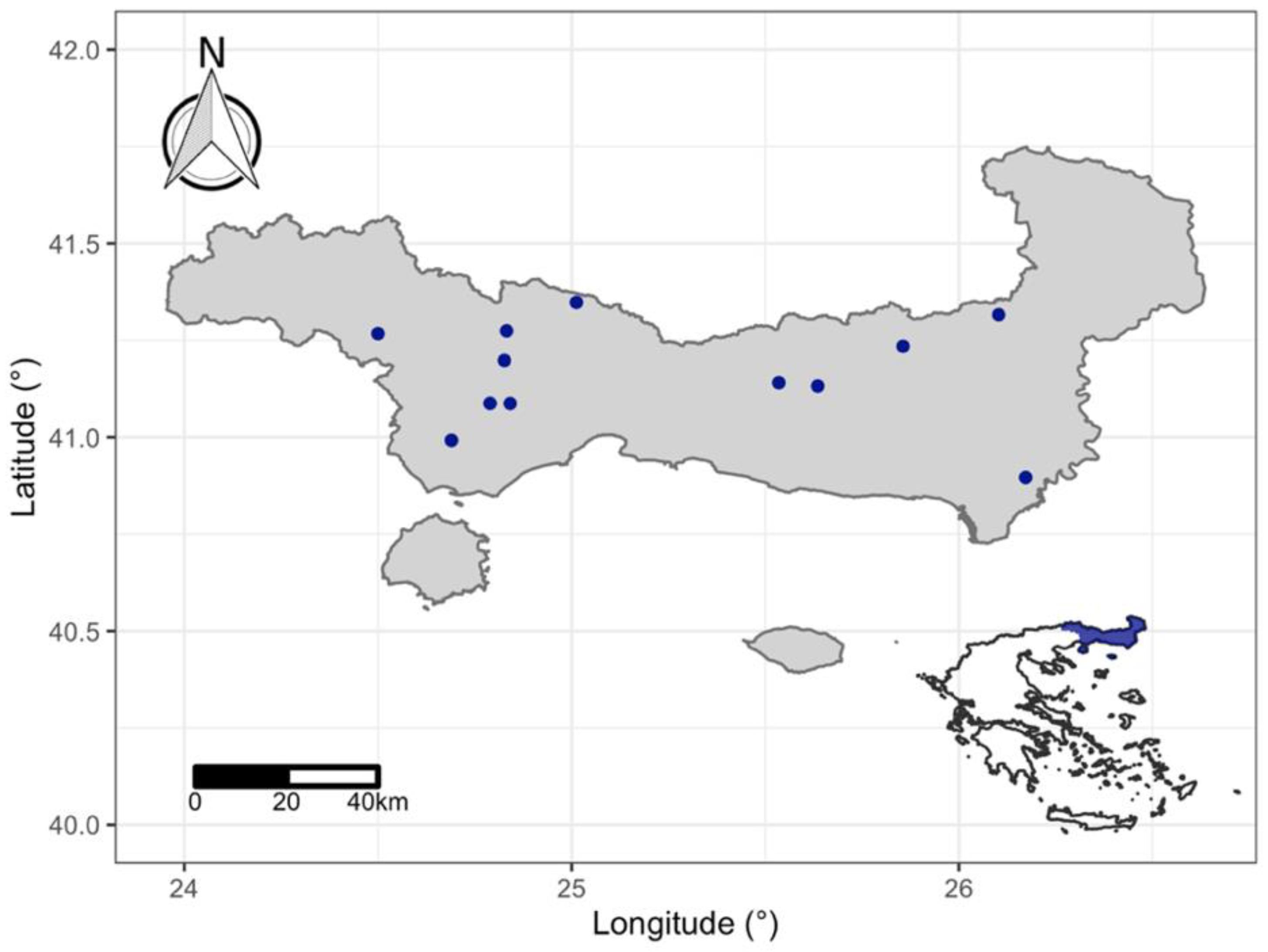
2.1. Data Acquisition and Processing

The study region, located to the north-east of Greece (Figure 1), extends to an area of 11,243 km² that covers the Water District of Thrace. It is delimited by the boundaries of Greece with Bulgaria and Turkey on the north and east, respectively, by the Thracian Sea on the south, and by the watershed of Nestos River on the west. This area was identified: (a) To have common rainfall erosivity spatiotemporal patterns [3]; (b) to form a region with a distinct monthly temporal distribution of erosivity density [13], a parameter strongly related to seasonal rainfall intensity [10]; and (c) to have similar intra-storm temporal distribution intensity patterns of heavy and, consequently, erosive precipitation [22].

Pluviograph data for 12 meteorological stations were taken from the Greek National Bank of Hydrological and Meteorological Information (NBHM) [23]. The time series comprised a total of 372 years of pluviograph records with a time step of 30 min for the time period from 1965 to 1996 (

Table 1. Meteorological station locations and record data durations.

	Name	Latitude (°)	Longitude (°)	Elevation (m)	Duration (y)
1	TOXOTES	41.09	24.79	75	27
2	M. DEREIO	41.32	26.10	116	22
3	FERRES	40.90	26.17	43	31
4	PARANESTI	41.27	24.50	122	34
5	GRATINI	41.14	25.53	120	27
6	KECHROS	41.23	25.86	700	24
7	M. KSIDIA	41.13	25.64	70	27
8	THERMES	41.35	25.01	440	26
9	GERAKAS	41.20	24.83	308	24
10	ORAIO	41.27	24.83	656	26
11	SEMELH	41.09	24.84	65	23
12	CHRYSOUPOLI	40.99	24.69	15	14

). The time series rainfall records were checked for consistency and cleared from errors.

2.2. Rainfall Erosivity Calculations

The erosivity of a single erosive rainfall event, $E{I}_{30}$ (MJ·mm/ha/h), was computed using the pluviograph records [1]:

$$E{I}_{30}=\left({\displaystyle \sum }_{r=1}^m{e}_r\cdot v_r\right)\cdot I_{30}$$

(1)

where $e_r$ is the kinetic energy per unit of rainfall (MJ/ha/mm), $v_r$ the rainfall depth (mm) for the time interval $r$ of the hyetograph, which has been divided into $r=1,2,\dots ,m$ time sub-intervals, and $I_{30}$ is the maximum rainfall intensity for a 30 min duration during that rainfall.

The quantity $e_r$ was calculated for each time sub-interval, $r$, applying the kinetic energy equation used in RUSLE2 [10]:

$$e_r=0.29\left(1-0.72e^{-0.82i_r}\right)$$

(2)

where $i_r$ is the rainfall intensity (mm/h).

An individual rainfall event was extracted from the continuous pluviograph data, if its cumulative depth for a duration of 6 h at a certain location was less than 1.27 mm. A rainfall event was considered to be erosive if it had a cumulative rainfall depth greater than 12.7 mm. Given that the use of coarser fixed time intervals as 30 min to a finer one can lead to an underestimation of the value of erosivity, the appropriate monthly conversion factors, previously computed for Greece [3], were applied.

The daily erosivity $R_d$ (MJ·mm/ha/h/d) was either set equal to the sum of all daily events or when a storm was crossed temporally by two or more consecutive days; it was assigned to the first calendar day:

$$R_d={{\displaystyle \sum }}_{i=1}^n{\left(E{I}_{30}\right)}_i$$

(3)

where $i=1,...,n$ are the erosive events that initiate during calendar day d.

2.3. Empirical Equations for the Estimation of Erosivity

The empirical equations utilized were the Richardson et al. [24] and the Yu and Rosewell [25] models, which are given in Equations (4) and (5), respectively:

$$R_{d, Rich}={\alpha }_{m,s}\cdot P_d^{{\beta }_{m,s}}$$

(4)

where $R_{d, Rich}$ is the daily erosivity, $P_d$ is the daily precipitation, and the parameters ${\alpha }_{m,s}$ and ${\beta }_{m,s}$ correspond to station s and month m.

$$R_{d, Yu}={\alpha }_s\cdot \left[1+{\beta }_s\cdot cos\left(\frac{\pi }{6}m-\omega \right)\right]P_d^{{\gamma }_s}$$

(5)

where $R_{d, Yu}$ is the daily erosivity; the parameters ${\alpha }_s$, ${\beta }_s$, and ${\gamma }_s$ are different for every station s; $m$ is the month; and ω is the month with the highest average daily erosivity values. The parameters in the previous equations were determined using nonlinear least squares as implemented in the R language package stats [26].

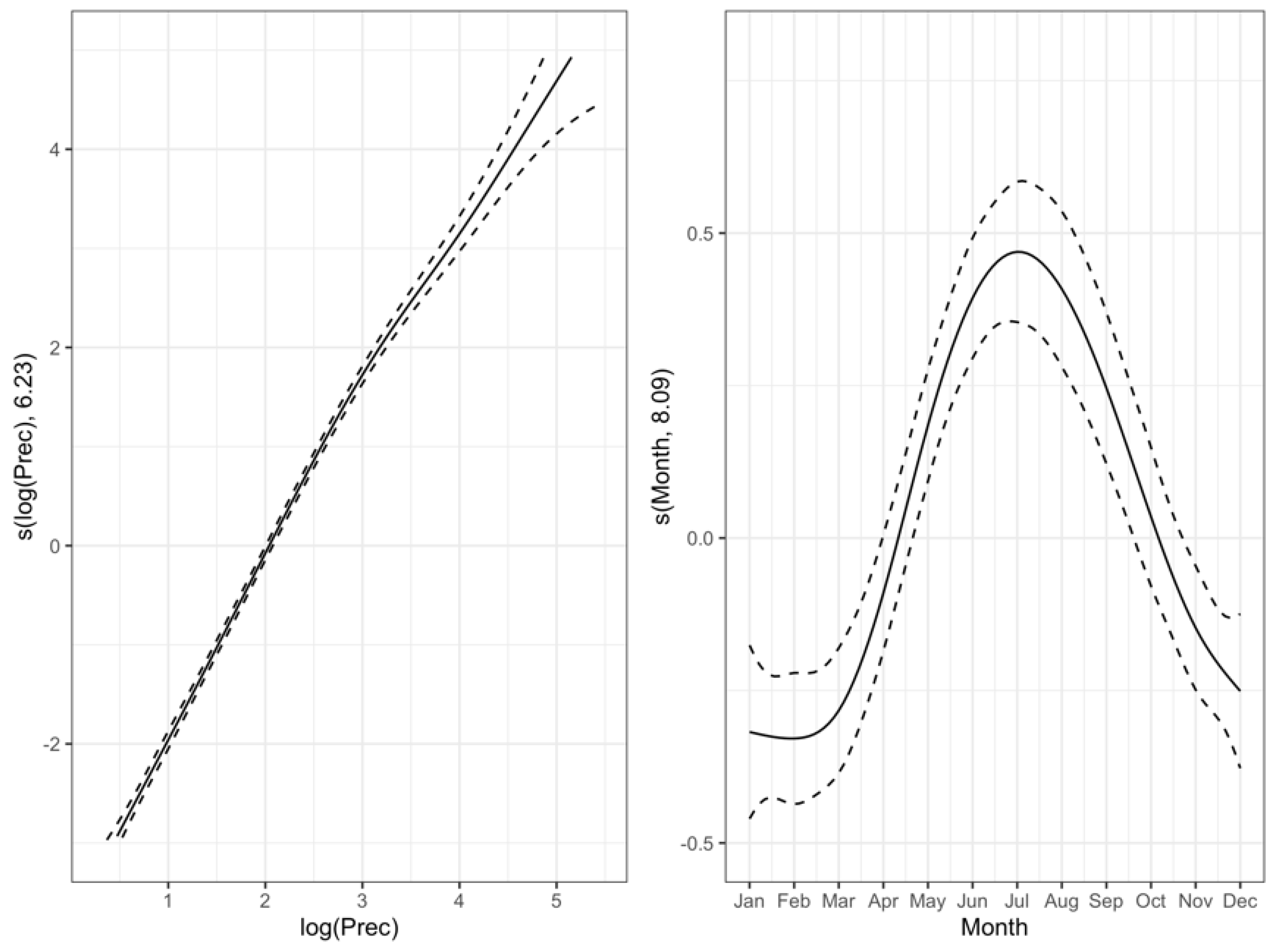
2.4. Generalized Aditive Models

As previously mentioned, GAMs provide a generic framework for the extension of GLM and were introduced by Hastie and Tibshirani [16]. A GLM has the form [27]:

$$g(E(Y|X)=\beta \bullet X$$

(6)

where g(.) is a link function, a priori known, that transforms the output response $Y$ in order to make the model linear; $Y$ is expected to follow a distribution from the exponential family; $\beta$ is a vector of unknown parameters; and X is the matrix of input variables.

A GAM usually has the form [16]:

$$g(E(Y|X)=\alpha +{{\displaystyle \sum }}_{j=1}^m{f}_j\left(x_j\right)$$

(7)

where $\alpha$ is the intercept and $f_j$ is the smooth function, called the “smooth,” of the j-th input variable $x_j$. Smooths consist of a set of basis functions [28]:

$$f\left(x\right)={{\displaystyle \sum }}_{i=1}^n{b}_i\left(x\right)\bullet {\beta }_i$$

(8)

where $b_i$ is the basis function and ${\beta }_i$ are unknown parameters. Some indicative basis functions that are used are polynomial, cubic, or penalized regression splines, or thin-plate regression splines. Computationally efficient fitting procedures have been developed and implemented in the open source R language packages gam [29] and mcgv [28], which automatically select the smoothing parameters.

The reader can find more details about alternative fitting algorithms in [15,18,30,31,32].

In this paper, a GAM model was fitted using the daily erosivity as an output response, and the smooths of the logarithm of daily precipitation and the smooth of the month as numerical values (1,2..,12) as input variables. The basis function was penalized thin-plate regression splines. A log link function was used and daily erosivity was assumed to be distributed according to the Gamma distribution as positive and highly skewed [12,33,34].

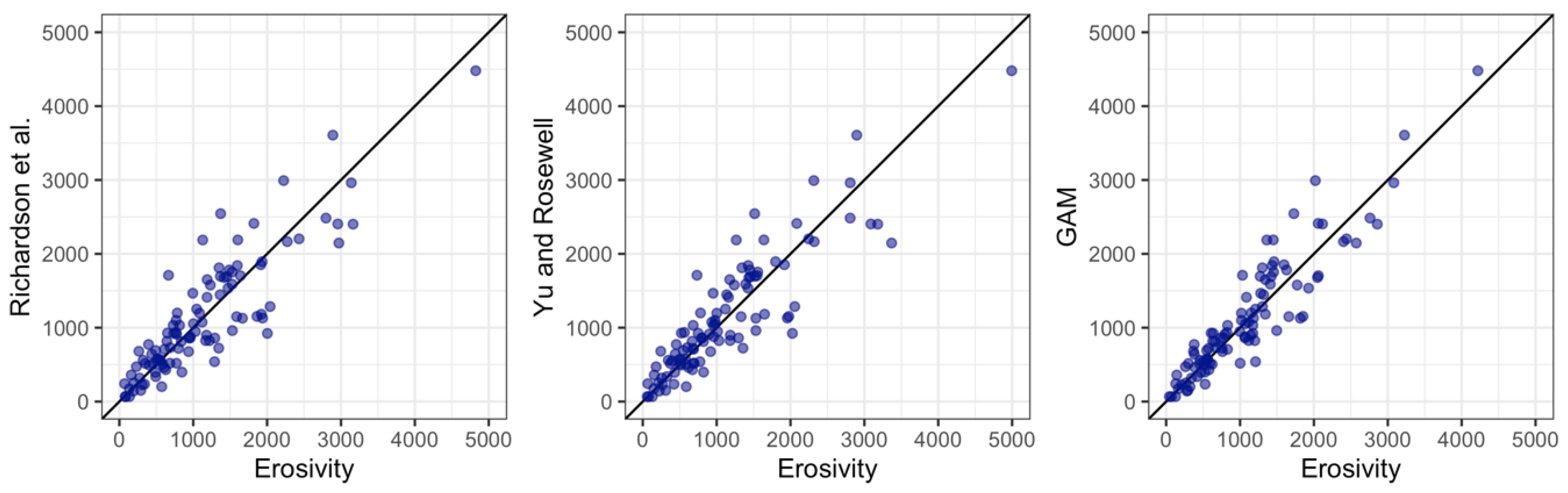
2.5. Validation and Model Performance Criteria

The daily aggregated data were divided using 70% of them as a training set and 30% as testing. The split was based on the years that constitute the dataset. In this way, it was made possible to estimate the out-of-sample error of the models on new data using both the initial daily step of the dataset and a further aggregated annual, based on daily estimates, in order to examine the presence of systematic errors, as previous studies reported systematic underestimation [12,34]. As measures of the out-of-sample error on the test set, the coefficient of determination $R^2$, the root-mean-squared error (RMSE), and the mean absolute error (MAE) were used:

$$R^2=1-\frac{{{\displaystyle \sum }}_{i=1}^m{\left(\widehat{y_i}-y_i\right)}^2}{{{\displaystyle \sum }}_{i=1}^m{\left(\widehat{y_i}-{\mu }_y\right)}^2}$$

(9)

$$RMSE=\sqrt{\frac{1}{m}{\displaystyle \sum }_{i=1}^m{\left(\widehat{y_i}-y_i\right)}^2}$$

(10)

$$MAE=\frac{1}{m}{\displaystyle \sum }_{i=1}^m\left|\widehat{y_i}-y_i\right|$$

(11)

where $m$ is the number of the samples in the test set (daily or annual), $\widehat{y_i}$ is the predicted value of $y_i$ that belongs in the test set, and ${\mu }_y$ is the mean of $y_i$. $R^2$ describes the ratio of variance that is explained by a model and may be negative, among other reasons, if an inappropriate model is used [35].

3. Results and Discussion

The daily dataset consisted of 10,424 records for all the stations. Using the training set: (a) the empirical equations, Equations (4) and (5), were fitted for each station; (b) a single GAM was fitted using all stations’ data, representative of the area. Figure 2 illustrates the partial effect plots of the smoothing functions used in the GAM model. Precipitation had a monotonic nonlinear effect and the month a smooth seasonal pattern, with its maximum during summer. Both smoothing functions add to the overall prediction of erosivity.

The reported estimated degrees of freedom (>>1) indicated nonlinear smoothing functions. The computed approximate significance p-values of both smooth terms was less than 10⁻¹⁶ and the deviance explained by the model was 86.5% (in the training set). Given the above values, there was strong evidence that both terms explained erosivity adequately.

The comparison of the models was based on their error metrics on the test set using daily and annual time steps. These results are given in

Table 2. Annual time step estimation of the out-of-sample error metrics for the two empirical equations and GAM. R² values are unitless. Root-mean-squared error (RMSE) and mean absolute error (MAE) values are in MJ·mm·ha⁻¹h⁻¹y⁻¹.

Model	R2	RMSE	MAE
GAM	0.88	306.43	231.20
Richardson et al.	0.77	419.64	308.50
Yu and Rosewell	0.76	431.19	309.24

and

Table 3. Daily time step estimation of the out-of-sample error metrics for the two empirical equations and GAM. R² values are unitless. RMSE and MAE values are in MJ·mm·ha⁻¹h⁻¹.

Model	R2	RMSE	MAE
GAM	0.73	89.19	53.00
Richardson et al.	0.63	104.83	61.28
Yu and Rosewell	0.61	107.58	59.82

, where the single GAM performed better than those of the fitted parametric equations (R² was closer to one, and RMSE and MAE had lower values).

Figure 3 depicts the annual erosivity values as calculated in the test set versus the values estimated from the three models. In these two diagrams, the GAM’s estimations present less scatter than those coming from the empirical equations. In addition, all methods did not systematically underestimate R values.

4. Conclusions

In summary, this paper presented an indicative sample of the use of the GAM in the problems associated with the estimation of erosivity using daily precipitation values. These coarser precipitation data are in abundance worldwide, in contrast to pluviograph values that are required for the calculation of erosivity. Through the use of GAM, it became possible to model the nonlinear relationships in an additive way between rainfall erosivity, the daily rainfall, and seasonal periodicity. Using 30% of the data as an independent test set, just one model gave erosivity estimates with a significantly smaller error on a daily and on a yearly basis, utilizing the sums of the daily values, in comparison to the estimates from the application of two well-known nonlinear empirical equations, which were applied for every station, using data from the Greek Water District of Thrace.

References

1. Nearing, M.A.; Yin, S.; Borrelli, P.; Polyakov, V.O. Rainfall erosivity: An historical review. Catena 2017, 157, 357–362. [Google Scholar] [CrossRef]
2. Li, Z.; Fang, H. Impacts of climate change on water erosion: A review. Earth-Sci. Rev. 2016, 163, 94–117. [Google Scholar] [CrossRef]
3. Vantas, K.; Sidiropoulos, E.; Loukas, A. Estimating Current and Future Rainfall Erosivity in Greece Using Regional Climate Models and Spatial Quantile Regression Forests. Water 2020, 12, 687. [Google Scholar] [CrossRef]
4. Geeson, N.A.; Brandt, C.J.; Thornes, J.B. Mediterranean Desertification: A Mosaic of Processes and Responses; John Wiley & Sons: West Sussex, UK, 2003. [Google Scholar]
5. Griggs, D.; Stafford-Smith, M.; Gaffney, O.; Rockström, J.; Öhman, M.C.; Shyamsundar, P.; Steffen, W.; Glaser, G.; Kanie, N.; Noble, I. Sustainable development goals for people and planet. Nature 2013, 495, 305–307. [Google Scholar] [CrossRef]
6. Boardman, J.; Poesen, J. Soil Erosion in Europe: Major Processes, Causes and Consequences. In Soil Erosion in Europe; John Wiley & Sons: Wiltshire, UK, 2006; pp. 477–487. ISBN 10-0-470-85910-5. [Google Scholar]
7. Renard, K.G.; Freimund, J.R. Using monthly precipitation data to estimate the R-factor in the revised USLE. J. Hydrol. 1994, 157, 287–306. [Google Scholar] [CrossRef]
8. Wischmeier, W.H.; Smith, D.D. Predicting Rainfall Erosion Losses-a Guide to Conservation Planning; USDA, Agriculture Handbook No. 537; Government Printing Office: Washington, DC, USA, 1978.
9. Renard, K.G.; Foster, G.R.; Weesies, G.A.; Porter, J.P. RUSLE: Revised universal soil loss equation. J. Soil Water Conserv. 1991, 46, 30–33. [Google Scholar]
10. USDA-ARS. Science Documentation: Revised Universal Soil Loss Equation, Version 2 (RUSLE 2); USDA-Agricultural Research Service: Washington, DC, USA, 2013.
11. Borrelli, P.; Alewell, C.; Alvarez, P.; Anache, J.; Baartman, J.E.M.; Ballabio, C.; Bezak, N.; Biddoccu, M.; Cerdà, A.; Chalise, D.; et al. Soil erosion modelling: A global review and statistical analysis. 2020; Submitted for publication. [Google Scholar]
12. Vantas, K.; Sidiropoulos, E.; Evangelides, C. Rainfall Erosivity and Its Estimation: Conventional and Machine Learning Methods. Soil Eros. 2019. [Google Scholar] [CrossRef]
13. Vantas, K.; Sidiropoulos, E.; Loukas, A. Robustness Spatiotemporal Clustering and Trend Detection of Rainfall Erosivity Density in Greece. Water 2019, 11, 1050. [Google Scholar] [CrossRef]
14. Vantas, K.; Sidiropoulos, E. Imputation of erosivity values under incomplete rainfall data by machine learning methods. Eur. Water 2017, 57, 193–199. [Google Scholar]
15. Friedman, J.; Hastie, T.; Tibshirani, R. The Elements of statistical Learning; Springer: New York, NY, USA, 2001; Volume 1. [Google Scholar]
16. Hastie, T.J.; Tibshirani, R.J. Generalized Additive Models. Stat. Sci. 1986, 1, 297–318. [Google Scholar] [CrossRef]
17. James, G.; Witten, D.; Hastie, T.; Tibshirani, R. An Introduction to Statistical Learning; Springer: Berlin/Heidelberg, Germany, 2013; Volume 112. [Google Scholar]
18. Wood, S.N.; Pya, N.; S"afken, B. Smoothing parameter and model selection for general smooth models (with discussion). J. Am. Stat. Assoc. 2016, 111, 1548–1575. [Google Scholar] [CrossRef]
19. Ouarda, T.B.M.J.; Charron, C.; Hundecha, Y.; St-Hilaire, A.; Chebana, F. Introduction of the GAM model for regional low-flow frequency analysis at ungauged basins and comparison with commonly used approaches. Environ. Model. Soft. 2018, 109, 256–271. [Google Scholar] [CrossRef]
20. Garcia Galiano, S.G.; Olmos Gimenez, P.; Giraldo-Osorio, J.D. Assessing Nonstationary Spatial Patterns of Extreme Droughts from Long-Term High-Resolution Observational Dataset on a Semiarid Basin (Spain). Water 2015, 7, 5458–5473. [Google Scholar] [CrossRef]
21. Shortridge, J.E.; Guikema, S.D.; Zaitchik, B.F. Machine learning methods for empirical streamflow simulation: a comparison of model accuracy, interpretability, and uncertainty in seasonal watersheds. Hydrol. Earth Syst. Sci. 2016, 20, 2611–2628. [Google Scholar] [CrossRef]
22. Vantas, K.; Sidiropoulos, E.; Vafeiadis, M. Optimal temporal distribution curves for the classification of heavy precipitation using hierarchical clustering on principal components. Glob. NEST J. 2019, 21, 530–538. [Google Scholar]
23. Vantas, K. hydroscoper: R interface to the Greek National Data Bank for Hydrological and Meteorological Information. J. Open Source Soft. 2018, 3, 625. [Google Scholar] [CrossRef]
24. Richardson, C.; Foster, G.; Wright, D. Estimation of erosion index from daily rainfall amount. Trans. ASAE 1983, 26, 153–156. [Google Scholar] [CrossRef]
25. Yu, B.; Rosewell, C. An assessment of a daily rainfall erosivity model for New South Wales. Soil Res. 1996, 34, 139–152. [Google Scholar] [CrossRef]
26. R Core Team. R: A Language and Environment for Statistical Computing; R Core Team: Vienna, Austria, 2019. [Google Scholar]
27. Nelder, J.A.; Wedderburn, R.W.M. Generalized Linear Models. J. R. Stat. Soc. Ser. Gen. 1972, 135, 370. [Google Scholar] [CrossRef]
28. Wood, S.N. Generalized Additive Models: An Introduction with R, 2nd ed.; Chapman and Hall/CRC: New York, NY, USA, 2017. [Google Scholar]
29. Hastie, T. gam: Generalized Additive Models. 2020. Available online: https://CRAN.R-project.org/package=gam (accessed on 10 May 2020).
30. Hastie, T.J.; Tibshirani, R.J. Generalized Additive Models; CRC press: Boca Raton, FL, USA, 1990; Volume 43. [Google Scholar]
31. Wood, S.N. Fast stable restricted maximum likelihood and marginal likelihood estimation of semiparametric generalized linear models. J. R. Stat. Soc. B 2011, 73, 3–36. [Google Scholar] [CrossRef]
32. Breiman, L.; Friedman, J.H. Estimating Optimal Transformations for Multiple Regression and Correlation. J. Am. Stat. Assoc. 1985, 80, 580–598. [Google Scholar] [CrossRef]
33. Vantas, K. Determination of Rainfall Erosivity in the Framework of Data Science Using Machine Learning and Geostatistics Methods; Aristotle University of Thessaloniki: Thessaloniki, Greece, 2017. [Google Scholar]
34. Beguería, S.; Serrano-Notivoli, R.; Tomas-Burguera, M. Computation of rainfall erosivity from daily precipitation amounts. Sci. Total Environ. 2018, 637–638, 359–373. [Google Scholar] [CrossRef] [PubMed]
35. Kvålseth, T.O. Cautionary note about R2. Am. Stat. 1985, 39, 279–285. [Google Scholar]
36. Vantas, K. Hyetor: R Package to Analyze Fixed Interval Precipitation Time Series. 2020. Available online: https://github.com/kvantas/hyetor (accessed on 10 May 2020).
37. Wickham, H. Ggplot2: Elegant Graphics for Data Analysis; Springer: New York, NY, USA, 2016. [Google Scholar]
Figure 1. Station locations used in the analysis in the Greek Water District of Thrace.
Environsciproc 02 00021 g001
Figure 2. Plots of the smoothing functions of each variable used in generalized additive models (GAMs). Dashed lines give the confidence intervals of the predictions of the fitted smooth curves (solid lines). The number in the parenthesis (Y-axis) gives the estimated degrees of freedom for the model terms.
Environsciproc 02 00021 g002
Figure 3. Calculated annual erosivity values coming from pluviograph data, versus predicted values using the three models on the testing set. The black line symbolizes the identity function f(x) = x. Values are in MJ·mm·ha−1h−1.
Environsciproc 02 00021 g003