Upstream Propagating Long-Wave Modes at a Microtidal River Mouth ^†

Abstract

We illustrate recent findings on the upriver propagation of long waves entering the mouth of the Misa River (Senigallia, Italy). Such a microtidal environment has been recently studied to understand river–sea interactions: it has been found that the river forcing dominates over the marine actions in winter, especially during storms. However, upriver wave propagation is not negligible with low-frequency waves propagating upriver for distances of the order of kilometers. With the aim to better understand the behavior of low-frequency waves propagating upriver, the analysis of the present work builds on field data collected by instruments installed close to the mouth and along the final reach of the Misa River: a tide gauge, two hydrometers and an acoustic Doppler sensor. It has been here observed that the tidal forcing (periods of the order of hours/days) is significantly strong at a distance of more than one kilometer from the river mouth, while shorter waves, like seiches (periods of some hours), are less important and are supposed to largely dissipate at the estuary, although their role could be of importance during relatively short events (e.g., floods).

1. Introduction

Estuarine environments are dynamically complex, with the hydrodynamics being triggered by many factors, e.g., nonlinear interactions between the bathymetry, the river current and many sea forcing actions [1,2]. The sediment transport and related morphodynamics derive from such complexity and act in the estuarine region by shaping the river bed and sometimes leading to interesting morphological features, like river mouth bars that after being generated, migrate and evolve in proximity of the river mouth [3].

In recent decades, important efforts have been spent towards the understanding of the evolution of infragravity (IG hereafter) waves, a specific type of low-frequency waves characterized by periods smaller than those related to sea/swell waves. Some literature works take this interval as constant, others make this depend on the peak frequency given by gravity wind waves. These can be generated, e.g., as group bound long waves, or from swell–swell interactions [4,5,6]. The importance of such waves on the sediment transport in the nearshore is also widely documented, e.g., [7].

In this context, a series of field studies has been recently carried out to better understand the wave propagation within the microtidal estuary and final reach of the Misa River (MR hereafter), located in the municipality of Senigallia (Marche Region, Italy) and flowing into the middle Adriatic Sea [8,9,10]. Two experimental campaigns were undertaken in September 2013 and January 2014, aiming at characterizing the main forcing actions interacting in the estuarine region. The data analysis showed that summertime is mainly characterized by calm periods and relatively mild storms, during which the wind continuously changes its direction and waves are relatively low. Conversely, wintertime is featured by alternating calm and severe storm events characterized by almost constant wind directions and high waves. Such behavior and seasonal differences underline a strong interaction between sea/swell waves, tide and river current during winter storms, which promotes large mixing and shear within the water column in the estuarine area [8,9]. Moreover, one of the observed winter storms well penetrated within the MR was characterized by a direction almost perpendicular to the MR mouth. This led to an upriver propagation of all wave components during the storm, especially the IG band, while the sea/swell components experienced a large breaking-induced decay at the mouth [10]. Sediment samples and water-surface elevations recorded along the MR also suggested an upriver propagation of the tidal forcing up to distances larger than ~2 km from the estuary [9].

The present work investigates further the role of long-wave propagation within the MR, mainly focusing on frequencies that are smaller or comparable to those associated with the IG band. This is correlated to the peak frequency of the wave spectral density, and a recent analysis of storm conditions in the Adriatic Sea used the IG band (0.0016–0.05) Hz [10], in agreement with other literature studies [11].

The case study is presented in Section 2. The main results, coming from a series of sensors installed within the MR, are discussed in Section 3. The final section closes the manuscript.

2. Case Study: Misa River Estuary

The study site is at the final reach of the MR, which flows from the Appennine mountains to the Adriatic Sea, its estuary being located in the municipality of Senigallia (Ancona, Italy). The MR watershed is about 383 km² and a discharge of ~400 m³/s is associated with a return period of 100 years, while the estuary is classified as microtidal, with tidal excursion not larger than 50 cm. The river shows a low-flow regime in summertime, while a relatively large surface flow characterizes the wintertime with a large dominance of the river forcing on both wave and tidal actions [8,9]. In addition, the river mouth acts as a low-pass filter, by letting low-frequency waves enter the channel, whereas higher frequency oscillations, like swell waves, are blocked. IG waves have been observed to propagate upriver with velocities up to (3–5) m/s, according to the tidal excursion in the river [10].

In the present work, the final 10 km-long stretch of the MR is analyzed, with a focus on the data collected by two hydrometers, property of the Civil Protection (Marche Region), and an acoustic sensor, installed within the framework of the MORSE (“Modeling and Observation of River–Sea Exchanges”) project, funded by the Office of Naval Research—Global (UK). The hydrometers measure every 30 min only the water surface level and are installed at two locations: “Ponte Garibaldi” (~1.5 km from the MR estuary, RG1 hereafter) and “Bettolelle” (~10 km from the MR estuary, RG2 hereafter) [10]. The acoustic sensor is a Horizontal Acoustic Doppler Current Profiler (H-ADCP) and measures every 2 min both velocity and flow rate, in addition to the water surface level. This is located at RG1, about 20 m upstream of the “Ponte Garibaldi” hydrometer. The reference level, or datum, of all instruments is chosen as the local riverbed. A tide gauge with sampling period of 6 min, located inside Senigallia harbor, is also used to provide information on tidal levels in the area.

Figure 1 illustrates the extended map of the study site (a) and a picture of the RG1 instruments (b). Data collected by such instruments between September and December 2019 are here used.

3. Results and Discussion

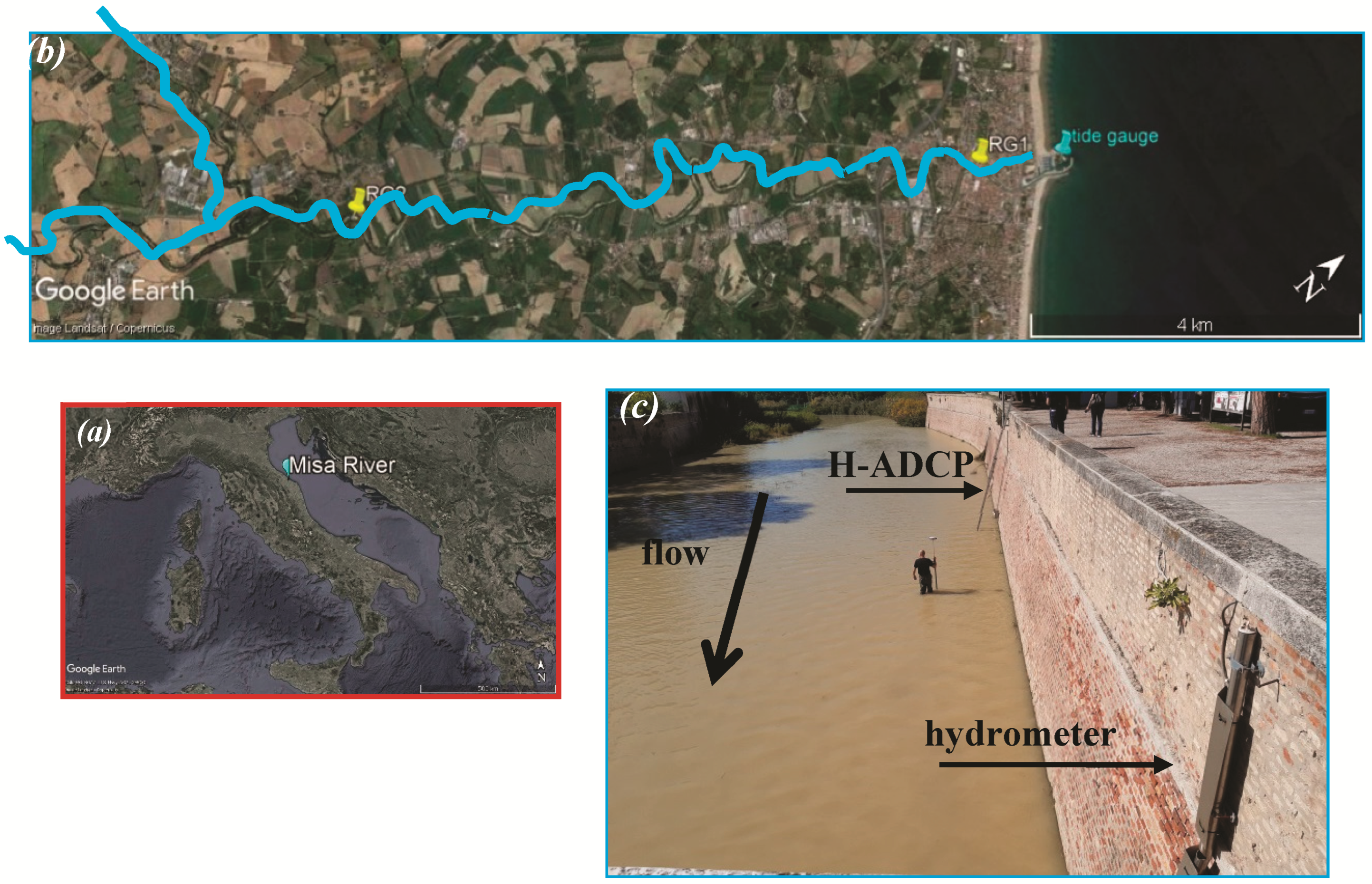
The flow in the final MR stretch is affected by many forcing actions. Specifically, the river discharge is modulated by the sea entering the estuary and propagating upriver. Hence, to give evidence of such behavior, the data collected by the sensors located at RG1, RG2 and Senigallia harbor are analyzed.

3.1. Analysis of the Collected Data

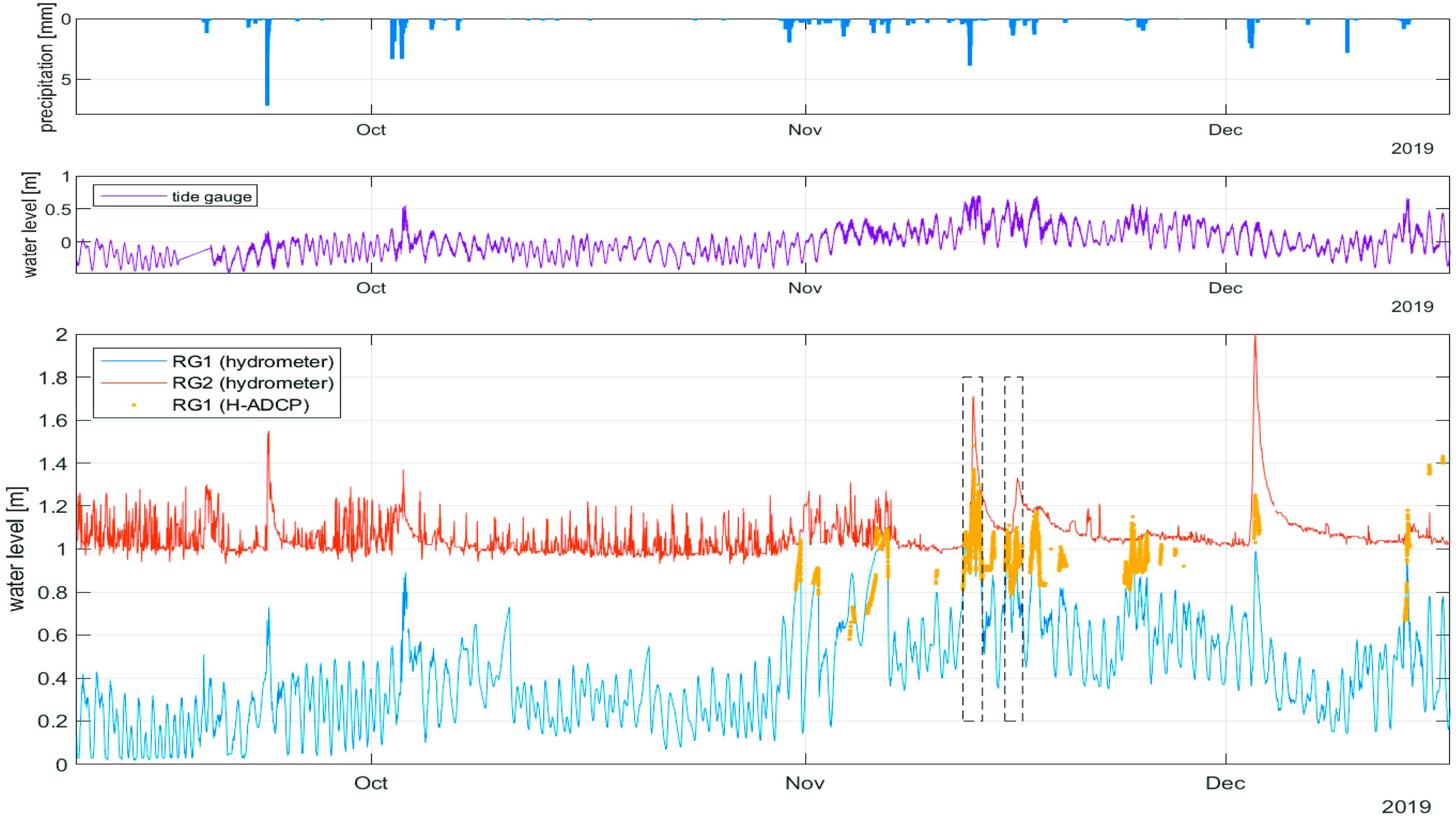
The time series of the latest events recorded between September and December 2019 are illustrated in Figure 2, where the mean precipitation level measured in the MR watershed is also shown (top panel). The tide-gauge series is shifted vertically and oscillates around the time-averaged level (middle panel). The water-level recorded by the hydrometers located at RG1 (blue line) and RG2 (red line) refer to the riverbed level, as well as the water level collected by the H-ADCP (yellow dots) at RG1 (bottom panel). Comparing the hydrometer time series, more frequent oscillations are observed at Ponte Garibaldi, where the tidal forcing is much stronger than at Bettolelle, as also visible if compared to the tide-gauge series (see also [10]). Additional peaks are observed at both locations and are fairly evident in the investigated wintertime period, especially because of the more frequent precipitations and larger runoff in the MR watershed. The main peaks correspond to the intense precipitations occurring in 23 September (15-min precipitation of about 7 mm) and 2–3 October (about 3 mm). However, such events did not lead to significantly high water levels in the MR, probably due to a relatively dry watershed in such periods. Hence, the H-ADCP was not submerged and did not provide any measure. Conversely, relatively weaker but long-lasting events (e.g., those occurring at the beginning of November) combined with more intense precipitations (~4 mm in 12 November) led to higher water levels and enabled the H-ADCP to be submerged and properly collect data.

In addition to short events that occurred between October and December 2019, a couple of relatively long events can be observed in Figure 2 (black rectangles), both lasting a bit more than one day, i.e., one between 12 and 13 November, the other between 15 and 16 November. The spectral content of these events is discussed in the following sections.

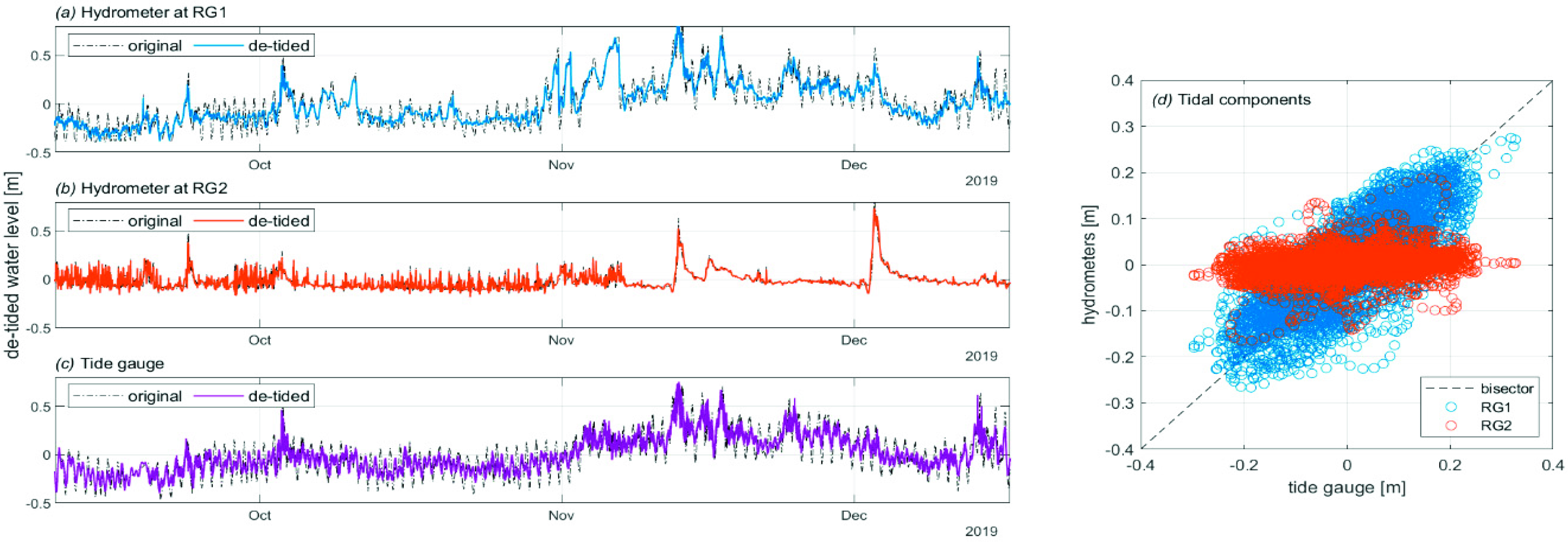
To better understand the dependence of the role of tide within the MR, Figure 3a–c illustrates both original (dash-dotted black lines) and de-tided signals, obtained by filtering out periods in the 12–24 h range (colored solid lines). Each series is vertically shifted by a quantity equal to its time average. The main difference among the recordings is that the tidal component, i.e., that related to periods in the range 12–24 h, is almost absent at RG2 (Figure 3b), with original and de-tided signals almost overlapping. Conversely, the tide plays an important role at both RG1 (Figure 3a) and harbor (Figure 3c).

The dependence of each signal on the tidal constituents can better be seen in Figure 3d, where the tidal component recorded by the tide gauge is plotted against the same component recorded by both hydrometers. The data related to the RG1 hydrometer fall around the bisector, demonstrating a strong correlation with the tidal forcing. Conversely, the tidal component recorded at RG2 distributes around zero, thus showing a weak dependence on the tidal forcing.

The influence of the sea forcing at RG1 is confirmed by the larger de-tided surface levels observed during some events, simultaneously recorded by the tide gauge, e.g., at the beginning of October, around the middle of November and the end of December (compare top and bottom panels). Conversely, the RG2 hydrometer seems to be the only one affected by more frequent perturbations, not occurring during the above-mentioned events (middle panel).

3.2. Data Comparison at RG1

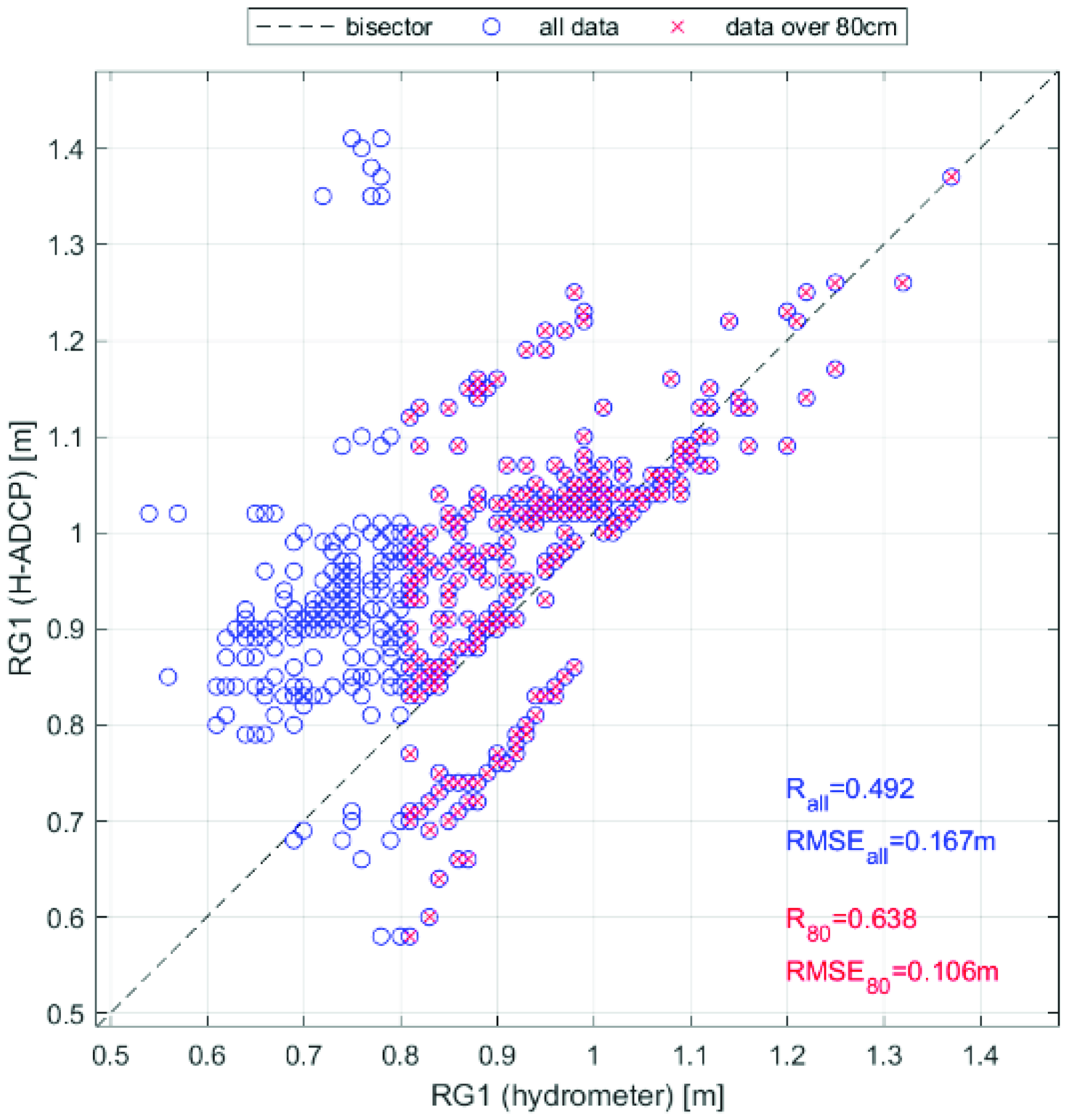
From a first inspection of Figure 2, the data collected by both instruments located at RG1 are in a relatively good agreement, with the H-ADCP sometimes providing larger values. The scatter plot of Figure 4 better illustrates the comparison. In detail, due to the difference in the sampling rate of the two instruments (2’ versus 30’), only the H-ADCP data collected simultaneously with the hydrometer have been considered. Blue circles represent the whole data sets, in agreement with the time series of Figure 2, while red crosses represent only the data referring to a water level larger than 80 cm, when the H-ADCP was completely submerged.

The correlation between the recorded signals has been evaluated using the correlation coefficient R and the RMSE coefficient. As shown in Figure 4, the reduced sample provides better performances, with the RMSE passing from 0.167 to 0.106 m and the correlation significantly increasing. The main factors that can be attributed to such difference are the distance between the sensors, e.g., the hydrometer is much closer to the bridge, with the flow being slightly different; the instrument sampling rate and the consequent difference due to the averaging performed on the H-ADCP data.

For the following spectral analysis (Section 3.3), all data falling in the chosen events (black rectangles in Figure 2) are used. In such periods, water levels smaller than 80 cm only represent 3% of the data referring to the 15–16 November event, while all recorded water levels are over 80 cm in the 12–13 November event.

3.3. Spectral Analysis

The data collected by the hydrometers located at RG1 and RG2, the H-ADCP at RG1 and the tide gauge have been analyzed from the spectral viewpoint. The main features of the spectral analysis are reported in

Table 1. Features of the spectral analysis.

	Hydrometers (RG1 and RG2)	H-ADCP (RG1) 12–13 Nov 2019	H-ADCP (RG1) 15–16 Nov 2019	Tide Gauge
Degree of freedom [-]	35	6	6	21
Frequency interval [Hz]	2.2 × 10−6	3.3 × 10−5	3.3 × 10−5	1.4 × 10−6
Segment length [hours]	2352.00	33.33	30.23	2615.15

.

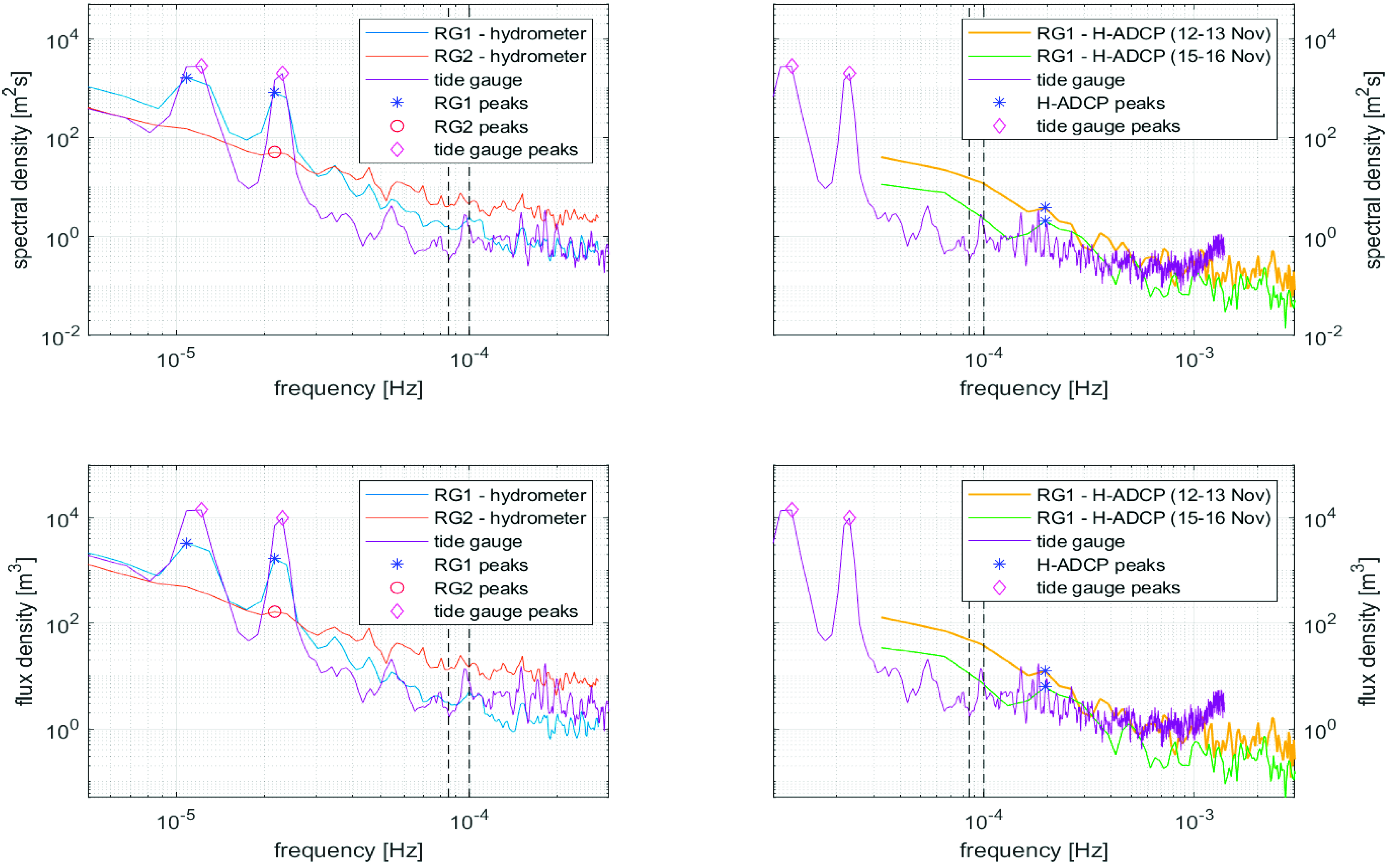
Both spectral density and flux density, the latter being the product between the spectral density and the group velocity, are illustrated in Figure 5, respectively, in the top and bottom panels. Due to the different sampling rates of the instruments in use and to better illustrate the spectral features of each of them, the x-axis limits have been adapted either to the hydrometer data (left panels) or to the H-ADCP data (right panels). Further, for comparison purposes, the spectral response of the tide gauge is illustrated in all panels.

The left panels refer to the hydrometer and tide-gauge data recorded between 10 September and 17 December 2019. The spectral behavior of both hydrometers is qualitatively similar in the lower reach of the spectra, i.e., for frequencies f > 0.5 × 10⁻⁴ Hz. However, a larger spectral density is observed at RG2, this being likely due to typical high-frequency oscillations occurring at more inland locations, where short-period perturbations are much more frequent than downstream. These are mainly due to a more irregular riverbed, a larger bed roughness and a steeper slope, all leading to a larger turbulence and to an intensity increase of high-frequency modes. On the other hand, significant differences are observed at smaller frequencies (f < 0.5 × 10⁻⁴ Hz). Peak values in both flux and spectral densities are more evident at RG1 (colored symbols), with peak frequencies referring to diurnal (~25.6 h) and semi-diurnal (~12.8 h) tidal constituents. At RG2, only the semidiurnal constituent exists, although its contribution is significantly poor. A comparable spectral density is obtained from the tide-gauge series, which again shows the highest peaks in correspondence with the diurnal and semi-diurnal tidal constituents, thus reinforcing the large importance of the tide both close to the coast (harbor) and 1 km inland of the river mouth (RG1).

An additional analysis (not shown here), performed using a reduced degree of freedom, shows a large amount of spectral density corresponding to periods around 30–40 days, which explains the oscillation observed in Figure 2, evident for both the RG1 hydrometer and the tide gauge. Here, an increasing trend of the water level occurs between the end of October and November, while a decreasing trend characterizes the final part of November and the beginning of December.

The right panels of Figure 5 represent both spectral and flux densities of two events recorded by the H-ADCP, located at RG1. These have been selected as the longest occurred in the investigated time range, and refer to 12–13 November (yellow lines) and 15–16 November (green lines), when both a significant amount of precipitation occurred and the river level at Ponte Garibaldi was high enough to submerge the H-ADCP (see also Figure 2). Figure 5 illustrates a large spectral contribution at relatively low frequencies, with the highest local peak corresponding to about 1.42 h (blue asterisks). Typical tidal constituents are smaller than the used frequency limits and cannot be individuated due to the reduced duration of the recorded events.

The analysis of Figure 5 seems to suggest that a contribution may come from modes associated with the geometry of the Adriatic Sea basin, like the seiching motion. This characterizes enclosed and semi-enclosed basins and can be described through the following equation

T_seiche,n = 2L/[n(gh)^1/2],

(1)

where T_seiche,n gives the natural periods of the seiche at a specific mode n, while L is the length of the basin, h the average depth of the basin, and g the gravity acceleration. The main modes in the Adriatic Sea are characterized by periods of 21.2 h, 10.7 h and 6.7 h, usually triggered by the Scirocco wind [12,13]. However, if one wants to account for the transversal seiche motion, shorter periods are found. Specifically, in the considered study site, the distance between Senigallia and the opposite coast of the Croatian islands is L ~ 130 km. Since the depth along such distance is in the range h = (50–70) m, the mode-1 transversal seiche motion is characterized by a period T_seiche,1 = (2.8–3.3) h, i.e., by a frequency f_seiche = (0.85–1.0) × 10⁻⁴ Hz. Such frequencies fall in the descending limbs of the curves (see intervals between black dashed lines in Figure 5) for both hydrometers (left panels) and H-ADCP (right panels). In such ranges, the spectral density for the hydrometers is of order O(1–10) m²s (top left), in agreement with the events recorded by the H-ADCP, characterized by a spectral density of O(1–10) m²s (top right), but no peaks are observed, i.e., transversal seiching seems not to be perceived. Conversely, some peaks are observed in the tide-gauge series just outside the f_seiche region, i.e., at 0.54 × 10⁻⁴ Hz (left of f_seiche region) and 0.96 × 10⁻⁴ Hz (right of f_seiche region). This suggests a much more evident effect of the mode-1 seiching motion within the harbor, if compared to the effect within the MR, recorded by both hydrometers and H-ADCP.

On the other hand, the analysis of mode 2 leads to seiche periods in the range T_seiche,2 = (1.38–1.63) h, which is consistent with the local peak observed at RG1 and corresponding to 1.42 h (right panels of Figure 5). This can be seen as the possible explanation for the transversal oscillation of the Adriatic basin, which can be detected by means of high-frequency recordings during flood conditions of relatively small duration.

Such analysis reveals that perturbations characterized by the same frequency of the seiching motion are not particularly significant in the long term in the river, when tidal components are much more important, but in a relatively short term (order of hours to days), their contribution is important. Hence, the upriver propagation of seiches cannot be neglected.

Finally, the tide-gauge spectral density increases at frequencies f = (1.2–1.4) × 10⁻³ Hz and is larger than that observed at RG1. Such frequency range corresponds to periods of 12–14 min, probably related to the harbor resonance.

4. Conclusions

The present contribution illustrates some results coming from the analysis of recent data collected by instruments located along the MR and in the harbor close to the river estuary. Oscillations related to diurnal and semi-diurnal tidal constituents, as well as longer oscillations (order of months), are observed within the MR, at about 1 km from the estuary (RG1) during September-December 2019, while these do not exist at about 10 km inland (RG2).

Higher-frequency modes, with periods around 1.42 h, are also observed at RG1, which probably indicate the existence of transversal (mode-2) seiche motions within the river at RG1. This is important during stormy events, while the tidal action seems to be overwhelming during calm conditions. Future analyses will be undertaken to better understand such behavior.

Finally, data collected within the harbor show that, in addition to diurnal and semidiurnal tidal constituents, an important role is played by oscillations with periods of 12–14 min, probably due to the harbor resonance.

References

1. Dodet, G.; Bertin, X.; Bruneau, N.; Fortunato, A.B.; Nahon, A.; Roland, A. Wave-current interactions in a wave-dominated tidal inlet. J. Geophys. Res. Oceans 2013, 118, 1587–1605. [Google Scholar] [CrossRef]
2. Olabarrieta, M.; Geyer, W.R.; Kumar, N. The role of morphology and wave-current interaction at tidal inlets: An idealized modeling analysis. J. Geophys. Res. Oceans 2014, 119, 8818–8837. [Google Scholar] [CrossRef]
3. Melito, L.; Postacchini, M.; Sheremet, A.; Calantoni, J.; Zitti, G.; Darvini, G.; Brocchini, M. Wave-Current Interactions and Infragravity Wave Propagation at a Microtidal Inlet. Proceedings 2018, 2, 628. [Google Scholar] [CrossRef]
4. Symonds, G.; Huntley, D.A.; Bowen, A.J. Two-dimensional surf beat: Long wave generation by a time-varying breakpoint. J. Geophys. Res. Oceans 1982, 87, 492–498. [Google Scholar] [CrossRef]
5. Herbers, T.H.C.; Elgar, S.; Guza, R.T. Generation and propagation of infragravity waves. J. Geophys. Res. Oceans 1995, 100, 24863–24872. [Google Scholar] [CrossRef]
6. Xavier, B.; de Bakkera, A.; Apvan, D.; Giovanni, C.; Gael, A.; Fabrice, A.; Philippe, B.; Frédéric, B.; Bruno, C.; Wayne, C.C.; et al. Infragravity waves: From driving mechanisms to impacts. Earth Sci. Rev. 2018, 177, 774–799. [Google Scholar]
7. Baldock, T.E.; Manoonvoravong, P.; Pham, K.S. Sediment transport and beach morphodynamics induced by free long waves, bound long waves and wave groups. Coast. Eng. 2010, 57, 898–916. [Google Scholar] [CrossRef]
8. Brocchini, M.; Calantoni, J.; Reed, A.H.; Postacchini, M.; Lorenzoni, C.; Russo, A.; Mancinelli, A.; Corvaro, S.; Moriconi, G.; Soldini, L. Summertime conditions of a muddy estuarine environment: The EsCoSed project contribution. Water Sci. Technol. 2015, 71, 1451–1457. [Google Scholar] [CrossRef] [PubMed]
9. Brocchini, M.; Calantoni, J.; Postacchini, M.; Sheremet, A.; Staples, T.; Smith, J.; Reed, A.H.; Braithwaite, E.F., III; Lorenzoni, C.; Russo, A.; et al. Comparison between the wintertime and summertime dynamics of the Misa River estuary. Mar. Geol. 2017, 385, 27–40. [Google Scholar] [CrossRef]
10. Melito, L.; Postacchini, M.; Sheremet, A.; Calantoni, J.; Zitti, G.; Darvini, G.; Penna, P.; Brocchini, M. Hydrodynamics at a microtidal inlet: Analysis of propagation of the main wave components. Estuar. Coast. Shelf Sci. 2020, 235. [Google Scholar] [CrossRef]
11. Sheremet, A.; Guza, R.T.; Elgar, S.; Herbers, T.H.C. Observations of nearshore infragravity waves: Seaward and shoreward propagating components. J. Geophys. Res. Oceans 2002, 107, 10–11. [Google Scholar] [CrossRef]
12. Vilibić, I. The role of the fundamental seiche in the Adriatic coastal floods. Cont. Shelf Res. 2006, 26, 206–216. [Google Scholar] [CrossRef]
13. Bajo, M.; Međugorac, I.; Umgiesser, G.; Orlić, M. Storm surge and seiche modelling in the Adriatic Sea and the impact of data assimilation. Q. J. R. Meteor. Soc. 2019, 145, 2070–2084. [Google Scholar] [CrossRef]
Figure 1. Study site: (a) Italy map. (b) Misa River (light blue) flowing toward the Adriatic Sea and gauge location (adapted from Google Earth). (c) Instrument locations at “Ponte Garibaldi” (RG1).
Environsciproc 02 00015 g001
Figure 2. Top panel: mean precipitation in the Misa River (MR) watershed. Middle and bottom panels: data collected by tide gauge, hydrometers at RG1 and “Bettolelle” (RG2), and Horizontal Acoustic Doppler Current Profiler (H-ADCP) at RG1.
Environsciproc 02 00015 g002
Figure 3. Original (black dash-dotted lines) and de-tided (colored lines) signals recorded by (a) RG1 hydrometer, (b) RG2 hydrometer, (c) tide gauge. (d) Tidal component recorded by the tide gauge vs. those measured by hydrometers (RG1: blue symbols; RG2: red symbols).
Environsciproc 02 00015 g003
Figure 4. Scatterplot of water level measured by both hydrometer and H-ADCP located at RG1.
Environsciproc 02 00015 g004
Figure 5. Spectral density (top panels) and flux density (bottom panels). Left: hydrometer and tide-gauge signals recorded between 10 September and 17 December 2019. Right: H-ADCP signal and tide-gauge signal during the whole period (purple line). Dashed lines define the range of seiche motions.
Environsciproc 02 00015 g005