The Vorticity Budget of an Individual Atmospheric Vortex for the Hawaiian High ^†

Abstract

The study of atmospheric vortex structures based on the analysis of the vorticity field decomposition into empirical orthogonal functions (EOFs) was performed. We consider an atmospheric vortex that exists quasi-permanently in a certain region (the Hawaiian High was chosen as the study object). The study of individual atmospheric vortex evolution was based on the vorticity budget equation. The spatial structure analysis of the Hawaiian High vorticity field showed that the first mode of EOF decomposition describes more than 60% of the total variability. This allows us to consider the budget equation only for the principal component (PC) in the first EOF mode. It was concluded that the change in vorticity in the upper troposphere and vertical motions make the main contribution to the evolution of anticyclonic vorticity in the considered case. Re-analysis errors and a number of assumptions led to the appearance of a discrepancy in the equation that was approximated by regression through a first EOF mode PC and a white noise term.

1. Introduction

The analysis of vortex structures in the atmosphere can be performed using various approaches. The description of the dynamics of cyclones and anticyclones in numerical weather forecast models is most often used for prognostic purposes. This approach makes it possible to describe the life cycle of a vortex, its movement and change in intensity. However, this approach is inconvenient for understanding the internal dynamics of a vortex. The main difficulty in studying the vortex dynamics with the previously used methods is the problem of determining the boundary of the vortex structure [1,2,3].

In this study, we use the method based on the analysis of field decomposition into empirical orthogonal functions (EOFs) [4]. The object of analysis is an atmospheric vortex that exists quasi-permanently in a certain region. Since it does not leave a certain area for a long time, there is no need for accurate boundary diagnostics. The main idea of the method is to consider the evolution of a vortex as an integral formation using the vorticity budget equation known from dynamic meteorology [5]. The analysis of the vorticity equation components makes it possible to estimate the contribution of atmospheric processes to the vorticity evolution. In this case, the problem of vortex formation is not considered, i.e., an already existing vortex is analyzed.

Previously this approach was applied to study the internal dynamics of cyclones and anticyclones at temperate latitudes [5,6]. In this paper, we evaluate the possibility of using this method for the study of vortexes at low latitudes. The dynamics of the tropical atmosphere significantly differs from the processes in the extratropical latitudes. Its key features are the greater stability of circulation structures and the lesser role of synoptic-scale processes [7]. However, diurnal variability is also observed in the tropics. The subtropical anticyclone, the Hawaiian High, was chosen as a model object for the study. Despite the fact that subtropical anticyclones are well defined on climate maps, their daily dynamics suggests a significant change in configuration and intensity. To exclude the seasonal shift of the subtropical anticyclone, only the summer period in the northern hemisphere was considered.

2. Materials and Methods

2.1. Re-analysis Data

Re-analysis data of the European Center for Medium-Range Weather Forecasts ERA5 [8] with a 0.25° × 0.25° grid step in the region 165°–135° W and 35°–45° N were used. The summer period in the northern hemisphere (June–August) for 1980 was considered. The position of the anticyclone was determined using the average vorticity field in the study period.

We used hourly data on the heights of geopotential surfaces of 200 hPa and 925 hPa, as well as the values of the geopotential and air temperature at 22 levels in the layer from 200 hPa to 1000 hPa. The values of the sensible heat flux and the amount of precipitation on the surface, and the values of the shortwave and longwave radiation balance at the surface and at the upper boundary of the atmosphere were also used. Daily values were calculated as an arithmetic average obtained from hourly data.

2.2. Vorticity Budget Equation

Vorticity $\xi$ is expressed in terms of velocity components $\overrightarrow{v}=\left\{u,v,w\right\}$ as follows:

$$\xi ={\mathrm{rot}}_z\overrightarrow{v}=\frac{1}{r\cos \varphi }\frac{\partial v}{\partial \lambda }-\frac{1}{r}\frac{\partial u}{\partial \varphi }+\frac{u\tan \varphi }{r}$$

(1)

where $r$ is the radius of the Earth, $\phi$ and $\lambda$ are the latitude and longitude of the area, respectively, expressed in radians.

Consider a layer bounded by isobaric surfaces with pressures p₁ and p₂ located at geopotential heights H₁ and H₂, with a relative geopotential height h, where H₂ is located near the Earth’s surface and H₁ is located in the upper troposphere. For vorticity ${\xi }_2$ at the H₂ level, the following balance equation can be obtained [5]:

$$\frac{\partial {\xi }_2}{\partial t}=\frac{\partial {\xi }_1}{\partial t}-\frac{R}{f}\ln \left(\frac{p_2}{p_1}\right){\nabla }^2\left\{A_T-{\xi }_2\sqrt{\frac{K_m}{2f}}\langle {\gamma }_a-\gamma \rangle +E_T+E_L+E_R\right\}$$

(2)

Here $A_T=-\langle \overrightarrow{v}{\nabla }_{h}T\rangle$ is the average horizontal advection of temperature, the third term on the right side is associated with vertical movements of the synoptic scale, the term $E_T$ is associated with sensible heat flux, the term $E_L$ takes into account the role of latent heat released during condensation and the last term E_R is related to radiative heat transfer.

To study the space–time structure of the vorticity field, the method of decomposition into empirical orthogonal functions was used:

$${\xi }_2\left(\lambda ,\varphi ,t\right)={\displaystyle {\sum }_{i=1}^k{y}_i\left(t\right)V_i\left(\lambda ,\varphi \right)}$$

(3)

where $y_i\left(t\right)$ are the principal components (PCs) and $V_i\left(\lambda ,\phi \right)$ are the basis functions (EOFs). Note, that we do not separate the averaged part of the data from the fluctuating part, because we are primarily interested in the mechanisms that support a long-lived vortex, as well as potentially capable of destroying it. For this reason, the shape of the first EOF is very close to the vorticity averaged over the entire period. If we replace the left side of (2) with the EOF decomposition and scalarly multiply Equation (2) by the vector $V_i\left(\lambda ,\phi \right)$, we obtain the equation for principal component $y_i\left(t\right)$, whose left part describes the evolution of the i-th mode of the vorticity expansion, the right part contains factors affecting the change in the corresponding vorticity component.

If the spatial structure of the vortex can be described by a small number of EOF decomposition modes, we can consider only these first few modes for a fundamental understanding of which processes strengthen or weaken the vortex.

3. Results

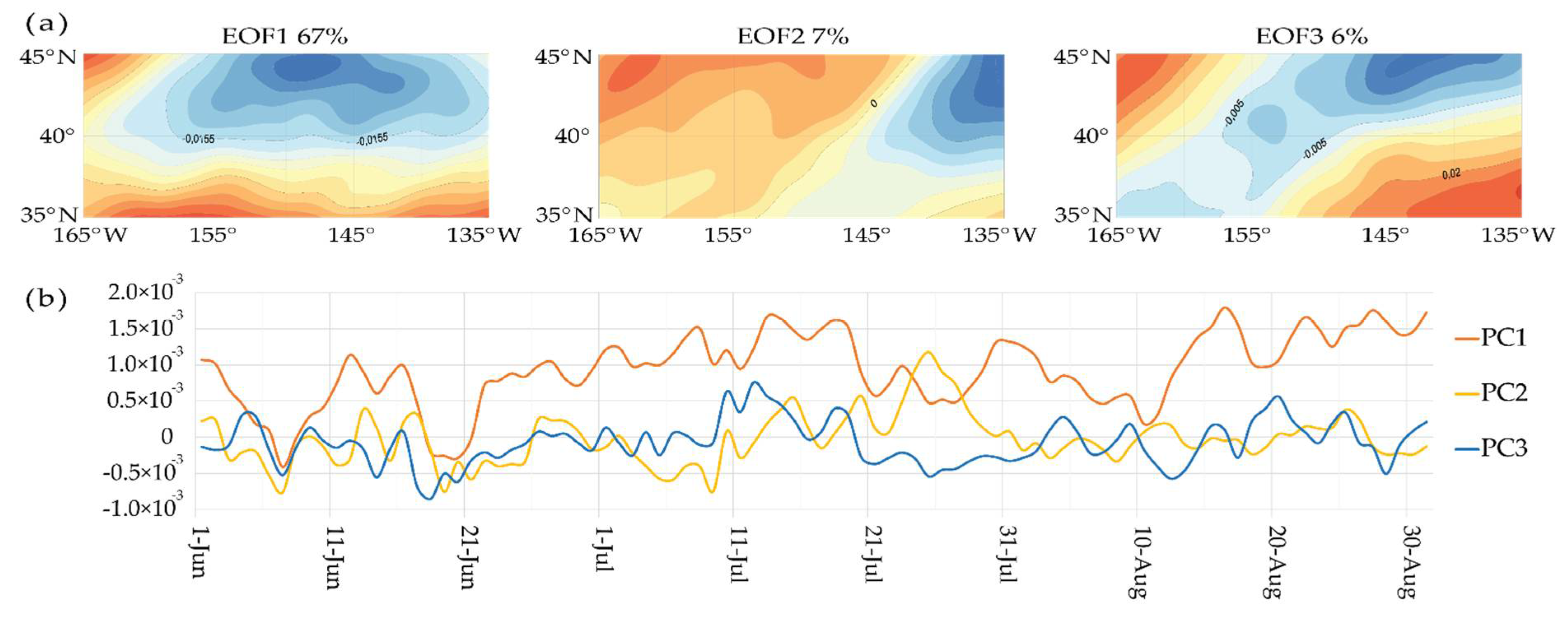
3.1. Spatial Structure of the Hawaiian Anticyclone Vorticity

A decomposition into empirical orthogonal functions of the vorticity field at the level of 925 hPa was obtained to estimate the spatial structure of the Hawaiian High vorticity. The first three modes of the EOF expansion of the vorticity field is shown in Figure 1a. The first mode corresponds to the most typical position of the Hawaiian High, the second and third modes are a dipole and a tripole, respectively, and in both cases, the region of negative vorticity shifts to the northeast of the region.

The first EOF mode explains 67% of the total variability, due to the fact that the data contains sufficiently large time-average component. The second and third EOF modes account for a much smaller percentage of spatial variability, 7% and 6% respectively. Thus, a very significant part of the variability is explained only by the first mode of the EOF expansion. This satisfies the applicability conditions for the individual vortex budget method.

Figure 1b shows the time series of principal components (PCs) for the first three modes of the EOF decomposition. The first mode of the EOF dominates during the study period, which corresponds to a sufficiently stable position of the Hawaiian High in the region. The predominant positivity of PC1 is due to that the average component is not removed from the data. The absolute values of the PC2 and PC3 are much smaller, and only in certain periods does their role increase (for example, the second mode becomes dominant on 24–27 July). The insignificant role of the second and subsequent EOF modes allows us to consider only the first EOF mode when analyzing the vorticity budget equation.

3.2. Spatial Structure of the Hawaiian High Vorticity

The terms of the vorticity budget equation were calculated from the ERA5 re-analysis data and then projected onto the first mode of the EOF decomposition (Figure 2). The positive values of the vorticity change at the level of 925 hPa correspond to the intensification of the anticyclone.

The most significant terms influencing the vorticity variation in the Hawaiian High are air temperature advection in the layer from the surface up to 200 hPa, vertical motions and vorticity variation in the upper troposphere. The contribution of heat fluxes and radiation balance is less noticeable. The influence of the latent heat flux is the least significant, which is typical for anticyclonic conditions; therefore, its influence will not be considered further. To clarify the contribution of each of the terms to the vortex dynamics, correlation coefficients were calculated for each of the terms on the right side of the equation with a vorticity change on the left side of the equation (

Table 1. Correlation coefficient between terms on the right side of the vorticity budget equation and vorticity change in Hawaiian High.

dξ1/dt	AT	W	ET	ER
0.58	−0.02	−0.30	0.14	0.10

).

The highest values of the synchronous positive correlation of vorticity change at 925 hPa are observed with vorticity change in the upper troposphere (0.58), which indicates the direct impact on the vorticity dynamics in the Hawaiian High. The growth of negative vorticity above the anticyclone contributes to its strengthening in the lower layers of the troposphere. A small but significant negative correlation (−0.30) is noted for the term related to vertical motions. This corresponds to theoretical ideas about the effect of negative feedback: ascending movements should strengthen the anticyclone and descending movements should weaken it [9].

The linear correlation between the vorticity change in the Hawaiian anticyclone and other factors on the right side of the vorticity equation is insignificant. Thus, the dynamics of the Hawaiian High is formed mainly by two factors: changes in the vorticity in the upper troposphere (200 hPa) and vertical motions.

4. Discussion

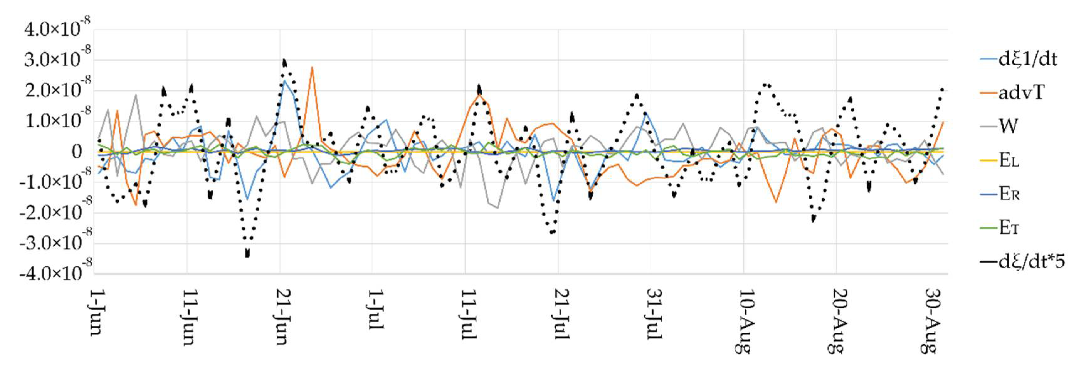
4.1. The Equation for the Coefficient y₁ (t) at the First Mode of the EOF Decomposition

Since the main part of the vorticity variability falls on the first mode of the EOF decomposition, our goal will be to obtain an equation for the coefficient $y_1\left(t\right)$. To do this, we will select in the depending on ${\xi }_2$ summands in the right side of Equation (2), the components containing only $y_1\left(t\right)$. In the expression with horizontal advection, we use the fact that the velocity $\overrightarrow{v}$ linearly depends on ${\xi }_2$, that is, $\overrightarrow{v}$ can be represented as the result of the action of some linear operator $\overrightarrow{V}\left[\right]$ on the function ${\xi }_2$:

$$\overrightarrow{v}=\overrightarrow{V}\left[{\xi }_2\right]=\overrightarrow{V}\left[{\displaystyle \sum _{i=1}^k{y}_i\left(t\right)\cdot V_i\left(\lambda ,\varphi \right)}\right]={\displaystyle \sum _{i=1}^k{y}_i\left(t\right)}\hspace{0.17em}\cdot \overrightarrow{V}\left[V_i\left(\lambda ,\varphi \right)\right]$$

(4)

where the multipliers $\hspace{0.17em}\overrightarrow{V}\left[V_i\left(\lambda ,\varphi \right)\right]$ depend only on coordinates, but do not depend on time, and can be found at a known wind velocity $\overrightarrow{v}$ using regression analysis. So, the equation for the coefficient $y_1\left(t\right)$ takes the form:

$$\frac{d{y}_1}{dt}=\frac{\partial {\xi }_1}{\partial t}\ast V_1+\frac{R}{f}\ln \frac{P_2}{P_1}{\nabla }^2\left\{y_1\left(\overrightarrow{V}\left[V_1\right],{\nabla }_h\right)\langle T\rangle +y_1{V}_1\sqrt{\frac{K_m}{2f}}\langle {\gamma }_a-\gamma \rangle -E_T+E_L+E_R\right\}\ast V_1+R_1$$

(5)

where the term $R_1\left(t\right)$ contains all the summands with the components of the EOF expansion of vorticity for all modes except the first one.

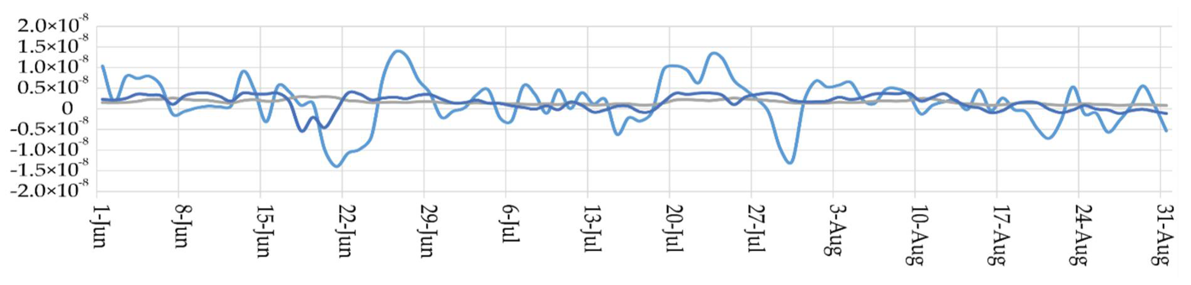
4.2. Estimation of the “Noise” Component in the Vorticity Budget Equation

Our approach suggests that the terms of the right side of the vorticity budget Equation (2) should lead to changes in vorticity in total. However, the exact equality of the left and right sides of the vorticity equation is not obtained. The presence of a discrepancy can be explained by the fact that we consider the equation only for the first mode of the EOF decomposition, which does not explain all the variability in the region. The other factor influencing the presence of a discrepancy is a number of assumptions made during the conversion of analytical to numerical equations. In addition, we did not take into account the ageostrophic part of the terms. So, an additional term $R\left(t\right)$ should appear on the right side of Equation (5), which includes both the component $R_1\left(t\right)$, and the discrepancy caused by phenomena whose scale is not taken into account in the re-analysis data, as well as all other unaccounted errors.

As the analysis shows, in addition to the noise component, the residual $R\left(t\right)$ contains non-random components. The technique proposed in [10,11,12] allows us to not completely discard the terms in the higher modes of the EOF decomposition, but to approximate them in terms of the lower modes and the noise term. It is also shown that if there was a quadratic nonlinearity in the original equation, when approximating the discarded components of the EOF decomposition, both quadratic and cubic terms with the explicit components arise. In our case, this means that the presence of quadratic terms with ${\xi }_2$ in the unaccounted factors (for example, the advection of vorticity) will lead to the appearance in $R\left(t\right)$ of terms proportional to the first, second and third degrees of $y_1\left(t\right)$. This means that $R\left(t\right)$ can be searched in the form:

$$R\left(t\right)={\alpha }_0+{\alpha }_1{y}_1\left(t\right)+{\alpha }_2{y}_1^2\left(t\right)+{\alpha }_3{y}_1^3\left(t\right)+\epsilon \left(t\right)$$

(6)

where ${\alpha }_0$, ${\alpha }_1$, ${\alpha }_2$, ${\alpha }_3$ are numerical coefficients and $\epsilon \left(t\right)$ is the noise term. The estimation of coefficients in (7) was carried out using regression analysis. Two hypotheses were tested: cubic and linear dependence of $R\left(t\right)$ on $y_1\left(t\right)$. The cubic expression from $y_1\left(t\right)$ better describes the behavior of the residual than the linear one (Figure 3). Analysis of the term $\epsilon \left(t\right)$ in the case of cubic approximation of the residual shows that it is Gaussian noise.

5. Conclusions

The temporal dynamics of the low-latitude circulation system (Hawaiian High) was analyzed using the vorticity budget equation. Atmospheric vortex quasi-permanently existing in a certain region was considered. Its evolution was determined by several factors: vorticity change in the upper troposphere, horizontal temperature advection, vertical motions, sensible and latent heat fluxes, and radiative balance. For the selected experimental period, the main part of the variability in the anticyclone was determined by the first mode of the EOF decomposition of the vorticity.

It was shown, that two factors make the greatest contribution to the evolution of anticyclonic vorticity in the considered case: the change in vorticity in the upper troposphere (feedforward) and vertical motions (feedback).

The right and left parts of the vorticity equation are not equal. The discrepancy is due to a number of factors related to re-analysis errors, the influence of the second and subsequent modes of the EOF expansion, and assumptions during the conversion from analytical to numerical equations. The maximum residual values correspond to the decay periods of the first mode of the EOF decomposition. The discrepancy consists of a non-random component and Gaussian noise, and the non-random component can be approximated by a cubic function of the time coefficient in the first mode of the EOF vorticity decomposition.

References

1. Palmen, E.; Newton, C. Atmospheric Circulation Systems: Their Structure and Physical Interpretation; Academic Press: New York, NY, USA; London, UK, 1969. [Google Scholar]
2. Zabusky, N.J.; Hughes, M.N.; Roberts, K.V.J. Contour dynamics for the Euler equations in two-dimensions J. Comp. Phys. 1979, 30, 96–106. [Google Scholar] [CrossRef]
3. Rudeva, I.; Gulev, S.K. Composite analysis of the North Atlantic extratropical cyclones in NCEP/NCAR reanalysis. Mon. Wea. Rew. 2011, 139, 1419–1446. [Google Scholar] [CrossRef]
4. Hannachi, A.; Jolliffe, I.T.; Stephenson, D.B. Empirical orthogonal functions and related techniques in atmospheric science: A review. Int. J. Climatol. 2007, 27, 1119–1152. [Google Scholar] [CrossRef]
5. Kislov, A.V.; Sokolikhina, N.N.; Semenov, E.K.; Tudrii, K.O. Analyzing the vortex as an integral formation: A case study for the blocking anticyclone of 2010. Russ. Meteorol. Hydrol. 2017, 42, 222–228. [Google Scholar] [CrossRef]
6. Kislov, A.V.; Sokolikhina, N.N.; Semenov, E.K.; Tudrii, K.O. Blocking Anticyclone in the Atlantic Sector of the Arctic as an Example of an Individual Atmospheric Vortex. Atmos. Clim. Sci. 2017, 7, 323–336. [Google Scholar] [CrossRef]
7. Petrosyants, M.A.; Semenov, E.K.; Gushchina, D.Y. Atmospheric Circulation in the Tropics: Climate and Variability; Maks Press: Moscow, Russian, 2005. (In Russian) [Google Scholar]
8. Hersbach, H.; Bell, B.; Berrisford, P.; Biavati, G.; Horányi, A.; Muñoz Sabater, J.; Nicolas, J.; Peubey, C.; Radu, R.; Rozum, I.; et al. ERA5 hourly data on pressure levels from 1979 to present. Copernicus Climate Change Service (C3S) Climate Data Store (CDS) 2018. [Google Scholar] [CrossRef]
9. Petterssen, S. Weather Analysis and Forecasting; McGraw-Hill: New York, NY, USA, 1956. [Google Scholar]
10. Majda, A.; Franzke, C.; Khouider, B. An applied mathematics perspective on stochastic modelling for climate. Philos. Transactions. Ser. A Math. Phys. Eng. Sci. 2008, 366, 2429–2455. [Google Scholar] [CrossRef] [PubMed]
11. Majda, A.; Franzke, C.; Crommelin, D. Normal forms for reduced stochastic climate models. Proc. Natl. Acad. Sci. USA 2009, 106, 3649–3653. [Google Scholar] [CrossRef] [PubMed]
12. Majda, A.; Timofeyev, I.; Vanden-Eijnden, E. A mathematical framework for stochastic climate models. Commun. Pure Appl. Math. 2001, 54, 891–974. [Google Scholar] [CrossRef]
Figure 1. (a) The spatial structure of the vorticity field at the level of 925 hPa, corresponding to the first three modes of the EOF analysis. (b) Principal components for the first three modes of the EOF decomposition.
Environsciproc 19 00004 g001
Figure 2. Time coefficients for the terms of the vorticity budget equation projected onto the first spatial mode of the EOF decomposition. The vorticity change values (black dashed line) are multiplied by a factor 5 for better representation.
Environsciproc 19 00004 g002
Figure 3. Approximation of the discrepancy of Equation (5) (light blue line) using linear (grey line) and cubic (dark blue line) expressions from y 1 ( t ) .
Environsciproc 19 00004 g003