Near-Reference Air Quality Sensors Can Support Local Planning: A Performance Assessment in Milan, Italy ^†

Abstract

At present, 4.2 million deaths occur every year due to ambient air pollution, according to the World Health Organization. In view of reducing such a figure, air quality monitoring and reliable data are essential. Nevertheless, local authorities in urban environments, where pollution levels are highest, often face a dilemma. On the one hand, the high costs of reference monitors make their large-scale adoption prohibitive, while the easily scalable low-cost sensors often feature significantly lower data quality and lack of calibration. Near reference monitors have been voiced as a promising solution, as they exhibit limited costs, though specific studies assessing their performance against reference monitors are still lacking. This article provides an in-depth assessment of three near reference sensors’ stations performance, through their collocation with regional reference monitors from December 2021 onwards. Two sensors were positioned at high-traffic locations, while the third recorded background pollution levels in Milan, Italy. The sensors’ performance was quantified not only via the coefficient of determination (R²) and the regression model, but also with the Mean Normalized Bias (MNB) and median values. After a first measurement period, sensors were re-calibrated to also appraise their behavioral change, generally exhibiting a performance increase. Results show high correlation for all hourly-recorded pollutants, with peaks for Ozone (O₃) (R² = 0.94) and BC (R² = 0.93). Although location-specific, such results show an interesting potential for near reference sensors in support of urban air quality planning.

1. Introduction

According to a recent estimate by the World Health Organization, 4.2 million premature deaths per year are caused by ambient air pollution in rural areas and cities worldwide [1]. With the aim of reducing this figure, reliable and accurate data measurements are needed, so to enable governmental institutions to enact evidence-based air quality policy measures.

Air quality monitoring institutions rely on reference monitors to assess air quality for regulatory purposes, which are characterized by high data quality standards, as required by the location-relevant air quality legislation [2]. Due to their data accuracy and precision, reference monitors are currently used to ascertain the regulatory compliance of air quality levels in urban areas. Nevertheless, such monitors involve significant investment costs, which often results in few installations spread over large urban areas as high costs make their large-scale adoption prohibitive. As an example, a European estimate for the purchase and installation of a multi-pollutant monitor in a purpose-built enclosure ranges from EUR 70 thousands to EUR 125 thousands [3], but global estimates suggest costs up to USD 180 thousands [2].

The current alternative to reference monitors has been low-cost sensors, which involve investment costs as low as EUR 25 and up to EUR 10 thousands [4]. Clearly, the lower investment cost of these monitors favors their large-scale deployment, although field tests show that low cost sensors’ data accuracy remains a challenge outside from laboratory conditions [5]. In addition, as shown by a review by Karagulian et al. [4], most low-cost sensors are “black boxes” that cannot be easily re-calibrated by users. Thus, considering the aging and drift to which these monitors are to be subjected, their data accuracy is expected to significantly decrease over time.

Near reference monitors have been recently voiced as a promising solution by industry actors, striking a balance between reference and low-cost monitors’ different costs and data quality [6]. Being mainly described by industry actors, this class of monitors includes instruments of intermediate costs between low-cost and reference monitors, but specific field assessments of their performance are still missing to date.

To overcome this gap, this article provides an in-depth performance assessment of three near reference sensors stations, belonging to the same instrument model in collocation with reference ones. Thus, the analysis aims at determining whether this kind of instrument can support air quality monitoring and planning in urban environments.

2. Materials and Methods

2.1. Tested Monitors’ Characteristics and Collocation’s Time Horizon

The performance of three identical multiparametric near reference sensor stations (Mod. MAS-AF300, Sapiens Environmental Technology Co., Ltd., Hongkong) was assessed through collocation with reference monitors of the institutional regional air quality network in Milan, Italy. The performance was assessed from mid December 2021 to June 2022. Two monitors were positioned at traffic sites (viale Marche and via Senato) while the third monitor was collocated with the urban background station (via Pascal).

Different emission source contexts were considered. One monitoring station (via Senato) was positioned within the so-called ‘Area C’ Congestion Charge Zone of Milan. The others remained outside of it, yet located within the so-called ‘Area B’ Low Emission Zone, covering a substantial part of the city’s territory. The monitoring stations’ geographical distribution and an example of collocation is shown in Figure S1.

The network of sensor stations was monitored via the supplier’s cloud data system. Sensor stations, producing real-time data, were periodically verified and, when needed, they were calibrated with ad-hoc supplier-proprietary digital procedure algorithms.

2.2. Performance Metrics

The sensors’ performance was quantified via the coefficient of determination (R²) and the regression model, i.e., the slope and y-intercept. In addition, the Mean Normalized Bias (MNB) and median values, which are often neglected in the literature [5], were calculated as defined in Equation (1).

$$MNB=\frac{\overline{y_i}-\overline{\widehat{y_i}}}{\overline{\widehat{y_i}}}$$

(1)

where $y_i$ is the near reference sensor’s measurement, $\widehat{y_i}$ is reference measurement, $\overline{y_i}$ is mean of $y_i$, $\overline{\widehat{y_i}}$ is mean of $\widehat{y_i}$.

In particular, the MNB quantified the average systematic distortion of the measurement process, i.e., the bias, in the near reference monitor with respect to the reference one.

2.3. Assessed Pollutants

In this article, examples of near reference sensors’ performances were assessed for four pollutants: nitrogen dioxide (NO₂); ozone (O₃); carbon monoxide (CO); and black carbon (BC). O₃ data are assessed only from mid-April, considering there are negligible levels of this pollutant during the winter season. NO₂ and CO were assessed both before and after an intermediate calibration.

3. Results and Discussion

3.1. Nitrogen Dioxide

The near reference sensor measuring NO₂ in the traffic site of viale Marche exhibits a high correlation (R² = 0.80) with the reference monitor at the beginning of the collocation (Figure 1a). This suggests that the linear regression model well suits the relationship between the near and the reference sensor in the winter period. After the intermediate calibration, the correlation between near and reference monitors improves, R² = 0.85, (Figure 1b) and median values difference remains rather low (

Table 1. Performance metric values for all pollutants included in the analysis.

Monitored Pollutant	Near Reference Median	Reference Median	MNB	Data Completeness	Sample Size
Ozone—via Pascal	74.55 μg/m3	73.30 μg/m3	0.05	95%	1457
Black carbon—via Pascal	1.90 μg/m3	1.30 μg/m3	0.47	96%	3752
Carbon monoxide—via Senato (pre-calibration)	1.35 mg/m3	1.10 mg/m3	0.18	99%	921
Carbon monoxide—via Senato (post-calibration)	0.66 mg/m3	0.70 mg/m3	−0.07	98%	2032
Nitrogen dioxide—viale Marche (pre-calibration)	50.71 μg/m3	52.20 μg/m3	−0.02	99%	2089
Nitrogen dioxide—viale Marche (post-calibration)	33.94 μg/m3	26.90 μg/m3	0.33	85%	814

). A reduced performance can be observed by looking at the slope and intercept, probably due to lower airborne concentration values in the spring period. In order to better interpret this phenomenon, an analysis distinguishing between day and night hours was performed. In this way, the sensor performance at lower concentrations was separated from that at higher concentrations. In fact, at night, lower NO₂ concentrations values are expected as a result of reduced traffic fluxes, mainly during spring period, when a lower frequency of typical Po Valley winter thermal inversions occurs.

As can be seen in Figure 1c,d, the lower (night) values feature a lower regression’s slope, both in winter (Figure 1c) and spring (Figure 1d). At the same time, it is noticeable that during the day, which is characterized by traffic, at higher concentration levels, the near reference sensors performance improves both in terms of coefficient of determination (R² = 0.87) and slope.

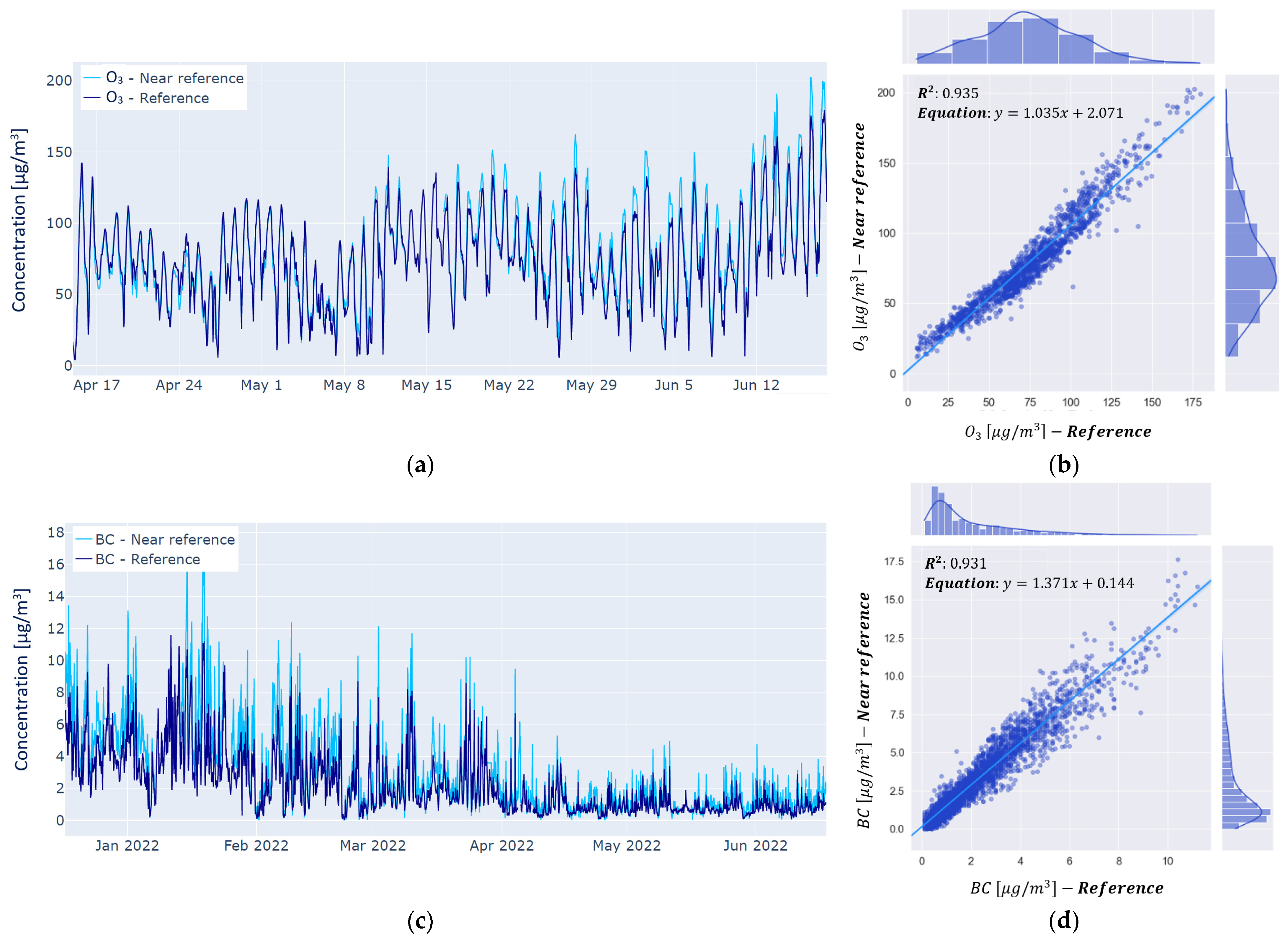
3.2. Ozone

The near reference sensor measuring O₃ in via Pascal exhibits a high correlation with the reference monitor (Figure 2a,b).

In particular, the sensor exhibits a high R², equal to 0.94, suggesting that the linear regression model well suits the relationship between the near reference sensor and the reference monitor. In addition, the slope of the linear regression model equals 1.04, while the y-intercept is 2.07 µg/m³. Thus, an overall linear and proportionally increasing relationship between the near reference sensors and reference monitor can be expected. A bias (MNB) of 0.05 was observed, indicating a low systematic deviation between the near reference sensor and reference monitor (Table 1).

3.3. Black Carbon

The near reference BC sensor in via Pascal shows a good correlation with the reference BC monitor in the same location (Figure 2c,d). Specifically, the instruments feature a very high R² value (0.93). As a result, the relationship between the near reference sensor and reference monitor can be well approximated by a linear regression model. In this case, a very small y-intercept (0.14 µg/m³) is accompanied with by a slope of 1.37.

The MNB, equal to 0.47, suggests a systematic difference between the near and reference monitor (Table 1), that can be attributed to the different measuring principle of the two instruments. For this pollutant, a periodic check of fluxes of the near reference monitor is performed. An optical calibration can be considered for improving performance.

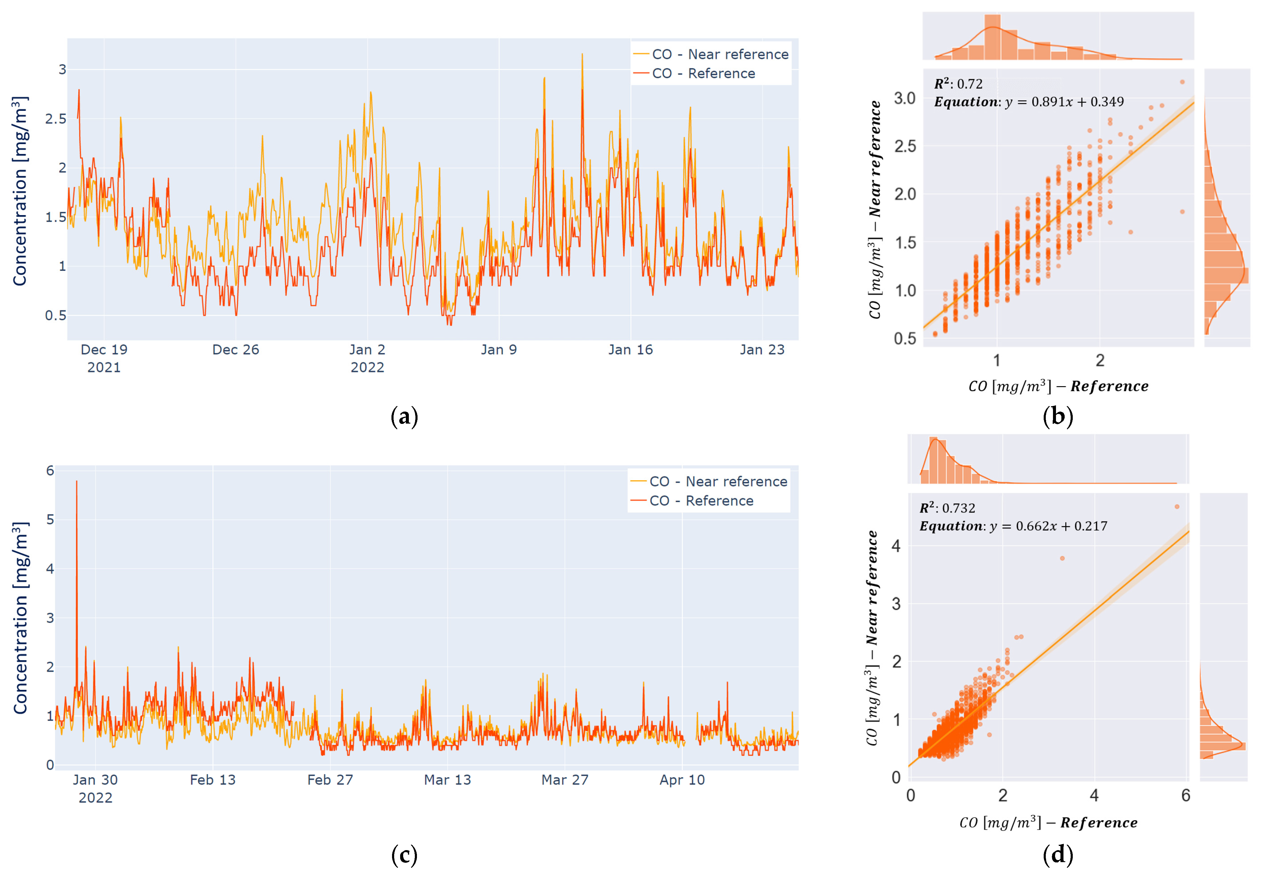
3.4. Carbon Monoxide

CO underwent a recalibration during the study period of the current analysis. For this reason, two sensor behaviors can be distinguished: before calibration (Figure 3a,b) and after (Figure 3c,d).

In particular, during the latter period, concentrations remained rather low and close to the lower detection limit of both reference and near reference sensors. The recalibration shows a positive effect on the R², the y-intercept of the linear regression model, as well as the MNB (Table 1). In fact, the R² slightly increases, and the y-intercept decreases to 0.22. In addition, the difference in medians also decreases, as does the bias, which sharply decreases to −0.07. Since this latter value indicates a difference between the mean concentration measured by the near reference sensor and the reference monitor, a negative value simply suggests a higher value for the reference monitor’s mean. Importantly, the significantly low MNB suggests no systematic deviation between the two monitors.

4. Conclusions

Near reference monitors have been voiced by industry actors as a good compromise between the cost and data quality of reference monitors and low-cost sensors. Additionally, they have been chosen by several city administrations to further enhance air pollution mapping and policy effectiveness.

In this article, the data quality of a sample of near reference monitors was assessed. Overall, very good correlations with reference monitors appear for all the pollutants analyzed (R² > 0.72). In particular, a very high correlation was found for O₃ (R² = 0.94) and BC (R² = 0.93).

Calibration operations prove to be important in obtaining better performance of sensors, although performance may not always simultaneously increase according to all performance metrics. Thus, multiple calibrations attempting to increase the performance along all these different dimensions should be considered.

In general, the present study suggests that the investigated multi-parameter compact stations can support urban authorities in air quality monitoring for policy implementation, following periodic calibrations and taking into consideration the on-field performances for the different pollutants.

References

- WHO. “Ambient (Outdoor) Air Pollution”. World Health Organization (WHO) Fact Sheets, 22 September 2021. Available online: https://www.who.int/news-room/fact-sheets/detail/ambient-(outdoor)-air-quality-and-health (accessed on 5 June 2022).
- Schäfer, K.; Lande, K.; Grimm, H.; Jenniskens, G.; Gijsbers, R.; Ziegler, V.; Hank, M.; Budde, M. High-Resolution Assessment of Air Quality in Urban Areas—A Business Model Perspective. Atmosphere 2021, 12, 595. [Google Scholar] [CrossRef]
- Mooney, D. Guide for Local Authorities Purchasing Air Quality Monitoring Equipment; AEA Technology Plc.: Harwell, UK, 2006; AEAT/ENV/R/2088 Issue 2. Available online: https://uk-air.defra.gov.uk/assets/documents/reports/cat06/0608141644-386_Purchasing_Guide_for_AQ_Monitoring_Equipment_Version2.pdf (accessed on 5 June 2022).
- Karagulian, F.; Gerboles, M.; Barbiere, M.; Kotsev, A.; Lagler, F.; Borowiak, A. Review of Sensors for Air Quality Monitoring; Publications Office: Luxembourg, 2019; Available online: https://data.europa.eu/doi/10.2760/568261 (accessed on 5 June 2022).
- Kang, Y.; Aye, L.; Ngo, T.D.; Zhou, J. Performance evaluation of low-cost air quality sensors: A review. Sci. Total Environ. 2021, 818, 151769. [Google Scholar] [CrossRef] [PubMed]
- Boehm, S. Recent Regulations from California to London—What Is the Impact on the Air Quality Monitoring Landscape? 2020. Available online: https://www.eventscribe.com/2020/ACEVIRTUAL/fsPopup.asp?efp=SlJUWEJSWkExMTIwMw&PresentationID=739104&rnd=0.8349781&mode=presinfo (accessed on 5 June 2022).