Abstract
Atmospheric/plume turbulence parametrization is an important input for the estimation of dispersion of pollutants from vehicular exhaust. A Three-Phase Turbulence (TPT) model was proposed by Madiraju and Kumar (2021) considering the critical parameters such as initial vertical plume spread, downwind distance, wind velocity, additional spread due to vehicular wake, thermal turbulence, atmospheric turbulence, road width, residence time and mixing height of mobile source dispersion. The flow regime of the TPT model is divided into the initial phase, transition phase, and dispersion phase. The paper presents the performance of these two types of modeling approaches based on the current practice using dispersion curves from point sources and the new TPT model. The statistical indicators (including mean, sigma, bias, NMSE, correlation coefficient, FA2, and FB) are used as a performance measure to identify the variations in the model results using observed data from three different field studies. The study indicates the changes in the performance of the basic mobile source model with the use of the TPT model. Overall, the performance of the basic mobile source dispersion model has improved slightly by using the TPT model.
1. Introduction
Dispersion and chemical transformation in the atmosphere using mathematical or numerical techniques is called air pollution dispersion modeling [1]. The dispersion modeling is based on the physics and chemistry involved in the process of advection/dispersion of contaminants and could predict and estimate the concentrations of contaminants by considering the origin of source, composition, emissions, traffic data, and meteorology [2]. Analytical/numerical techniques are used to simulate ground-level concentration in air quality models. Typical inputs of air quality modeling include source information, meteorological data, and the surrounding terrain [3].
The small-scale, irregular air motions characterized by winds that vary in speed and direction are called turbulence in the atmosphere [4]. Atmospheric turbulence is vital in causing the mixture and distribution of atmospheric gasses, water vapor, and other substances and hence it is an important parameter in air quality modeling [5]. Along with atmospheric turbulence, other critical parameters in air quality modeling are atmospheric stability, initial vertical plume spread, downwind distance, wind velocity, additional spread due to vehicular wake, thermal turbulence, road width, residence time, and mixing height of mobile source dispersion [6]. The improvement in the performance of mobile source models over the last 50 years is achieved by improving the theoretical basis of the dispersion equations and developing dispersion coefficients based on either theory or field experiments. Madiraju and Kumar (2021) proposed a new Three-Phase turbulence model to calculate the vertical spread of mobile source plume by combining the current concepts of atmospheric turbulence and plume spread observations based on field data. The purpose of this study is to simulate the ground level concentrations using a basic model without following the three-phase turbulence model (MODEL-A) and compare results with the same basic model using dispersion coefficients for point sources (called MODEL-B and with following the three-phase turbulence model). Statistical indicators are used to assess the performance of the basic model under these two cases.
2. Three Phase Turbulence Model (TPT)
A TPT model was developed by considering the critical parameters such as initial vertical plume spread, downwind distance, wind velocity, additional spread due to vehicular wake, thermal turbulence, atmospheric turbulence, road width, residence time, and mixing height of mobile source dispersion [7]. The mobile source plume is categorized into three phases: Initial, transition, and dispersion phases [8]. The flow regimes for the mobile sources are proposed based on the field studies conducted. Most of the existing models still consider the turbulence model from stationary sources. TPT is a newly proposed turbulence model that can be predominantly used for mobile source plume dispersion. Vertical dispersion coefficient () is one of the critical components that affect model predictions [9]. Initial vertical dispersion () has an impact on the plume dispersion. Consider a highway with mobile source vehicles. Consider wind orientation at an angle to the length of the road. The width of the road is W (m) and is the mean wind speed (m/s). In the TPT model the formulation used for [10] is
As discussed earlier the mobile source plume is categorized into three phases: Initial, transition, and dispersion phases (See Figure 1). The initial phase is near the mobile sources and the highway.
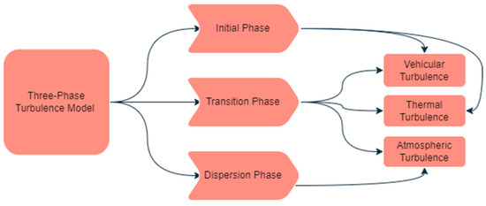
Figure 1.
The phases in the TPT model and associated turbulence.
2.1. Initial Phase
The Initial Phase is the first flow regime, which is near the mobile sources and the highway. The mobile source plume dispersion is dominated by vehicular and thermal turbulence in this phase. The average downwind distance up to which the initial phase is observed for the light-duty vehicles is 6.5 m from the highway. This is based on a study by Benson [11], the width of the mixing zone in the downwind direction was estimated by Benson as the width of the roadway and an additional 3 m. It is assumed that is constant up to 6.5 m, which is based on the summation of the width of the road 3.5 m and 3 m from the edge of the road. In the initial phase, the vertical dispersion is equal to the initial vertical dispersion.
2.2. Transition Phase
The Transition Phase is the second flow regime, a little far from the mobile source and the highway. The Transition Phase is in the wake area created by wind flow. The Transition Phase includes the effect of thermal turbulence, vehicular turbulence, and atmospheric turbulence. vehicular turbulence means the turbulence created by the motion of the vehicle. thermal turbulence is created by the heating of the ground due to solar radiation. atmospheric turbulence means irregular air motions characterized by winds. Based on the field turbulence parametrization of light-duty vehicles. The transition phase is considered from 6.5 m to 50 m of downwind distance from the source. The value of 50 m will depend on the type of vehicles on the highway and could be as high as 150 m for large trucks, as pointed out by Yu et al. [12,13].
2.3. Dispersion Phase
The Dispersion Phase is the third flow regime, away from the vehicular wake area. The mobile source plume dispersion in the dispersion phase is significantly dominated by atmospheric turbulence. Based on the filed turbulence parametrization of light-duty vehicles, the dispersion phase is considered from 50 m to the end of the plume [12,13].
3. Basic Model
A basic model to calculate the concentration of the pollutant from a mobile source is based on the convective–diffusion equation for a constant wind velocity and eddy diffusivity. The solution given in Equation (2) is taken from the textbook by Wark et al. [14]:
where H is the effective height of the plume from the vehicle, and q is the source strength per unit distance. The equation is divided by the sin where is the angle between the wind direction and the line source. (Note: is not used in the computation when the angle is less than 45 degrees) [14]. The horizontal component is neglected in Equation (2) since the crosswind diffusion is assumed to be self-compensating.
4. Performance Evaluation
The performance of the basic model is assessed initially by simulating the ground level concentrations of the air pollutants with multiple data sets without and with implementing the TPT model. The performance measures (discussed in Section 4.3) are then computed by running through a model evaluation software (BOOT in this study). BOOT results are compared to identify the performance change after implementing the TPT model.
4.1. Data
Three data sets are considered in the evaluation of the simple dispersion model. They are CALTRANS, Idaho Falls, and Raleigh data sets. The descriptive statistics of these MODEL-A and MODEL-B data sets are discussed in Table 1.

Table 1.
Descriptive statistics of the data sets used in this study.
- (a)
- Data 1: The CALTRANS highway 99 Tracer experiment was conducted in the 1980s in California near Highway 99 to measure SF6 (Sulfur hexafluoride). Approximately 35,000 vehicles were observed in traffic daily [15]. The concentrations of SF6 are measured at 0 m, 32.14 m, 64.28 m, and 128.56 m downwind distance in the North and South directions. The wind speed ranges are observed to be 0.2 m/s–6 m/s [16].
- (b)
- Data 2: Idaho Falls Tracer experiment was conducted to measure SF6 in 2008 at Idaho Falls, a city in Idaho. The SF6 is measured in this field experiment for 18 m, 36 m, 48 m, 66 m, 90 m, 120 m, and 180 m downwind distances. The source is modeled with a unit emission rate because the measured emission rates are slightly different for each day. The emission rates for day 1, 2, 3, and 5 are 0.05 g/s, 0.04 g/s, 0.03 g/s, and 0.03 g/s respectively [17].
- (c)
- Data 3: Raleigh 2006 experiment was conducted to measure NO (Nitric oxide) in Raleigh, North Carolina. Approximately traffic observation was 125,000 vehicles/day [18]. The emission factor used is 0.5 g/vehicle/km. NO is measured at 21.16 m and 30.36 m downwind distances [19].
4.2. Evaluation Tool
BOOT has been primarily used to evaluate the performance of air dispersion models. It provides concise information on model performance. The current study uses Version 2.0 of the BOOT software (Joseph C. Chang and Steven R. Hanna, Fairfax, VA, USA). This software is significant in providing the summary of confidence limit analyses based on percentile confidence limits. It also provides a summary of performance measures for the considered dispersion models [20].
4.3. Performance Measures
It is necessary to consider multiple performance measures, as each measure has advantages and disadvantages and there is not a single measure that is universally applicable to all conditions. The relative advantages of each performance measure are partly determined by the distribution of the variable of interest. Linear measures of FB (Fractional Bias) and NMSE (Normalized Mean Square Error) are strongly influenced by infrequently occurring high observed and predicted concentrations. The fraction of predictions within a factor of two of observations (FA2), on the other hand, is the most robust measure, because it is not overly influenced by high and low outliers. Along with FB, NMSE, and FA2; the correlation coefficient (r) is also an important performance measure used in this study. The ideal values and suggested ranges of performance measures for a better-performing model are presented in Table 2. FBFN can be considered as the underpredicting (false-negative) component of FB. Similarly, FBFP can be considered as the overpredicting (false-positive) component of FB, i.e., only those (Co- Observed concentration in the field, Cp-Predicted concentration using a mathematical model) pairs with Cp > Co are considered in the calculation. All these performance measures are simulated using BOOT software [7,20,21].
Table 2.
Significant performance measures were used in this study with their ideal values and suggested ranges for a better-performing model.
4.4. Results
The ground-level concentrations (that are simulated using the basic model) are run through the BOOT software. The BOOT software output results generated for the three data sets for stable and unstable atmospheric conditions are listed in Table 3. In the BOOT analysis, it was considered that MODEL-A is the basic model without following the TPT model and MODEL-B is also the same basic model following the TPT model.
Table 3.
BOOT output results for the simple model for the three considered data sets at stable and unstable atmospheric conditions.
In the BOOT output file ‘N’ represents the number of data points considered in each data set. Each block represents each data set considered to run the BOOT software.
Since the basic model used in this study is a widely used model by many researchers and students, all the performance measures (statistical indicators) computed are in the satisfactory range suggested in the literature. In the nominal (median) results, the mean and standard deviation values of MODEL-A are significantly close enough when compared with observed values. But the MODEL-B results show that the mean and standard deviation values of the basic model have improved. The nominal results also indicate that all the other statistical indicators also improved slightly.
The mean values of the model predicted concentrations for Data set 1 stable, Data set 2 stables of MODEL-A are close to the observed values. Data set 2 is unstable Data set 3 is stable, and the unstable of MODEL-B is close to observed values. The sigma values of the model predicted concentrations for Data set 1 and data set 3 stables of MODEL-A are close to the observed values and MODEL-B sigma values are close to observed values in all the other data sets.
The Bias values of MODEL-A and MODEL-B are higher than the ranges of a better-performing model. But the values of MODEL-B are slightly improved than MODEL-A. The Bias value for a perfect model is 0, which is practically impossible [26].
NMSE emphasizes the scatter in the complete dataset. NMSE reflects both systematic and unsystematic (random) errors in the concentrations. The ideal value of a perfect model will be 0 [27]. However, the results indicate that MODEL-A and MODEL-B have better NMSE values. The best NMSE value observed for MODEL-A for data set 2 (both stability conditions) and data set 3 (unstable condition) is 0.11. The best NMSE value is observed for MODEL-B for data set 2 (unstable condition) and data set 3 (unstable condition) is 0.11.
The correlation coefficient gives an indication of the linear relationship between the predicted and observed values. A perfect model has a correlation coefficient value of 1 [28]. Model-A and MODEL-B have correlation coefficients ranging from 0.58 to 0.74 and 0.67 to 0.8 in all three data sets. This indicates that MODEL-B predicted concentrations are more significantly correlated than MODEL-A.
The FA2 is defined as the percentage of predictions within a factor of two of the observed values. The ideal value for the factor of two is 1 (100%) [29]. The fraction of predictions within a factor of two observations. The air quality model with more than 0.8 value of FA2 is called a better performing model. The highest values of FA2 for MODEL-A and MODEL-B are observed as 0.81 and 0.88 respectively for data set 1 for unstable atmospheric conditions.
The FB values for both the models are less than 0.5 and close to 0, which means both MODEL-A and MODEL-B are better performing. However, it can be observed that all the FB values are negative, which means that most of the model predictions are less than the observed values (under-predicting). If the point of (FBFN, FBFP) = (2, 0) means that predictions are zero everywhere, but all observations are finite. If the point of (FBFN, FBFP) = (0, 2) means that observations are zero everywhere, but all predictions are finite. Since both FBFN and FBFP have values greater than 0 and less than 2 which means all the observations and predictions are finite. If FBFN = FBFP = 0; then a model can be called as a perfect model [20,26].
5. Conclusions
Overall, the TPT model was implemented in a basic mobile source dispersion model, and the performance was assessed. Three data sets were used to assess and simulate the model’s predicted concentrations and compare them with the observed data. BOOT software is used to generate the comparison results. A comparison of results for the basic model with and without following the TPT model is given in Table 3 using the three data sets for stable and unstable atmospheric conditions. Various performance measures include meaning, sigma, bias, NMSE, correlation coefficient, FA2, and FB. The results indicate that there is a slight improvement in the model performance of the basic model after following the TPT model. Improvement in FB, NMSE, FA2 and r values are visible. The nominal results also show that the mean and standard deviation values of the simulations computed using MODEL-B are better than MODEL-A. Finally, these results indicate that following a separate turbulence model for the mobile source could improve model predictions. Note that the P-G dispersion coefficients used in the simple model were developed based on the work of Pasquill over 70 years ago and it is suggested that these dispersion coefficients should be replaced with the proposed turbulence parameterization in the TPT model.
Author Contributions
Conceptualization, A.K., S.V.H.M.; Investigation, A.K., S.V.H.M.; Method-ology, A.K., S.V.H.M.; Project administration, A.K.; Supervision, A.K.; Validation, A.K.; Writing—Original draft, S.V.H.M.; Writing—Review & editing, A.K. All authors have read and agreed to the published version of the manuscript.
Funding
This research received no external funding.
Institutional Review Board Statement
Not applicable.
Informed Consent Statement
Not applicable.
Data Availability Statement
The data (CALTRANS, Raleigh, and Idaho Falls), used in the study were taken from the CMAS (Community Modeling and Analysis System). Link: https://www.cmascenter.org/r-line/. Any other data are available from the authors.
Acknowledgments
The authors would like to thank The University of Toledo for providing the facilities to conduct the study.
Conflicts of Interest
The authors declare no conflict of interest.
References
- US EPA, Air Quality Dispersion Modeling—Screening Models. Available online: https://www.epa.gov/scram/air-quality-dispersion-modeling-screening-models (accessed on 15 June 2022).
- Leelőssy, Á.; Molnár, F.; Izsák, F.; Havasi, Á.; Lagzi, I.; Mészáros, R. Dispersion Modeling of Air Pollutants in the Atmosphere: A Review. Open Geosci. 2014, 6, 257–278. [Google Scholar] [CrossRef]
- Sharma, N.; Chaudhry, K.; Rao, C. Air Pollution Dispersion Studies through Environmental Wind Tunnel (EWT) Investigations: A Review. J. Sci. Ind. Res. 2005, 64, 549–559. [Google Scholar]
- Encyclopedia of Physical Science and Technology | ScienceDirect. Available online: https://www.sciencedirect.com/referencework/9780122274107/encyclopedia-of-physical-science-and-technology (accessed on 15 June 2022).
- Nieuwstadt, F.T.; Van Dop, H. Atmospheric Turbulence and Air Pollution Modelling: A Course Held in The Hague, 21–25 September, 1981; Springer Science & Business Media: Berlin/Heidelberg, Germany, 2012; Volume 1, ISBN 94-010-9112-9. [Google Scholar]
- Gifford, F. Atmospheric Dispersion Models for Environmental Pollution Applications. In Lectures on Air Pollution and Environmental Impact Analyses; American Meteorological Society: Boston, MA, USA, 1982; pp. 35–58. [Google Scholar]
- Madiraju, S.V.H.; Kumar, A. Development and Evaluation of SLINE 1.0, a Line Source Dispersion Model for Gaseous Pollutants by Incorporating Wind Shear Near the Ground under Stable and Unstable Atmospheric Conditions. Atmosphere 2021, 12, 618. [Google Scholar] [CrossRef]
- Madiraju, S.V.H.; Kumar, A. Examination of the Performance of a Three-Phase Atmospheric Turbulence Model for Line-Source Dispersion Modeling Using Multiple Air Quality Datasets. J 2022, 5, 198–213. [Google Scholar] [CrossRef]
- Mo, Z.; Liu, C.-H. Wind Tunnel Measurements of Pollutant Plume Dispersion over Hypothetical Urban Areas. Build. Environ. 2018, 132, 357–366. [Google Scholar] [CrossRef]
- Chock, D.P. A Simple Line-Source Model for Dispersion near Roadways. Atmos. Environ. (1967) 1978, 12, 823–829. [Google Scholar] [CrossRef]
- Benson, P.E. Modifications to the Gaussian Vertical Dispersion Parameter, Σz, near Roadways. Atmos. Environ. (1967) 1982, 16, 1399–1405. [Google Scholar] [CrossRef]
- Yu, Y.T.; Xiang, S.; Noll, K.E. Evaluation of the Relationship between Momentum Wakes behind Moving Vehicles and Dispersion of Vehicle Emissions Using Near-Roadway Measurements. Environ. Sci. Technol. 2020, 54, 10483–10492. [Google Scholar] [CrossRef] [PubMed]
- Yu, Y.-T. Parameterization of Vertical Dispersion Coefficient (σ z) near Roadway: Vehicle Wake, Density and Types. Ph.D. Thesis, Illinois Institute of Technology, Chicago, IL, USA, 2020. [Google Scholar]
- Wark, K.; Warner, C.F. Air Pollution: Its Origin and Control; Addison-Wesley: New York, NY, USA, 1981; ISBN 0-673-99416-3. [Google Scholar]
- Heist, D.; Isakov, V.; Perry, S.; Snyder, M.; Venkatram, A.; Hood, C.; Stocker, J.; Carruthers, D.; Arunachalam, S.; Owen, R.C. Estimating Near-Road Pollutant Dispersion: A Model Inter-Comparison. Transp. Res. Part D Transp. Environ. 2013, 25, 93–105. [Google Scholar] [CrossRef]
- Benson, P.E. Caline 4-A Dispersion Model for Predictiong Air Pollutant Concentrations Near Roadways; Federal Highway Administration Report FHWA/CA/TL-84/15; NTIS PB 85 211498/AS; California State Department of Transportation: Sacramento, CA, USA, 1984.
- Finn, D.; Clawson, K.L.; Carter, R.G.; Rich, J.D.; Eckman, R.M.; Perry, S.G.; Isakov, V.; Heist, D.K. Tracer Studies to Characterize the Effects of Roadside Noise Barriers on Near-Road Pollutant Dispersion under Varying Atmospheric Stability Conditions. Atmos. Environ. 2010, 44, 204–214. [Google Scholar] [CrossRef]
- Baldauf, R.; Thoma, E.; Hays, M.; Shores, R.; Kinsey, J.; Gullett, B.; Kimbrough, S.; Isakov, V.; Long, T.; Snow, R.; et al. Traffic and Meteorological Impacts on Near-Road Air Quality: Summary of Methods and Trends from the Raleigh Near-Road Study. J. Air Waste Manag. Assoc. 2008, 58, 865–878. [Google Scholar] [CrossRef] [PubMed]
- Venkatram, A.; Isakov, V.; Thoma, E.; Baldauf, R. Analysis of Air Quality Data near Roadways Using a Dispersion Model. Atmos. Environ. 2007, 41, 9481–9497. [Google Scholar] [CrossRef]
- Chang, J.C.; Hanna, S.R. Technical Descriptions and User’s Guide for the BOOT Statistical Model Evaluation Software Package, Version 2.0; George Mason University and Harvard School of Public Health: Fairfax, VA, USA, 2005. [Google Scholar]
- Rao, S.T.; Sistla, G.; Eskridge, R.E.; Petersen, W.B. Turbulent Diffusion behind Vehicles: Evaluation of ROADWAY Models. Atmos. Environ. (1967) 1986, 20, 1095–1103. [Google Scholar] [CrossRef]
- Riswadkar, R.M.; Kumar, A. Evaluation of the Industrial Source Complex Short-Term Model in a Large-Scale Multiple Source Region for Different Stability Classes. Environ. Monit. Assess. 1994, 33, 19–32. [Google Scholar] [CrossRef] [PubMed]
- Gudivaka, V.; Kumar, A. An Evaluation of Four Box Models for Instantaneous Dense-Gas Releases. J. Hazard. Mater. 1990, 25, 237–255. [Google Scholar] [CrossRef]
- Patel, V.C.; Kumar, A. Evaluation of Three Air Dispersion Models: ISCST2, ISCLT2, and SCREEN2 for Mercury Emissions in an Urban Area. Environ. Monit. Assess. 1998, 53, 259–277. [Google Scholar] [CrossRef]
- Kumar, A.; Bellam, N.K.; Sud, A. Performance of an Industrial Source Complex Model: Predicting Long-term Concentrations in an Urban Area. Environ. Prog. 1999, 18, 93–100. [Google Scholar] [CrossRef]
- Hedges, L.V.; Olkin, I. Statistical Methods for Meta-Analysis; Academic Press: Cambridge, MA, USA, 2014; ISBN 0-08-057065-8. [Google Scholar]
- Chang, J.C. Methodologies for Evaluating Performance and Assessing Uncertainty of Atmospheric Dispersion Models; George Mason University: Fairfax, VA, USA, 2003; ISBN 0-493-88223-5. [Google Scholar]
- Asuero, A.G.; Sayago, A.; González, A. The Correlation Coefficient: An Overview. Crit. Rev. Anal. Chem. 2006, 36, 41–59. [Google Scholar] [CrossRef]
- Bluett, J. A Comparison of Near Field Concentrations Predicted by AUSPLUME and CALPUFF. Clean Air Environ. Qual. 2000, 34, 27–32. [Google Scholar]
Publisher’s Note: MDPI stays neutral with regard to jurisdictional claims in published maps and institutional affiliations. |
© 2022 by the authors. Licensee MDPI, Basel, Switzerland. This article is an open access article distributed under the terms and conditions of the Creative Commons Attribution (CC BY) license (https://creativecommons.org/licenses/by/4.0/).