Network Science Tools Reveal System-Level Properties of SDG Interlinkage Networks ^†

Abstract

A growing literature constructs SDG interlinkage networks in order to understand the interplay between goals, co-benefits, and trade-offs present in Agenda 2030. Networks are constructed from a variety of sources including historical correlations, expert analysis, and literature surveys. However, beyond simply constructing such interlinkage matrices, it is important to explore their implications and to compute quantities that describe the system-level response of the network so that we can shed light on the overall network structure and its implications for policy decisions. In this paper, I review fundamental ideas of centrality and hierarchy that may prove useful in these system-level analyses, and I illustrate the ideas on two specific SDG interlinkage networks. Missing data is particularly problematic in such analyses, pointing to the ongoing need to improve data collection on the SDGs. In terms of the results for the specific SDG interlinkage networks that I consider, the network analyses reveal an asymmetry between the support for SDGs 1, 2, and 3 that the remaining goals provide, and a lack of influence in the other direction from SDGs 1, 2, and 3 to the other goals. These are much harder to observe in the absence of such system-level methodologies. In particular, the analyses highlight the possible lack of integration of SDGs 14 and 15, which may point to the need for additional policy interventions to support progress on these two goals in particular.

1. Introduction

Systems thinking provides a flexible bridge between quantitative and qualitative insights into complex phenomena. On the quantitative side, the last two decades have seen rapid growth in the analysis of complex networks and the development of new tools and methods that reach across scales to show how system-level outcomes result from local interactions.

Interlinkage networks for the Sustainable Development Goals [1] reflect the premise that progress on one SDG should influence (positively or negatively) progress on other goals [2]. For example, the seven-point scale proposed by Nilsson, Griggs and Visbeck [3] describes influences between goals in terms that include ‘reinforcing’ and ‘enabling’ for positive linkages, and ‘constraining’ or ‘counteracting’ for negative interlinkages. Behind this sits, implicitly or explicitly, a sense of the scope of likely, or perhaps merely possible, policy actions and the effects that a policy action aimed at one SDG might have on others, either for better (a ‘co-benefit’) or worse (a ‘trade-off’).

In network science terms, these indirect effects of policy actions form a network that is directed and weighted (allowing different interactions have different strengths). Moreover, unlike, for example, disease transmission networks, linkages can be negatively weighted, corresponding to trade-offs between goals rather than the co-benefits described by positive links. Such networks are typically constructed either from expert analysis, literature surveys, or by analysing correlations in timeseries for SDG indicators.

In this short paper, I explain and apply two sets of ideas from network science to interlinkage networks derived from goal-level interactions. The first, which I discuss in Section 2, is the idea of eigencentrality [4,5,6] which formally does not apply to complex networks with both positive and negative links, but, as has been shown previously, has an alternative and extremely useful interpretation, making it an important system-level statistic [7].

Section 3 discusses the second idea: the notion of hierarchy among the SDGs. Measures of overall hierarchy and directionality in complex networks have their roots in the computation and analysis of ecosystems, for example, food webs, but lend themselves also to the systemic analysis and quantification of prioritisation between the SDGs. Prioritisation of SDGs that lie further ‘upstream’ of others should enable those goals to be met while at the same time allowing benefits to flow through the network and, thus, allowing the whole system to benefit. In contrast, prioritisation of SDGs that lie far ‘downstream’ and, hence, have much lower levels of influence on other goals would not allow all SDGs to be met. I develop and discuss measures of hierarchy that help to identify points of leverage and maximum ‘downstream benefit’ to other goals in the network.

Section 4 presents results that test these ideas on a range of interlinkage networks using data from reports including the 2015 report published jointly by the ICSU and ISSC [8] and the Global Sustainable Development Report 2019 [9,10]. I present conclusions in Section 5.

2. Centrality Measures

Throughout the paper, we consider a network containing n nodes (and, in the case of the SDGs, usually n = 17) and a set of directed edges with either positive, negative, or zero weights given by the n-by-n adjacency matrix A. In the mathematical notation that follows our convention is that matrices are denoted by capital letters, not in bold, while vectors are denoted by lowercase bold letters. Elements of matrices and vectors are indicated by subscripts. The entry $A_{ij}$ is defined to be the weight of the edge from node j to node i, i.e., the influence of node j on node i. A common observation in network science is that some nodes appear to be more important or more ‘central’ to the network than others. The most fundamental notion of centrality is just to count the number of other nodes to which a node is connected. This gives rise to the centrality measures,

$$k_i^{in}≔{{\displaystyle \sum }}_{j=1}^n\left|A_{ij}\right| \mathrm{and}{k}_i^{out}≔{{\displaystyle \sum }}_{j=1}^n{\left|A_{ji}\right|}_{},$$

which are the (weighted) in-degree and out-degree of node i, respectively. The absolute value is required in order to avoid cancellation if a node has both positively and negatively weighted edges connected to it. Pham-Truffert et al. [11] referred to nodes that have a large in-degree as ‘buffers’ since they serve to combine the effects of many different nodes together, and to nodes that have a large out-degree as ‘multipliers’ as they serve to propagate the influence of a node to many other parts of the network. The total degree $k_i=k_i^{in}+k_i^{out}$ is a natural measure of the relative importance of node i in the network: this is the degree centrality of the node.

While simple, the concept of degree centrality can be criticised for its purely local nature; it counts the numbers of direct neighbours of a node but does not make any allowance for how connected those nodes themselves might be. A more robust measure of importance could, therefore, be obtained differently, through a slightly self-referential definition: the importance of a node is given by the weighted sum of the importance of the nodes to which it is connected. Mathematically, this implies that the importance $v_i$ of node i is given by

$$v_i=\frac{1}{\lambda }{\displaystyle \sum }_{j=1}^n{A}_{ij}{v}_j,$$

(1)

where $\lambda$ is a weighting parameter. This definition appears to be slightly circular since it demands knowing the importances $v_j$ of the nodes j to which node i is connected. One can imagine an iterative scheme, starting with estimated values for the $v_i$ and then recalculating them according to the formula until they converge. Such an approach works and gives the same answer in fact as the more mathematical approach which is to multiply up by the factor of $\lambda$ and to consider the equation $Av=\lambda v$, which is well known as the equation defining the eigenvectors $v$ and eigenvalues $\lambda$ of the matrix A. Generically, A has n distinct eigenvalues ${\lambda }_1\dots {\lambda }_n$ each with a corresponding eigenvector $v_1\dots v_n$. The eigenvalues are labelled in order, so that $Re({\lambda }_{1 })\ge Re\left({\lambda }_2\right)\ge \dots \ge Re\left({\lambda }_n\right),$ where Re denotes the operation of ‘taking the real part of’ for a possibly complex eigenvalue ${\lambda }_i$. For a matrix A that has non-negative entries, the largest eigenvalue ${\lambda }_1$ is guaranteed to be real and non-negative, and its corresponding eigenvector $v_1$ can be chosen so that it is non-negative as well; this is the Perron–Frobenius theorem. When the weighting parameter ${\lambda }_{}$ is fixed to be larger than ${\lambda }_1$ the iterations of Equation (1) converge to zero, which gives no information about centrality; reducing ${\lambda }_{}$ so that iterations of Equation (1) converge to a nonzero solution results in convergence to the (leading) eigenvector $v_1$ and, hence, to a meaningful answer. The elements of this ‘leading’ eigenvector are then a centrality measure which describes the relative importance of each of the nodes; this is known as eigenvector centrality, abbreviated sometimes to ‘eigencentrality’. For the SDGs, the meaning of eigencentrality can be intuitively related to the rate at which progress on other SDGs reinforces and drives progress on each SDG itself, as I now discuss in a slightly more general setting that copes with a larger class of interaction matrices that contain negative as well as positive interlinkages.

While the above is mathematically well defined only for non-negative matrices, it is often the case that a network with only a relatively small number of negative links will also have a leading eigenvector that has all entries non-negative; in such a case, it is tempting to continue to interpret the leading eigenvector as a centrality measure. But there is an additional context for interpreting the leading eigenvector: it is the dominant ‘response’ of the network when considered as a dynamic problem, evolving the state of the nodes over time. In the simplest possible case, consider the evolution equation

$$\frac{d{x}_i}{dt}={\displaystyle \sum }_{j=1}^n{A}_{ij}{x}_j,$$

(2)

where the rate of change of the state variable $x_i$ associated with node i depends linearly on the state variables at the nodes connected to i, mediated by the strength, direction, and sign of the interaction between the two nodes as captured by the interlinkage $A_{ij}$. The solution to Equation (2) is dominated, apart perhaps over a short initial transient phase, by the form of the leading eigenvector since it corresponds to the mode of maximum growth rate; the eigenvalues ${\lambda }_1\dots {\lambda }_n$ are the growth rates of these different modes of response, but $v_1$ dominates since (by definition) ${\lambda }_1$ is larger than all the others. In the interest of simplicity, I ignore the case where the two largest eigenvalues are real and equal, because this is generically unlikely to happen; moreover, it is observed not to be relevant to cases in practice such as the examples below, where the leading eigenvalue is clearly separated from the remaining n − 1 eigenvalues.

Hence, the leading eigenvector can be interpreted as the intrinsic mode of self-reinforcing growth of the state variables $x_1\dots x_n$ caused solely by their interactions. In the context of this work, and conscious of many caveats around the simplistic nature of Equation (2) and the coarse-grained representation this implies, $x_1\dots x_n$ can be viewed as the relative levels of progress made on each of the SDGs, interpreting the interlinkages as these reinforcing or balancing effects due to policy actions. This is aligned with the analysis of cross-impact matrices by several authors including notably Weitz et al. [2], who described their cross-impact matrix as attempting to address the question: “If progress is made on target x, how does this influence progress on target y?” In summary, large positive values of eigencentrality for an SDG indicate that progress on this SDG is well supported by progress on others, whereas smaller or negative values show that progress on this SDG is not an inevitable outcome of progress elsewhere and, hence, may deserve specific policy interventions.

3. Hierarchy in Directed Networks

Building interlinkage matrices with directed edges between nodes, rather than undirected ones (which would be interpreted as either mutually beneficial or mutually antagonistic relationships only), immediately leads to questions at the system level as to whether the network taken as a whole has a sense of directionality to it. The answer may be that it does not, for example, as would be the case of a network consisting of a cyclic ring of directed edges: all nodes have the same ‘level’ in the network. Contrastingly, a chain of positive directed edges all pointing in the same direction confers a clear hierarchy since, in our SDG context, progress on SDGs corresponding to nodes earlier in the chain results in co-benefits shared with SDGs further along the chain, but the reverse is not true.

In the context of the SDGs, it is clear that, while progress on goals related to societal change such as SDG 5 (gender equality) and SDG 10 (reduced inequalities) are highly likely to lead to progress on ‘human development’ goals such as SDG 1 (no poverty) and SDG 3 (good health and wellbeing), it is not so clear that all policy actions taken to reduce poverty or to improve healthcare would necessarily have co-benefits that included progress on SDG 5 or SDG 10; the progress on SDG 1 or SDG 3 could be a result of policy that failed to address persistent inequalities in gender or other population characteristics. So, how could we decide whether a given interlinkage network implies the existence of a hierarchy, and, if it does, how can we find which of the SDGs comes further up and which is lower down in the hierarchy that the directed network implicitly generates?

Following MacKay, Johnson, and Sansom [12], we can attempt to understand the extent to which a network has a hierarchy by assigning a level $h_i$ to each node i, and looking to minimise a function F of the levels that measures the overall amount of directionality in the network. MacKay, Johnson, and Sansom referred to this quantity as the ‘trophic confusion’ in the network, motivated by food webs where the structure of the trophic network is a key quantity of interest in order to understand an ecosystem. A generalisation of their initial idea is to include a collection of prespecified quantities $g_{ij}$, not necessarily related to the adjacency matrix entries, which provide a set of target spacings between the levels $h_i$. The values of the levels $h_i$ that minimise F can be determined by minimising the function

$$F\left(h\right)=\frac{{{\displaystyle \sum }}_{ij}{\left|A_{ij}\right|}_{}{\left(h_i-h_j-g_{ij}\right)}^2}{{{\displaystyle \sum }}_{ij}{\left|A_{ij}\right|}_{}}.$$

(3)

The form of F(h) in Equation (3) guarantees that it is non-negative and has minimum value zero when the spacings between levels satisfy exactly the requirements given by the $g_{ij}$. The denominator provides a normalisation of the values of F, enabling comparisons between different networks if the distribution of edge weights is the same; otherwise, it does not affect the values of h that minimise F. Equivalently, the levels $h_i$ that minimise F are given by solving the equation

$$\mathsf{\Lambda }h=vecdiag \left(A{G}^T-A^{T}G\right),$$

(4)

where the matrix $\mathsf{\Lambda }:=diag\left(k\right)-A^T-A$, the operation vecdiag() extracts just the elements of the main diagonal of the matrix and forms these into a column vector, $k$ is the vector of total degrees as defined previously above, G is the matrix whose entries are the target spacings $g_{ij}$, and the notation diag() forms a square matrix with the elements of the vector as the main diagonal of the matrix, with zeros elsewhere. In the case $g_{ij}=1$ for all i and j, the right-hand side $vecdiag \left(A{G}^T-A^{T}G\right)$ reduces to the difference between the (weighted) in-degree and out-degree.

Despite this rather detailed set of definitions, minimising the ‘trophic confusion’ quantity F is straightforward to implement computationally and provides a representation of a network that as far as possible provides an overall sense of directionality. This enables a visualisation of which nodes are furthest ‘upstream’ in the network and so influence most others, and which are furthest downstream and hence benefit most from co-benefits due to other SDGs.

4. Examples

To illustrate the concepts in the previous two sections, I analyse two interlinkage matrices for the SDGs at the goal level. The first of these was generated from an expert analysis [8] conducted by the International Science Council in 2015, when it was still the International Council for Science (ICSU), in partnership with the International Social Science Council (ISSC); I therefore refer to it as the ICSU Report. Although it is based on a qualitative analysis of policy interlinkages rather than historic data, this is one of the few reports to treat all the SDGs (except SDG 17 on partnerships for the goals) identically. Dawes (2020) [7] described in detail the methodology through which the expert opinions were turned into a quantitative cross-impact matrix. Essentially this involved interpretation of the direction of interlinkages from the report’s text, combined with an indication of the strength of an interlinkage given by the number of targets in the SDG that was being influenced that were mentioned as being impacted by progress on the influencing SDG.

The second interlinkage matrix considered is the one produced as part of the Global Sustainable Development Report (GSDR) 2019 [9,10,11]. This report carried out a literature survey of 177 global scientific assessments, UN flagship reports, and scientific articles on SDG interlinkages, wherever possible looking at the level of targets; here, their results are considered after aggregation to the goal level. A hand-coding of statements in these articles resulted in a set of 4976 separate positive and 782 negative interactions. Although there is considerable value in preserving the distinction between the positive and negative interactions separately, as discussed in more detail elsewhere [13], in this paper, for reasons of brevity, I discuss only the ‘net interlinkage’ matrix, adding positive and negative interlinkages together.

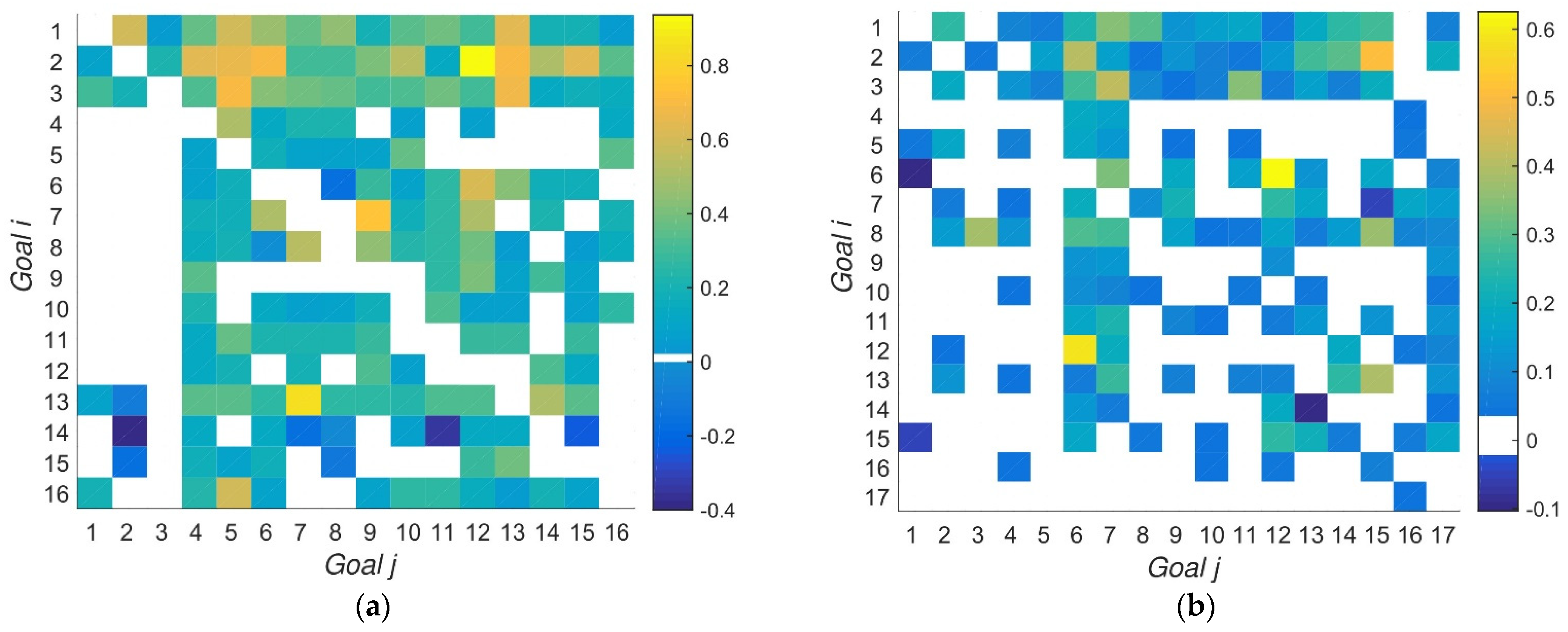
Figure 1 shows the interlinkage matrices derived from the ICSU and GSDR reports. Interlinkages are scaled to lie in the range [−1, 1], and those close to zero are replaced by whitespace to improve the readability of the figures. Diagonal entries are removed from the GSDR matrix to make this more directly comparable with the ICSU matrix; removing these entries turns out to have only a very minor effect [13]. In both cases, we observe that almost every SDG influences SDGs 1–3, as shown by the densely populated top three rows of each plot. But there are fewer influences from SDGs 1 to 3 on the remaining goals, as is shown by the relatively sparsely coloured first three columns on the left-hand side of each plot. This highlights a fundamental asymmetry in Agenda 2030: the first three SDGs are those on which most attention is focused, with SDGs 4 to 17 in some sense playing a subordinate role, supporting the fundamental development agenda and continuation from the Millennium Development Goals that SDGs 1–3 represent.

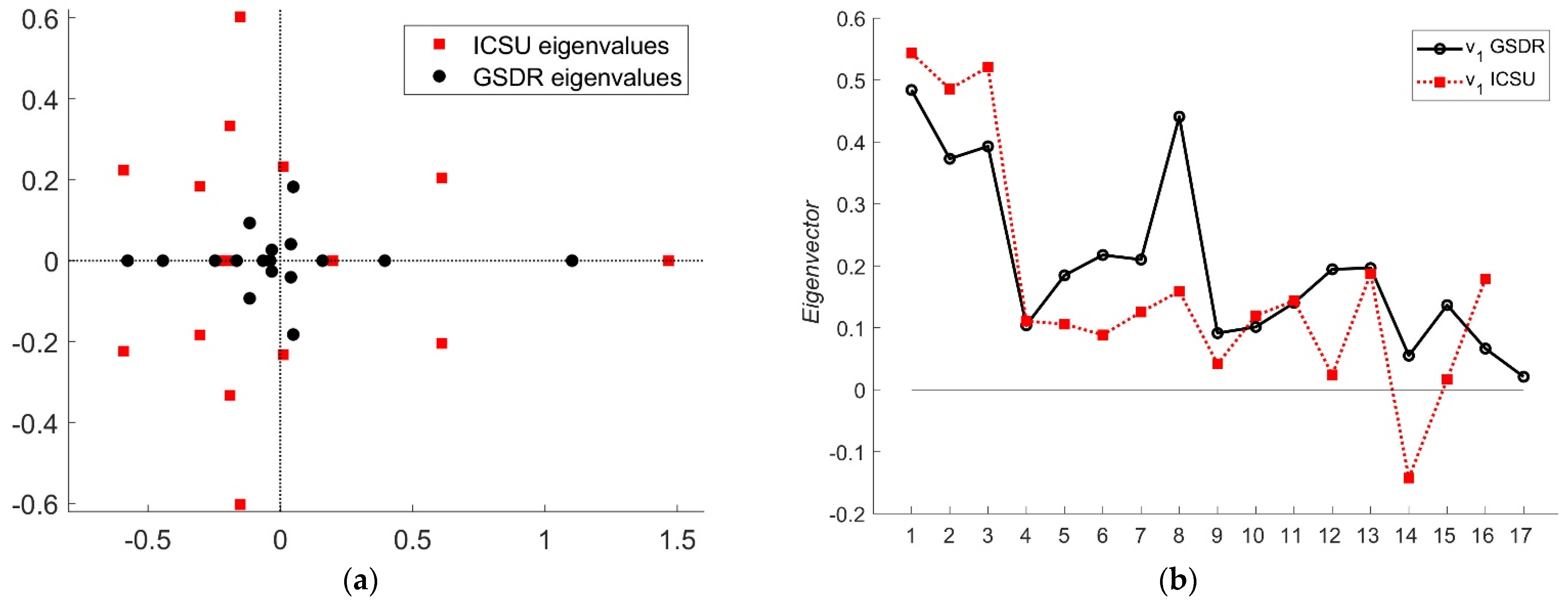
It is numerically straightforward to compute the eigenvalues and leading eigenvectors for the interlinkage matrices shown in Figure 1; the results are given in Figure 2. Figure 2a plots the eigenvalues in the complex plane. In both cases, there is a leading eigenvalue that appears far to the right of the remaining ones, leaving a significant gap between the leading eigenvalue and the next largest, for both the ICSU eigenvalues (red squares) and GSDR eigenvalues (black dots). This indicates that the domination of the behaviour of the networks by their leading eigenvectors is robust to perturbations of individual interlinkages. Detailed sensitivity analysis was carried out elsewhere [13]. The form of the leading eigenvectors themselves is shown in Figure 2b, again with GSDR eigenvectors in black and the ICSU ones in red. The lines joining the dots are just a guide to the eye; the data points show the components of the eigenvectors for each of the SDGs. The ICSU eigenvector has only 16 components since the ICSU analysis omitted SDG 17 completely.

The asymmetry noticed above is reflected in the high values of the eigenvector components for SDGs 1–3; these three SDGs are positively supported by many of the others, which would lead to greater progress on those goals, in the dynamical sense, and for them to be identified as among the most important in a centrality sense. The GSDR matrix has a particularly high component also for SDG 8 (decent work and economic growth), which is expected due to the relatively full row of interactions supporting SDG 8 in the interaction matrix in Figure 1b. The corresponding row for the ICSU matrix in Figure 1a also strongly supports SDG 8; however, in this case, the support is stronger for other SDGs and so SDG 8 does not emerge relatively better off.

Most concerning is the negative component of the leading eigenvector for SDG 14 (life below water) for the ICSU matrix. This suggests that the internal dynamics of the ICSU network would result in negative progress on SDG 14 when progress is made elsewhere. In terms of the interlinkage matrix, there are two strongly negative links, from SDG 2, and from SDG 11 to SDG 14; these are coloured dark blue in Figure 1a and point to significant trade-offs between the goals on zero hunger, sustainable cities, and progress on life below water.

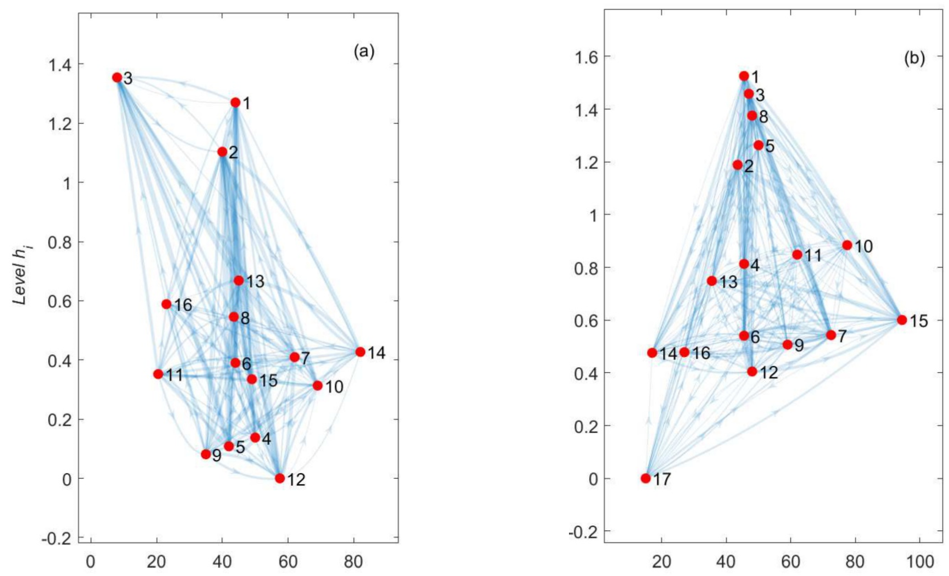
Finally, Figure 3 shows the results of minimising the trophic confusion measure F defined in Equation (3) for the two networks. In both parts of the figure, the relative levels of the SDGs are determined so that as many of the directed edges point upwards as possible. Hence, the influence between the SDGs generally runs from the bottom of each figure to the top. It can be seen that SDGs 1–3 consistently appear close to the top of the figures and SDG 12 appears low down. SDG 17 does not appear in Figure 3a since it was not included in the ICSU analysis. The relative horizontal positions of different SDGs have no meaning in terms of interlinkages; they are purely to make the figures as easy to interpret as possible. One surprise in Figure 3b is the relatively high position of SDG 5 (gender equality). This illustrates that the construction of these hierarchies depends on the robustness of the underlying data; as noted above, SDG 5 is rather sparsely represented in the literature review that the GSDR matrix was built from. One useful direction for future research would clearly be to develop measures of the robustness or sensitivity of these hierarchy calculations to missing or biased data.

5. Conclusions

The aim of this article is to introduce fundamental concepts in network science and show that they are able to contribute to the understanding of the study of SDG interlinkages, and in particular to the challenge of drawing system-level inferences from a set of individual pairwise interactions between the 17 SDGs, or indeed at the level of the 169 individual targets. After brief discussions of centrality in Section 1 and hierarchy in Section 2, two example networks were presented in order to illustrate the mathematical tools. The results illustrate the kind of overall conclusion that could be drawn about the structure of the interlinkage networks that was less obvious and certainly less quantifiable without the mathematical analysis available. The central conclusion is that progress on SDGs 1, 2, and 3 appears to be much more likely than progress on others, and that notably SDGs 14 and 15 are less well reinforced by the remainder of the goals, perhaps pointing to the need for additional policy interventions.

Of the many directions for future research, I touch on a couple of the most obvious and pressing. First, the degree to which the results are sensitive to biases, missing input data, and the details of the construction of any interlinkage network is obviously extremely important if the results are to have any validity. In part, detailed knowledge of the limitations, or indeed the rationale behind any one interlinkage network should be known and understood at the time of construction or data collection. The results for that network must then be interpreted in that light; without that context and background understanding, interpretation of the results is likely always to be misleading. In the context of the SDGs, the data gaps are well known but significant [13]. This report highlights both the gaps in coverage, noting for example that, for five of the SDGs, fewer than half of the 193 countries or areas have internationally comparable data, and also, more subtly, that the most recent data available in many cases is 5 or 6 years old. This lack of timeliness of data is noted as being particularly a concern for SDGs 1, 4, 5, and 13.

Given that the analysis of interlinkages through historic data depends on data being available for pairs of SDGs, so that their mutual dependency can be explored, the case for the involvement of expert analysis in the identification of interlinkages is perhaps made stronger, despite its more qualitative appearance and well-understood inherent subjectivity.

Recent work has explored mathematical measures of the sensitivity of the leading eigenvector and eigenvalue to perturbations in the network [14], and it is likely that similar approaches can be used to understand the robustness of the hierarchy calculations as well. The hierarchy calculations can also be formulated in many different ways, for example, making different choices for the target spacings $g_{ij}$ in Equation (3). There are indeed a number of different ‘natural’ choices for $g_{ij}$, and, more generally $g_{ij}$ allows the formulation of some kind of ‘prior structure’ that one might wish to impose on the answer, for example, pairs of SDGs whose levels should be more or less closely aligned than other pairs of SDGs due to some structural influence or geographical restriction. These issues deserve to be the subject of future investigations.

Other centrality measures, building on eigencentrality, might also be useful in order to explore more fully the connected nature of the network. There is related literature that allows the inclusion of three-way interactions between nodes in a directed network [15] (and references therein); this may be another helpful direction for these SDG networks in particular.

To conclude, while the construction of interlinkage networks is in itself a demanding and complex task, it appears to be gaining momentum as a way to visualise structure within the set of SDGs; it follows that appropriate network tools should be used to extract the system-level metrics and conclusions that follow from the interlinkage network. This second step, while of course inheriting biases present in the network data, is crucial in understanding in policy terms the emergent features that the interlinkage network represents and how best they should be addressed.