Abstract
Land-use changes adversely may impact ecological entities and humans by affecting the water cycle, environmental changes, and energy balance at global and regional scales. Like many megaregions in fast emerging countries, Tamil Nadu, one of the largest states and most urbanized (49%) and industrial hubs in India, has experienced extensive landuse and landcover change (LULC). However, the extent and level of landscape changes associated with vegetation health, surface permeability, and Land Surface Temperature (LST) has not yet been quantified. In this study, we employed Random Forest (RF) classification on Landsat imageries from 2000 and 2020. We also computed vegetation health, soil moisture, and LST metrics for two decades from Landsat imageries to delineate the impact of landscape changes in Tamil Nadu using Google Earth Engine (GEE). The level of vegetation health and drought for 2020 was more accurately assessed by combining the Temperature Condition Index (TCI) and Vegetation Condition Index (VCI). A Soil moisture index was subsequently used to identify surface permeability. A 75% expansion in urban areas of Tamil Nadu was detected mainly towards the suburban periphery of major cities between 2000 and 2020. We observed an overall increase in the coverage of urban areas (built-up), while a decrease for vegetated (cropland and forest) areas was observed in Tamil Nadu between 2000 and 2020. The Soil-Adjusted Vegetation Index (SAVI) values showed an extensive decline in surface permeability and the LST values showed an overall increase (from a maximum of 41 °C to 43 °C) of surface temperature in Tamil Nadu’s major cities with the highest upsurge for urban built-up areas between 2000 and 2020. Major cities built-up and non-vegetation areas in Tamil Nadu were depicted as potential drought hotspots. Our results deliver significant metrics for surface permeability, vegetation condition, surface temperature, and drought monitoring and urges the regional planning authorities to address the current status and social-ecological impact of landscape changes and to preserve ecosystem services.
1. Introduction
In the last three decades, the growth of landuse and landcover changes (LULC) have led to an enormous transformation in global landscape patterns [1,2,3,4]. Landscape changes result from many factors, including variability in abiotic conditions, such as climate, topography, and soils, biotic interactions that generate spatial patterning even under homogeneous environmental conditions and past and present patterns of human settlement. Land-use changes contributed to a reduction in vegetation health, surface permeability, and the occurrence of Surface Heat Island (SHI), Urban Heat Island (UHI), and drought [5,6,7,8]. It also drives climate change which affects humans and wildlife [9]. To enable sustainability and changes in the environmental structure, it is necessary to understand the subtleties of landcover change [10]. It is given high importance as most of the metropolitan cities have encountered substantial landcover changes over the decades [11,12,13]. Henceforth, these metropolitan areas consume more energy and produce severe environmental problems and thus lend land, water, and air pollution, which affects the functions of ecosystems [5,14,15]. Land Surface Temperature (LST) is an important parameter that influences the partition of energy between ground and vegetation and determines the surface air temperature [14]. LST is also an important factor in global climate change, vegetation growth, and UHI [15,16]. A sudden increase in land-use changes also affects environmental factors, such as rainfall, temperature, and groundwater level, which threatens the development process of the urban areas. Thus, examining the impact of landscape changes on vegetation and LST is crucial for efficient urban planning and management of land-use zones [17,18].
In India, one-third of the people live in cities [19]. During the last decade, the 4% increasing trend in urbanization expresses that people from the Tamil Nadu state and other neighboring states and millions of north Indian states people have relocated from rural areas to a metropolitan city to find a job and make their lives in cities [20]. The urbanization level in India went from 27.7% to 31.1%, with an increasing amount of 3.3% from 2001 to 2011 [21,22]. The statistics show that the urban population level in India will increase to 600 million, which doubles the rate from the present scenario by 2031 [23]. Due to urbanization, the cities in India are affected by unhygienic health conditions and damage to ecosystems [24]. In India, Tamil Nadu secured the first rank in urbanization among the fifteen primary states listed by the country [25]. The state has attained the uppermost level of urbanization with 43.86% in the country, based on the 2001 census [26]. Around 27 million people live in the metropolitan city of Tamil Nadu [27]. The urbanization pattern of Tamil Nadu is dispersed with municipalities in almost every district [28]. This rapid rise in urbanization in Tamil Nadu leads to many problems, including deforestation, water scarcity, flood, pollution, and other environmental damages [29]. Thus analyzing the impact of landscape changes on vegetation and land surface temperature over Tamil Nadu is crucial for sustainable urban planning and management [30].
Global Remote Sensing (RS) and satellite imageries processing techniques delivered considerable potential for landscape change patterns and vegetation change analysis. Thus, this study attempts to examine the impact of landscape changes on vegetation and land surface temperature using RS. Several studies have been carried out to examine the LULC changes, which are important indicators for examining the relationship between the environment and anthropogenic activities that can be attained from satellite images and other image processing techniques [31,32,33,34,35]. These are especially useful for a state like Tamil Nadu, where ground/field monitoring data are not available and scarce [32,36]. But the availability of satellite images helps to overcome this issue, especially Google Earth Engine (GEE) cloud computing platform provides efficient methods and freely available spatial data for storing, accessing, and analyzing spatial datasets on the high-performance servers [37]. GEE was launched by Google in 2010 and makes freely available RS datasets via its internet-based Application Programming Interface (API) provided by Python and a JavaScript web-based Interactive Development Environment (IDE) used to detect changes, landuse changes, map trends, landcover changes and quantify differences on the Earth’s surfaces and atmospheres [37].
The existing studies have focused mainly on the spatio-temporal relationship between LULC and environmental changes [10,32,38,39,40]. However, the multivariate relationship between LULC changes, vegetation, soil moisture, and land surface temperature has not been analyzed widely. This paper aims to fill this gap by examining the LULC changes effect on landuse vegetation and land surface temperature using GEE. The availability of GEE codes helps future research to integrate different datasets from Tamil Nadu at different resolutions.
The impact of land-use changes should be analyzed by considering the following research questions: (i) how could landscape changes make a variation in the Spatial and Temporal pattern of the land-use change? [41]; (ii) how could landscape changes affect the surface and land temperature conditions? [42], and (iii) how does the relationship exist between land-use change patterns and environmental factors (temperature, soil moisture, and vegetation) [43].
This paper is organized as follows: Section 2.1 and Section 2.2 describe the study area and data used in this work. Section 2.3 provides information about the observation and assessment of LULC Classification, Normalized Difference Vegetation Index (NDVI), Soil Adjusted Vegetation Index (SAVI), LST, Vegetation Condition Index (VCI), and Temperature Condition Index (TCI), respectively. Section 3 then combines the results from the individual stages of the research design to evaluate LULC changes to assess their impact on vegetation and LST. Finally, Section 4 and Section 5 provide the discussion and conclusion, respectively.
2. Materials and Methods
2.1. Study Area
Our study was undertaken in Tamil Nadu, a state located in the southern part of India [10], which has a seashore surrounded by one dimension and consists of various types of landscapes such as hilly terrain, wetlands, and forests [32]. It receives rainfall predominantly during the monsoon season in the western parts and interior districts, while the sea bordered districts receive rainfall from the emergence of cyclones [44]. Its capital city is Chennai and is surrounded on the north by Andhra Pradesh, on the east by the Bay of Bengal, on the west by Kerala, and on the south by the Indian Ocean (Figure 1). The Western Ghats and the Eastern Ghats mountain ranges converge in the Nilgiri hills in Tamil Nadu, making it the only state in India to have both. The total area of the state is 130,058 sq km making it the eleventh largest state in the country [45].
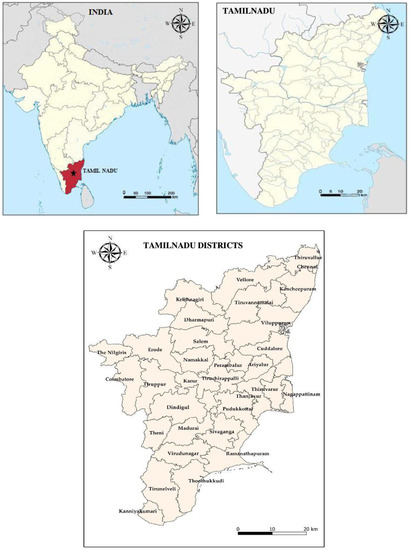
Figure 1.
Geographic location and area of Tamil Nadu State. The maps were generated using Google Maps.
The geographic location of Tamil Nadu spans between 11.12° N 78.65° E with an average elevation of 247 m and a maximum of 2599 m. Tamil Nadu has the largest tourism industry in India [29].
Tamil Nadu is the most urbanized state in India, one of the foremost industrialized states, and the highest tax-paying state to the central government. The urbanization trend of Tamil Nadu is supposed to exaggerate in the upcoming years. The climate of the region is sub-humid continental monsoon with an average annual temperature of 28.8 °C. The average yearly precipitation of the state is about 945 mm, of which 32% is through the southwest monsoon, and 48% is through the northeast monsoon. The cropping pattern in the majority of the states depends on the monsoon, if the onset of the monsoon is delayed or fails, then the probability of a drought event occurring is high [46].
2.2. Data
We used the Google Earth Engine (GEE) for most of the image processing and analysis for this paper. On the GEE computing platform, the static input variables are existing datasets, terrain, and geographic location, whereas the dynamic inputs are data acquired from RS [47]. Data were collected between October to December, which is usually the wet season because dry season data leads to low accuracy results on the vegetation and temperature changes while doing the mean of all images for every single year. So we only used the winter and monsoon data to classify landscape changes in vegetation along with the soil moisture over land surface temperature [46]. For the classification operation, data were collected from or uploaded to the GEE cloud computing platform. High-resolution satellite images from the Landsat sensor with a spatial resolution of 30 m and temporal resolution of 16-day images for the monsoon period October to December 2000, 2004, 2008, 2012, 2016, and 2020 were accessed from the GEE cloud computing platform. (Earth Engine Data Catalog: https://developers.google.com/earth-engine/datasets/catalog/, accessed on 1 January 2020) [48] (Table 1).

Table 1.
Technical description of the Landsat imageries used in this study.
2.3. Methods
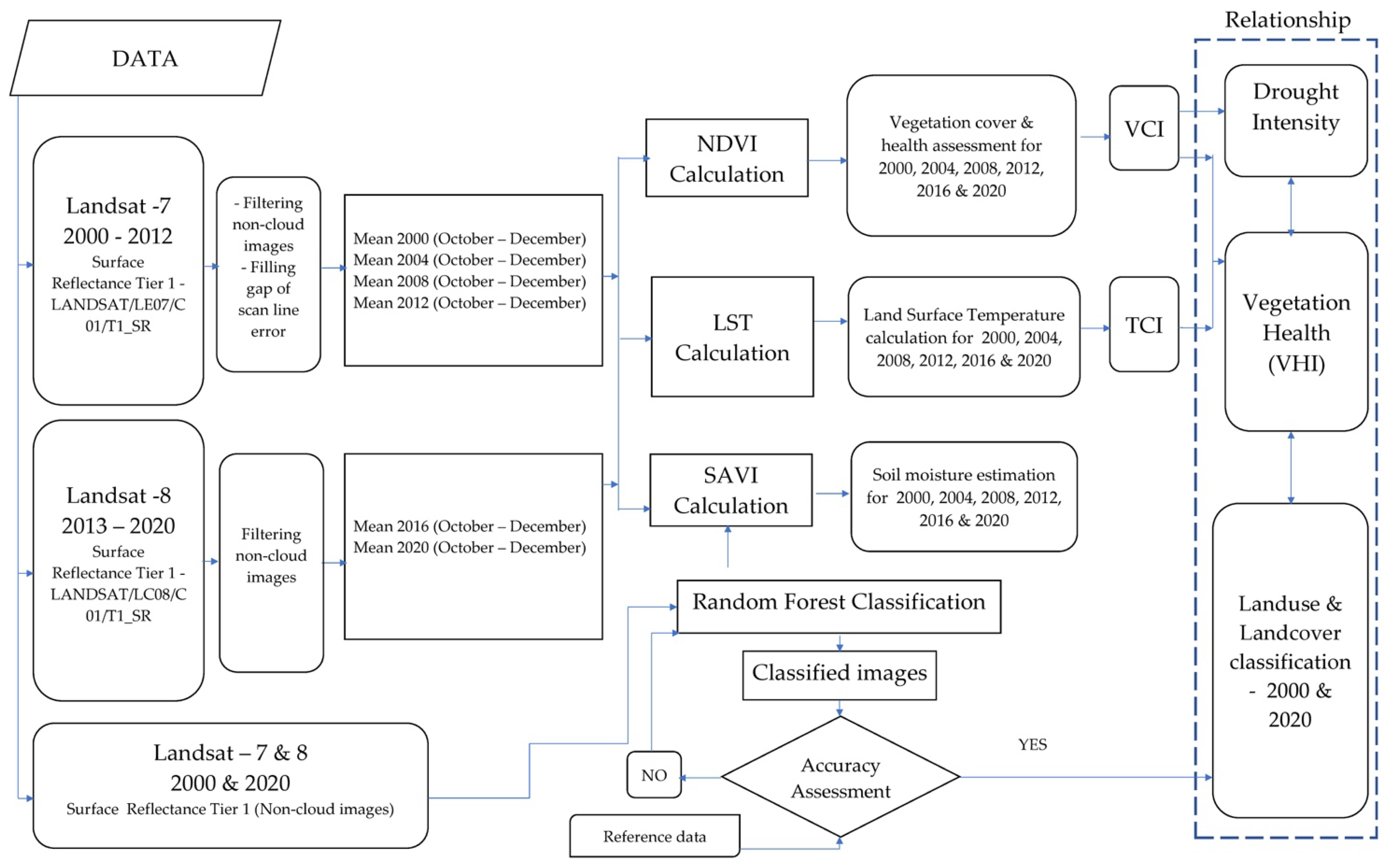
To summarize our research design, we provided a schematic representation for the methodological framework used in this study (Figure 2), which is described in the following subsections.
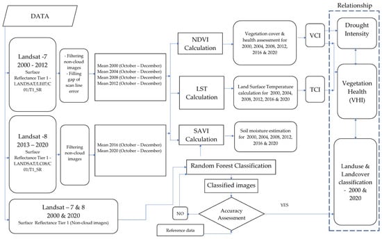
Figure 2.
Methodology for analyzing landscape change and vegetation health (productivity) (NDVI: Normalized Difference Vegetation Index; VCI: Vegetation Condition Index; LST: Land Surface Temperature; TCI: Temperature Condition Index; VHI: Vegetation Health Index; LULC: Land-use and Land cover).
2.3.1. Landuse and Landcover Classification
Land-use classification describes both landuse and landcover (LULC) significantly [32]. LULC change classification helps the policymakers to understand the environmental change dynamics to ensure sustainable development [49]. Therefore, the classification of LULC into different levels is essential [32]. Together, these classification system levels are described as a hierarchy system that is useful in unfolding, monitoring, and forecasting LULC changes [39]. The sources of classifying LULC changes are mainly satellite images and aerial photographs [50,51].
In this study, we analyzed the changes in LULC with seven classes (Table 2) over two decades using Random Forest classification. The Random Forest classification technique is used to enhance the contiguities between the data points. The performance of RF requires the following steps [52,53].
Table 2.
Description of Landuse and Landcover (LULC) classes.
- Developing the N- Tree bootstrap model using satellite imageries.
- Based on DN values, develop an unpruned classification for each bootstrap model.
- In terms of DN values, gather the N-number of polygons.
- Select the number of classifications for land-use classes.
- Generate results of land-use classification.
LULC classification was done in R studio (4.1.3) software based on classes and methods for spatial data, Raster Geospatial Data Abstraction Library (Rgdal), Raster, and Random forests packages [54,55].
The land-use classification results were validated using the GEE images obtained from the year 2000 to 2020. Randomly 75 points were selected, and pixel values of these selected points were extracted for the various study periods. The accuracy assessment performed by comparing land-use classification extracted points with the GEE Image results in identifying those exact points on the GEE. To quantify the accuracy of the results, the kappa coefficient was used in the ERDAS Imagine (8.7) software [56]. The confusion matrix is used in calculating the user and producer accuracies. The kappa coefficient’s accuracy of more than 80% shows the desired land-use classification. Henceforth, the classified results are ancillary to the GEE reference data. The producer accuracy (1), user’s accuracy (2), overall accuracy (3), and Kappa coefficient (4) are calculated using the following Equations [57].
where Obs = Observed Overall accuracy, represents accuracy reported in error matrix, Exp = Expected correct, represents correct classification.
2.3.2. Normalized Difference Vegetation Index (NDVI)
NDVI estimates vegetation by calculating the disparity between infrared, in which vegetation strongly reflects light portions and red light, in which vegetation absorbs light portions [58]. The values of NDVI range from −1 to 1. In this contrast, negative values almost depict the water bodies [59]. On the other hand, the NDVI value near +1 indicates the portion with dense vegetation areas [60]. The value of NDVI around 0 may not be green leaves, which could be urbanized areas [61]. NDVI uses the following Formula (5) to estimate the vegetation areas [61].
where NIR—Near-Infrared Band.
The vegetation with high healthy condition reflects almost close to Near Infrared (NIR) and red in terms of higher different frequencies [58]. The formula results create inducements between the values from −1 to 1 [62]. The indication of low reflectance near red and high reflectance in near-infrared represents the high yield of NDVI [59]. In this study, we extracted NDVI values at regular intervals to differentiate the different growth stages of vegetation productivity and its coverage, i.e., as high productivity, low productivity, and medium productivity. The coverage changes and the productivity of vegetation are quantified using the R packages, Sp, Rgdal, Raster, and rts [54].
2.3.3. Soil Adjusted Vegetation Index (SAVI)
Surface permeability in the study area region was assessed using the Soil Adjusted Vegetation Index (SAVI). In general, SAVI specifies coverage of vegetation and health concerning soil moisture and thus accounts for the high inconsistency of built-up and non-built-up land cover in urban areas [63]. In SAVI, a transformation technique is presented to minimize the effects of external factors from spectral vegetation indices.
SAVI controls for the influence of soil brightness in the NDVI and it reduces the brightness of soil-related noise in the coverage of vegetation estimation [32]. Vegetation health is strongly associated with surface permeability and thus provides an essential identification of impermeable surfaces, especially in urban areas. SAVI is calculated using Equation (6) [32].
where RED is the pixel value of band 3 (RED), and the NIR band is the pixel value of Near-Infrared band 4. L—Soil brightness correction factor [64]. Dense vegetation and high permeable surface areas L = 0, Less vegetation portion and impermeable surface areas L = 1 [65]. Due to the vegetation and coverage of built-up land, the inconsistency level was fixed at L = 0.5 [66].
SAVI
was calculated for the satellite images for the period from 2000 to 2020. The SAVI was extracted at natural breaks to differentiate surface permeability degrees. The computation of area coverage for soil permeability zone between 2000 to 2020 was done using SAVI. For each LULC class, the areal coverage and standard deviation of SAVI are computed.
2.3.4. Land Surface Temperature (LST)
In this study, the LST index was calculated for each pixel in the satellite images from 2000 to 2020 to quantity the radiative skin temperature of the land surface and its elements, which depends on the optical brightness and reflectance of the surface (Albedo) [32]. In general, low SAVI with soil and built-up lands having high albedo [67]. On the other hand, high SAVI with dense vegetation portions has a low albedo, indicating variability in the climatic condition over an urban and dense forest region associated with surface permeability degrees [68]. The LST of each pixel was calculated using Equation (7) [68].
where,
- LMAX = the spectral radiance that is scaled to QCALMAX in W/(m2 *sr *μm)
- LMIN = the spectral radiance that is scaled to QCALMIN in W/(m2 *sr *μm)
- QCALMAX = the maximum quantized calibrated pixel value (corresponding to LMAX) in DN = 255
- QCALMIN = the minimum quantized calibrated pixel value (corresponding to LMIN) in DN = 1
LST was applied to the satellite images for the period from 2000 to 2020. The LST was extracted at natural breaks to differentiate with SAVI. For each LULC class, the areal coverage and standard deviation of LST were computed. Using Spearman correlation analysis, the quantification between the association of surface permeability and LST was achieved.
2.3.5. Vegetation Condition Index (VCI)—Drought Intensity and Temperature Condition Index
Kogan’s vegetation condition index delivers the relative Normalized Difference Vegetation Index changes concerning the historical NDVI pixel values [69]. VHI can be derived based on both the LST and NDVI [70]. It distinguishes the present vegetation index, i.e., NDVI or EVI (Enhanced Vegetation Index), with the values observed in the same data period of different previous years within particular significant pixel values. The VCI calculated as per the Formula (8) [71] shown below
where NDVImax and NDVImin are the maximum and minimum NDVI values for a pixel during a period of time [72]. As a resulting percentage of this formula, Table 3 represents bad to good vegetation conditions in different colors.
Table 3.
Interpretation of the VCI, recommended practice by the United Nations, office for outer space affairs UN—Spider knowledge portal. (Recommended Practice: Drought monitoring using the Vegetation Condition Index (VCI): https://un-spider.org/book/export/html/9206, accessed on 5 January 2020) [73].
2.3.6. Temperature Condition Index (TCI)
The Temperature Condition Index (TCI) proposed by Kogan was used to determine the stress effect on the vegetation possessed by the temperature condition and enormous wetness [74]. The implementation of TCI is anticipated by taking minimum and maximum temperatures and correcting them to project various vegetation types for the different temperature conditions represented by (9) [75]
where LST—Land Surface Temperature, LSTmax, LSTmin—Maximum and Minimum values of Land Surface Temperature.
2.3.7. Vegetation Health Index (VHI)
Vegetation Health Index (VHI) assesses the effectiveness of drought over the area by incorporating vegetation health (i.e.,) lower than average NDVI and higher than the temperature on the vegetation conditions [76,77]. Vegetation Health Condition is the combination of both VCI and TCI written as (10) [78]
where VCI—Vegetation Condition Index, TCI—Temperature Condition Index, and α—parameter which quantifies the involvement of each component in the vegetation health.
3. Results
3.1. Analyzing the Landuse Landcover Changes
Seven LULC classes, namely urban settlements, forest, plantation agriculture, barren land, water bodies, fallow land, and crop-land agriculture, are considered for the analysis, with a spatial extent of about 130,159.46 km2. Analysis of the accuracy of the classified LULC was achieved using user accuracy, producer accuracy, and kappa coefficient using reference data obtained from other sources. Accuracy assessment for 2000 obtained a kappa coefficient of 0.9 with a producer and user accuracy value of 95.62 and 92.15, respectively. For the year 2020, the kappa coefficient is 0.85 and 89.35, 94.16 for producer and user accuracy, respectively (Table 4).
Table 4.
Accuracy assessment for generated LULC map.
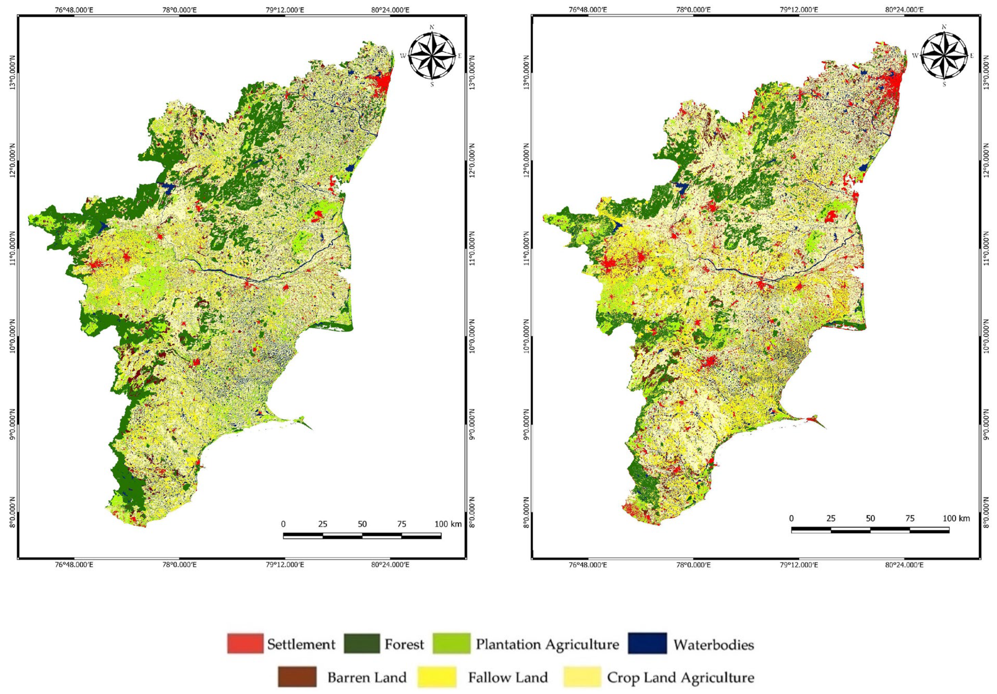
Urban settlements and barren lands increased rapidly by 150% and 120%, respectively, while all other five classes decreased in considerable amounts (Figure 3). The aerial declination of classes forest, plantation-agriculture, water bodies, fallow land, and cropland-agriculture are 21%, 36%, 2%, 14%, and 4%, respectively. The sudden evolution of sub-urban periphery landforms from cropland to impervious constructions was observed, which is depicted as the rapid increase in the settlements as seen in Figure 3 as red patches. Chennai and its fringes had rapid urban development and other sub-urban cities also urbanized due to the migration of the population to cities for various purposes. The barren land also increased by 6477 km2 mainly due to urbanization, leaving the agricultural lands, leading to an increase in uncultivable barren land and water bodies change is around 185 km2, which is at an alarming rate of sign (Table 5). Thus, the landscape of Tamil Nadu is urbanized with the decrease in fertile cropland pastures over the last two decades and the conversion of those lands into barren landforms.
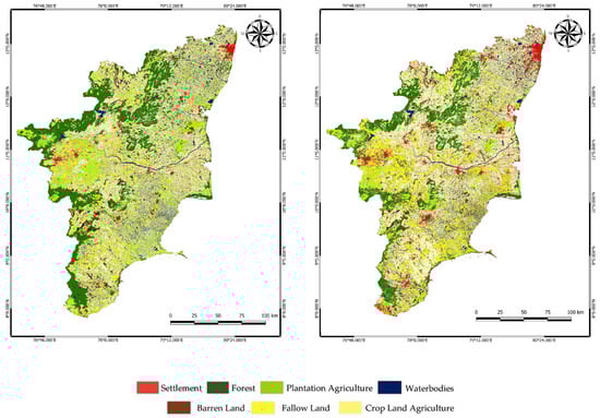
Figure 3.
LULC classification map for 2000 (Left) and 2020 (Right).
Table 5.
Comparative analysis between various classes over two decades.
3.2. Assessment of Vegetation Health
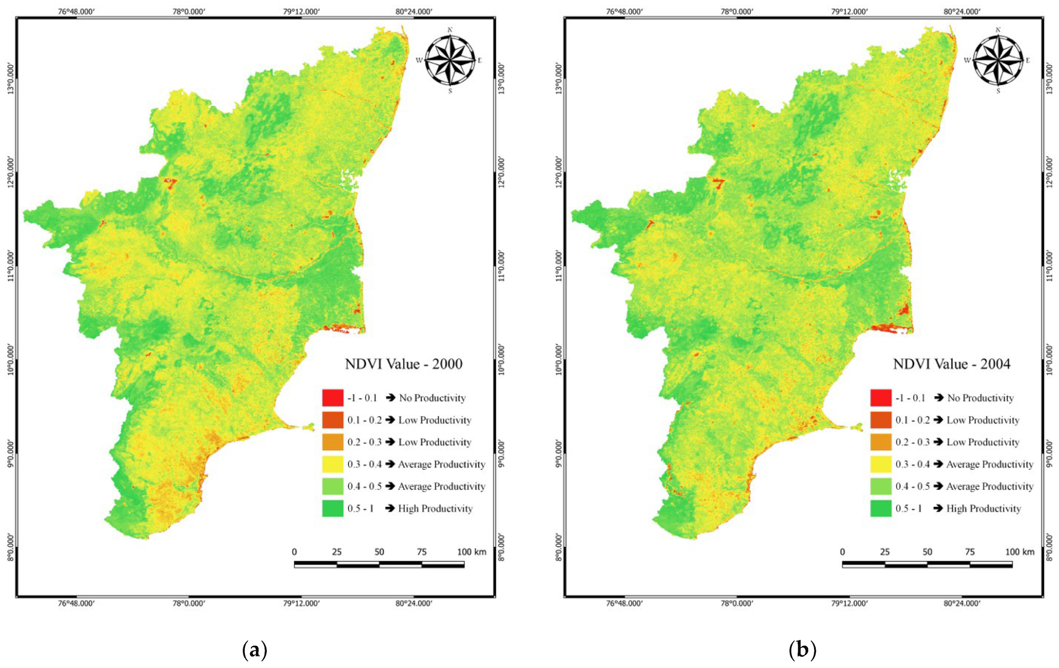
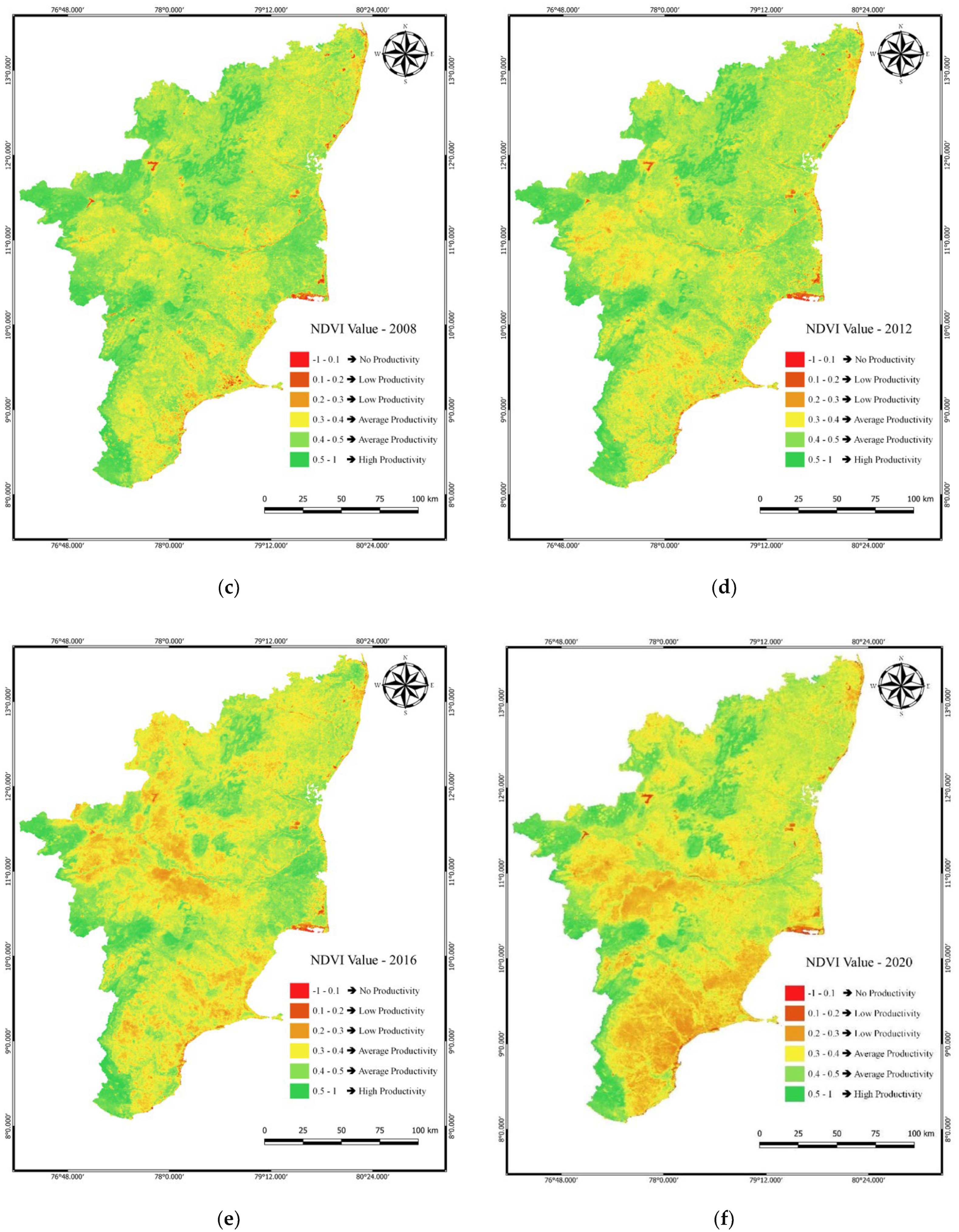
Normalized Difference Vegetation Indices (NDVI) are primarily used to detect the presence of vegetation and the health status of existing plantations. For the analysis carried out over two decades in Tamil Nadu, the plantations are undergoing severe stress and agriculture is becoming difficult as the years pass on. From this study, nearly one-third of the entire area was stress-free in 2000 and the healthy vegetation pattern is clearly visible in river basins because of the high reflectance value in the NIR band (Figure 4). The year 2004 and 2008 has almost the same healthiness in the outpost with slight declination in the landscapes having high productivity compared to that of 2000. In 2012, there was around 50 percent increase in the area ranging between 0.1 to 0.2, which clearly reveals that few plantations are undergoing stress, whereas a lot of agricultural areas are left uncultivated, which is derived from the analysis of high productivity landform changes in comparison with 2008 in which change is around 20%. By comparative analysis of NDVI maps between 2016 and 2020, the southern portion of the study area is undergoing severe stress, as is clearly visible with a decrease in highly productive land by around 45%. From the overall analysis of the healthiness of the vegetation carried over for two decades, we learned that areas with no plantation increased by 218% and low productivity (0.1–0.3) areas increased adversely by about 600% and the average productive land (0.3–0.5) changes around 7.7% and there is a decrease in the healthy regions by about 75% roughly (Table 6). Southern Tamil Nadu has an unhealthy vegetation pattern, while the western portion possesses good healthiness due to the Western Ghats existing in that particular belt.

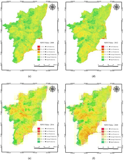
Figure 4.
NDVI map for Tamil Nadu depicting the healthiness of the vegetation (a) 2000, (b) 2004, (c) 2008, (d) 2012, (e) 2016, (f) 2020.
Table 6.
Change in the areal distribution of the NDVI classes for Tamil Nadu for two decades.
3.3. Soil Moisture Assessment
SAVI is the ideal index to assess soil moisture which is evaluated based on the surface permeability. When the SAVI value ranges between −1 to 0.1, then the area may be either water bodies or areas with no soil moisture, i.e., impermeable surfaces; similarly, when the SAVI value increases, the soil moisture tends to increase due to an increase in the soil penetration capability.
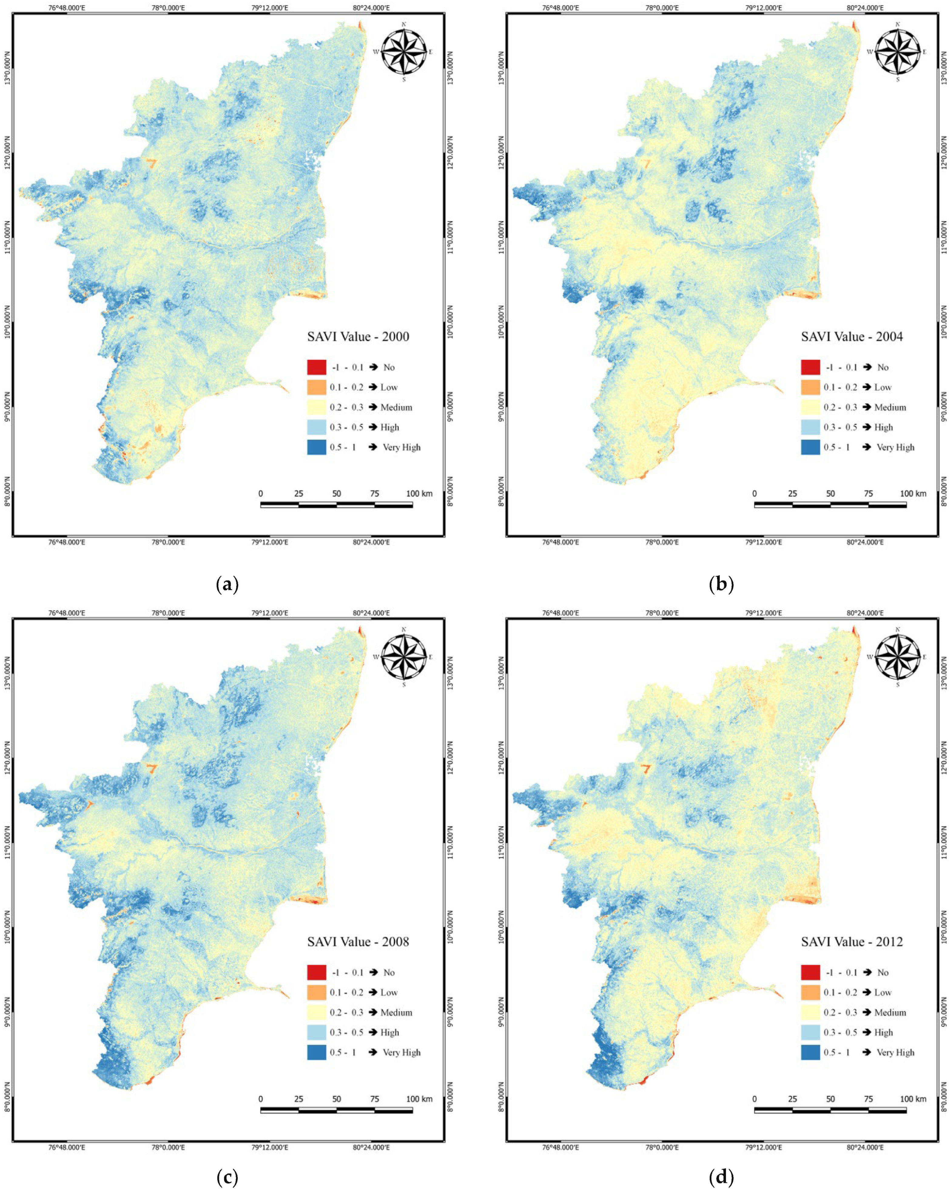
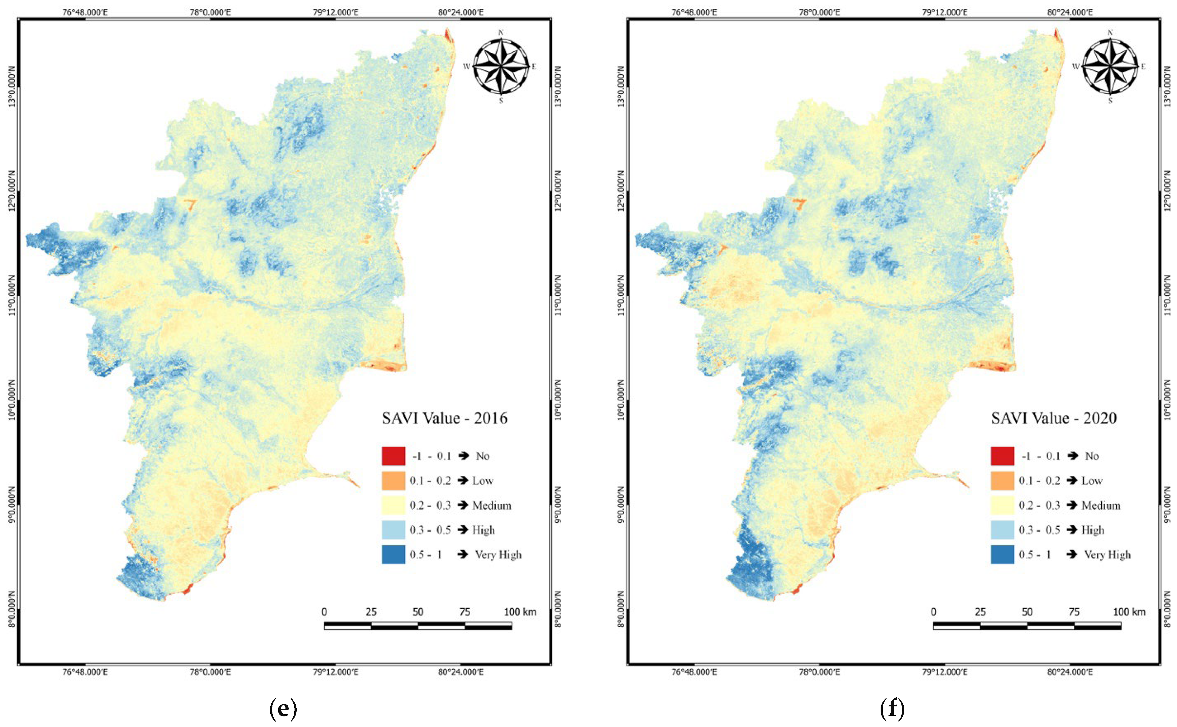
From this analysis, due to the population explosion, deterioration of soil moisture was observed, which is mainly due to an increase in impermeable surfaces. In 2000, nearly 40% of Tamil Nadu had high to very high soil moisture, which was spatially scattered over the state (Figure 5). Similarly, in 2004, very high-high soil moisture areas diminished to 20% and are seen in the Western Ghats and along the water sources. By 2008, soil moisture regained around 35% and there was a considerable rise in the areas having no permeability. Again in 2012, soil moisture deteriorated, which resulted in the increase in areas having medium soil moisture. This leads to stress in the vegetation. From 2012, soil moisture followed a decreasing trend only, i.e., high soil moisture areas get converted into low to no moisture areas. In 2020, nearly 90% of the area fell in the no-medium soil moisture range. By the comparative study of SAVI between 2000 and 2020, areas with no permeability increased by 27.67% and an increase of 76.57% and 107.91% for low and medium permeable areas, respectively, whereas the high and very high permeable areas decreased by 79.41% and 69.52%, respectively (Table 7). The southeast coastal areas of Tamil Nadu are facing continuous declination of soil moisture and a similar trend is visualized in the northwestern parts also.
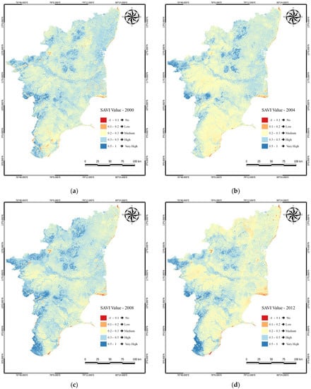
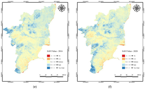
Figure 5.
SAVI map for Tamil Nadu depicting the soil moisture related with permeability (a) 2000, (b) 2004, (c) 2008, (d) 2012, (e) 2016, (f) 2020.
Table 7.
Change analysis of soil moisture for Tamil Nadu for two decades between 2000–2020.
3.4. Calculating Land Surface Temperature
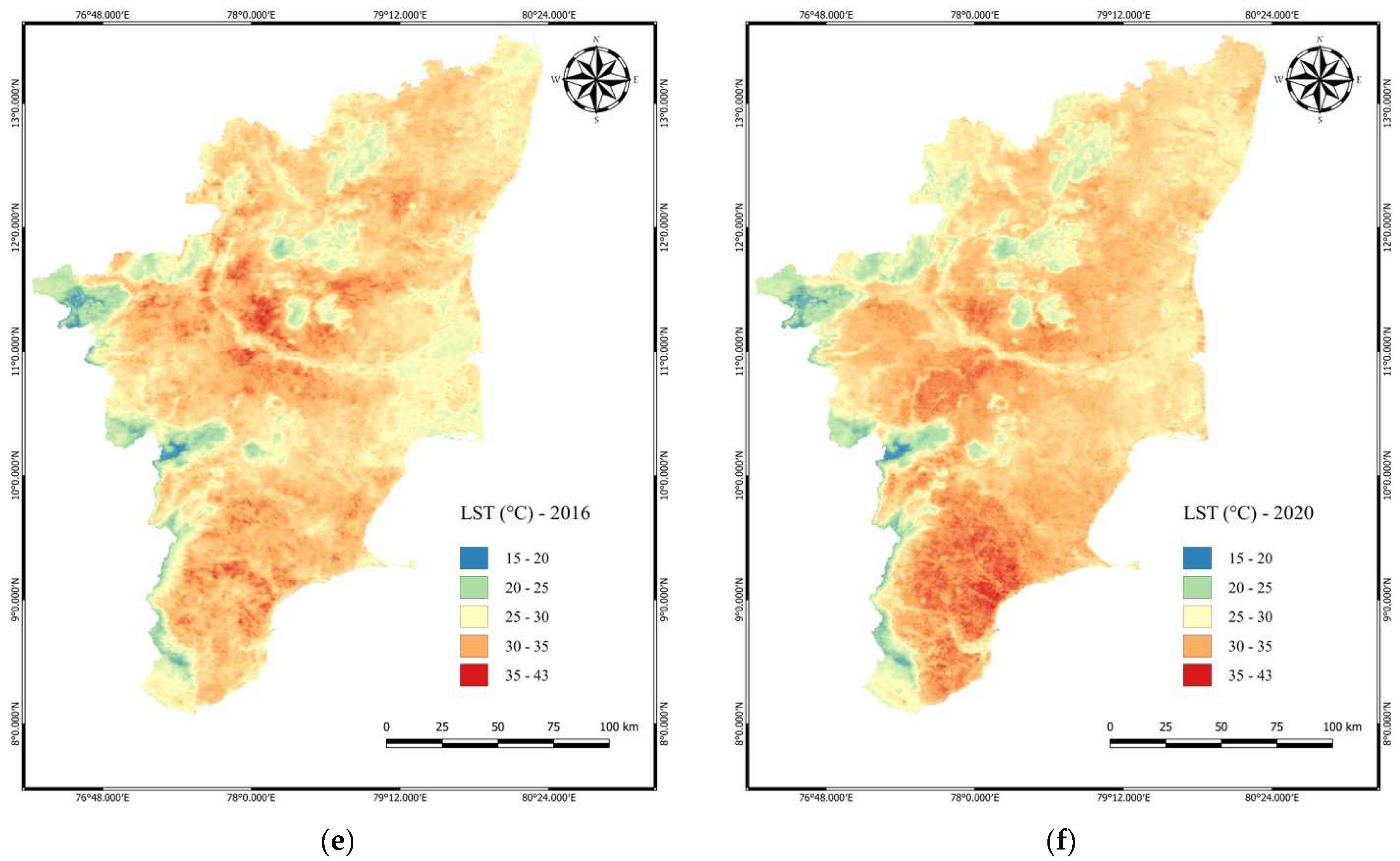
LST is an important parameter related to urban expansion, which increases due to an increase in the terrain temperature. In 2000, the average LST ranges between 18–23 °C and the emissivity was more in the southern part as these areas had a higher LST of around 40 °C and most of the coastal areas in the northern part of Tamil Nadu and the western regions registers an LST between 25–30 °C (Figure 6). By 2004, the LST average in Tamil Nadu declined to a few degrees due to the decrease in LST in the southern part. After 2004, due to various factors like urbanization and industrialization, LST kept on increasing gradually, with the interior parts of Tamil Nadu experiencing a severe rise in LST. Between 2008–2012, there was a bump in the trend in the entire study area, with a 30% increase in the range between 35–42 °C and a decrease in the range between 15–20 °C by 28%. In 2016, it also followed a similar trend with increased LST in the sub-urban areas except the Western Ghats running in the western portions of Tamil Nadu. In 2020, again, the LST increased by 10% in the range of 35–42 °C and around a 147% decrease in the area ranging between 15–25 °C. Thus, the time series analysis of LST reveals that there has been an increase in the LST over two decades enormously due to various reasons and conditions that prevail. An increase in area by 282% with an LST of more than 35 °C observed and 12.46% and 31.66% increases in temperature ranging between 25–30 °C and 30–35 °C, respectively, whereas LST ranging between 15–20 °C and 20–25 °C decreased by 66% and 68%, respectively (Table 8). The areas with mountainous regions also faced a rise in LS in the interior and the southern part experiences severe climatic changes due to urban expansion and a decrease in green cover.
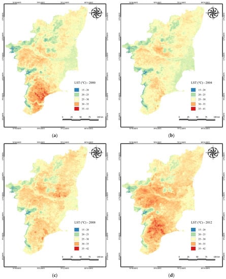
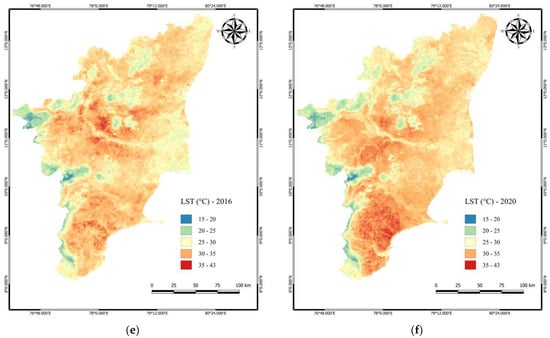
Figure 6.
LST map for Tamil Nadu representing the terrain temperature over two decades (a) 2000, (b) 2004, (c) 2008, (d) 2012, (e) 2016, (f) 2020.
Table 8.
Change analysis of LST for Tamil Nadu for two decades between 2000–2020.
3.5. Comparative Study between NDVI, SAVI, and LST Associated with Each LULC Class
In general, SAVI and NDVI are positively correlated, while the LST has a negative correlation with these two indices. Analysis of the Spearman coefficient reveals that settlements exhibit the highest coefficient value of 0.0061 with the increase in coefficient values (Table 9). This is because urban areas have fewer plantations and very low permeability, which has led to an increase in LST for two decades in Tamil Nadu. Forest and water bodies have the least coefficient values due to healthy dense green cover and high moisture content. The correlation values tend to increase from 2000 to 2020 because of a decrease in plantation and an increase in impervious layer concentration in Tamil Nadu. Thus, to avoid the consequences of LST changes, planners and administrators should focus on increasing the green cover in urban areas where surface permeability is low to avoid the impactful effect on ecosystem services.
Table 9.
Spearman correlation between Normalized Difference Vegetation Indices (NDVI), Soil-adjusted vegetation index (SAVI), and land surface temperature (LST) by landuse and landcover (LULC) zones. All correlation coefficients are statistically significant at p ≤ 0.01.
3.6. Assessing the Drought Intensity for 2020
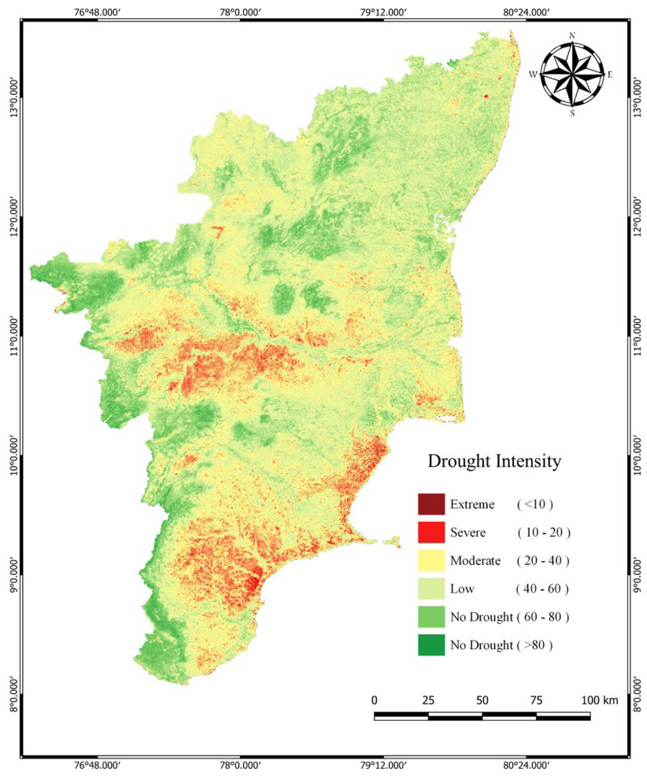
Tamil Nadu experiences a tropical climate, which receives rainfall from monsoons or cyclones, depressions prevailing in the Bay of Bengal. The annual vegetation cycle of Tamil Nadu primarily depends on the southwest and northeast monsoon. If any failure in the monsoon occurs, then disaster begins. VCI is the commonly used index to portray the impacts of drought on vegetation irrespective of the climatic variations. When the VCI value exceeds 60, then crops sustain no impacts due to drought and when it falls below 20, severe impacts occur. In Tamil Nadu, during the year 2020, the drought-prone areas like southern coastal districts and a few western interior districts experience severe impacts due to drought leading to a subsequent deficit in crop yield. The northern districts and Western Ghats (VCI > 60) experience no vegetation stress and vegetation remains healthy because monsoon in those particular regions onset at the correct timeframe and provides enough rainfall for crops. The moderate drought occurs primarily in the outer fringes of severe drought-affected regions and certain riparian parts of the Cauvery deltaic regions, with VCI values ranging between 20 to 60 (Figure 7).

Figure 7.
VCI map (drought intensity map) of Tamil Nadu for 2020.
3.7. Monitoring the Vegetation Health by VHI
Vegetation health generally depends upon the water availability for the survival of the vegetation prevailing. Water availability, i.e., soil moisture that is related to surface temperature, is also considered the major factor for deriving the health index. VHI also considers the VCI, which is related to stress either because of water availability or stress due to diseases that exist in the crop. VHI analyses of all the aforementioned conditions and mapping of the health of the crop, almost 35% of Tamil Nadu has stressed vegetation distribution, and the Western Ghats have healthy vegetation characteristics because of healthy vegetation circumstances and high moisture content (Figure 8). In the case of a failed monsoon, VHI can be improved by providing water supply to crops in the correct proportion by implementing precision agriculture methodologies or changing the irrigation pattern to avoid stress.
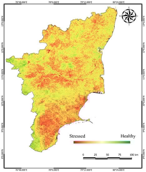
Figure 8.
Analyzing the vegetation health in 2020 using VHI for Tamil Nadu.
3.8. Comparative Study between VCI, VHI, and LST Associated with Each LULC Class
Indices related to vegetation like VCI and VHI are positively correlated, while the LST is negatively correlated to that of the vegetation indices. Drought is the primary causative factor for increasing LST, as clearly portrayed; as drought leads to the decline of crop health, this will result in the emergence of LST. The settlement has the highest spearman coefficient values of 0.0064 with increases in coefficient values of −0.31 and −0.54 for 2000 and 2020, respectively, while the forest has the minimal correlation of 0.0012 among all the LULC classes considered for our analysis (Table 10). Cropland and plantation have almost similar correlation values due to their similar characteristics. However, the correlation values for each class increased from 2000 to 2020 due to urbanization and a decrease in green cover resulting in increased LST.
Table 10.
Spearman correlation between Vegetation Condition Index (VCI), Vegetation Health Index (VHI), and Land Surface Temperature (LST) by landuse and landcover (LULC) zones. All correlation coefficients are statistically significant at p ≤ 0.01.
4. Discussion
Our study on LULC changes in Tamil Nadu over two decades reveals that there is abundant growth in urban areas and fallow landscapes monotonically, about 150% and 120%, respectively, and shrinkage in cropland and plantation agriculture landforms by a notable margin. These changes are mainly due to the movement of people from the rural areas to the towns in Tamil Nadu, notably Chennai, Coimbatore, Trichy, and Madurai, seeking employment by leaving their owning premises, which results in the conversion of agricultural lands into fallow lands and similarity due to high demand urban-fringes are plotted and sold, leading to increase in settlements results in urbanization [25].
Due to the boom in construction, there is an increase in the percentage of impervious layers in landforms, which leads to several other consequences like reduction in green cover, degradation of groundwater, and saltwater intrusion in coastal belts [79], for example, Vedanta Sterlite copper industry (currently closed for violating environmental measures) in Tuticorin and thermal power stations in Tuticorin and Ennore extracted millions of gallons of groundwater drives saltwater intrusion and, toxic discharges degrades the groundwater in the coastal belts of Tuticorin and Chennai, respectively [80,81]. Another example, nuclear power plants in Kalpakkam and Kudankulam also degrade the groundwater and environment due to the discharge of heavy metals and other toxic substances [36]. Surface permeability is assessed using SAVI, a modified NDVI index, which shows that the urban areas and fallow lands have very low surface permeability, resulting in an upsurge of LST [42]. From the NDVI map, it is clear that the healthiness of the vegetation deteriorates during the period of study, and the reality is that major basins (Cauvery basin and Thamirabarani basin) experience stress in the plantation growth, due to inadequate water availability. The stopping or delayed release of Cauvery water from Karnataka dam’s by the Karnataka government is also a driving force of water scarcity in the Cauvery basin and several districts of Tamil Nadu [82]. Thanjavur (the rice bowl of Tamil Nadu) residing in the Cauvery delta plain experiences severe degradation in the healthiness of the crop after 2008, which has severe impacts on the economy of the state. Thus, proper planning must be employed in deltaic and basin areas to renovate the agricultural landforms to achieve sustainable development. VHI and VCI are used to show the healthiness of the vegetation in relation to drought and temperature, respectively. When a certain area is influenced by drought, health deteriorates, and rises in temperatures also cause stress in vegetation due to decreases in soil moisture; however, agricultural crops prevail due to water supply provided by farmers from various water sources.
The main consequence of urbanization is global warming, i.e., an increase in earth temperature to a certain degree is clearly envisaged in the LST map; there is a spike in LST values of about 4–5 °C in two decades. Due to deforestation, which minimizes the natural cooling effect, LST may rise further, causing severe health ailments to the people residing in those areas because of the trap of heat energy by the built-up areas and small roads with the added heat from the air conditioners, vehicle discharge still exacerbates the effect [83]. Southern districts like Rameswaram, Thoothukudi, Virudhunagar, Kanyakumari, Sivagangai, and part of Tirupur had the higher LST values in 2020; however, it can be controlled by improving green cover and erecting artificial groundwater recharge structures to enhance the growth of trees in urban areas, thereby, there will be increased chances of rainfall due to a phenomenon called evapotranspiration [4]. Recently, the LST value upsurges in Kanyakumari districts may be due to the conversation of agriculture and farmland into a national highway project implemented by the National Democratic Alliance (NDA) government. Future research should focus on the Kanyakumari district to identify the cause of the sudden increase in LST.
Urban Sprawl (US) is another major influential factor in the conversion of landscapes [84,85]. Urban areas tend to grow on the outer fringes of the major cities, which results in the shrinkage of production landforms and water bodies being encroached upon, leading to severe impacts on ecosystems. Our study showcases the growth of towns from 2000 to 2020 in the fringes; in this process, the people start to reside in those outer fringes and they start facing troubles like lack of infrastructures, sewage treatment, and proper water supply. To avoid those circumstances, proper urban planning and environmental management practices should be done to achieve sustainable development in those areas [27]. With the increase in urban population and unsustainable replacement of green cover into impervious layer results to cause severe ecological and economic damages. Due to urbanization and population rise ESV (Ecosystem Service Value) falls rapidly, which results in a shortage of multi-utility services provided to the people with needs. Due to the conversion of agricultural land to other landscapes, there is a huge loss in ESV and Gross Domestic Product (GDP) of the state between 2000 and 2020 and demand for food grains increases; thus, ESV and GDP should be evaluated in future research. As the transformation of agricultural or forest land into impervious layers is uncontrollable in developing countries, certain norms of regulations should be incorporated strictly on the public to reduce the impacts of the transformation of landforms [31]. Similarly, certain schemes like the Conversion of Cropland to Forest Program (CCFP) can be implemented, and subsidies can be provided to the farmers who are involved in such schemes, which can be helpful for communities who are all switching their location to urban areas due to any reasons and gaining more ecosystem values. The comparative study of various indices using spearman’s coefficient shows that when the vegetation health and soil moisture deteriorate, then the surface temperature increases, and simultaneously the presence of the severity of drought and the health of vegetation deteriorates, then the area is highly susceptible to the upsurge of LST.
The combined approach of RS, geographical information system (GIS), and LULC change the analysis associated with vegetation and temperature change measures provide useful information and efficient methods and modeling landscape changes on vegetation and land surface temperatures in Tamil Nadu. Therefore, this study also contributes several indices and indicators to monitor drought and vegetation health in Tamil Nadu. It also delivers useful information for urban planning and sustainable development as well as mitigation of environmental impact in Tamil Nadu.
5. Conclusions
In this study, the creation of a LULC map using the RF Algorithm for the entire Tamil Nadu to analyze the spatial and temporal pattern of landcover changes and the accuracy of the LULC map was carried out. We found a rapid increase in the urban settlements and barren lands while the agricultural landscape decreased alarmingly due to various anthropogenic activities from 2000 to 2020. Various indices like NDVI, SAVI, LST, VHI, and VCI were derived using RS data for six different years during the last two decades. The NDVI map was used to identify the vegetation health based on reflectance from chlorophyll pigment. Using NIR imagery, soil moisture was studied using SAVI, which identified the regions having low surface permeability and the areas having low moisture.
The increase in LST values reflects the relationship between urbanization and its impacts on climatic conditions. The intensity of drought in Tamil Nadu is depicted by VCI, while VHI is used to deduce the health of vegetation by including the soil moisture with the NDVI, which will be used to portray the emergence of heat islands in future research. LST is inversely related to VHI and VCI, and the Spearman coefficient relationship shows that urban areas are at a higher risk for the evolution of heat islands. To conclude, our study is done primarily to analyze the impact of landscape changes on vegetation and LST, and a relationship is deduced along with the identification of hotspot areas for the emergence of LST in various districts in Tamil Nadu and plan developmental proposals at the landscape level and maintain the economic benefits and ecological gains of the different land cover classes and monitor the region.
Supplementary Materials
The following supporting information can be downloaded at: https://www.mdpi.com/article/10.3390/earth3020036/s1. Figure S1: Enhanced vegetation index (EVI) for Tamil Nadu 2000 and 2020; Figure S2: Surface Urban Heat Island for Tamil Nadu 2020; Figure S3: Temperature conditon index for Tamil Nadu 2020; Figure S4: NDVI difference between 2000 and 2020; Figure S5: EVI difference between 2000 and 2020.
Author Contributions
Conceptualization, M.S. and R.P.; methodology, M.S. and R.P.; software, M.S. and R.P.; validation, M.S., R.P., P.C. and P.M.; formal analysis, M.S., R.P., and P.C.; investigation, M.S., and R.P.; resources, M.S., R.P. and P.C.; data curation, M.S., R.P., P.C. and P.M.; writing—original draft preparation, M.S. and R.P.; writing—review and editing, M.S., R.P.,P.C. and P.M.; visualization, M.S. and R.P.; supervision, R.P. and P.C.; project administration, R.P. and P.C.; funding acquisition, M.S., R.P. and P.C. All authors have read and agreed to the published version of the manuscript.
Funding
This study was partially supported by national funds through FCT (Fundação para a Ciência e a Tecnologia) under the project UIDB/04152/2020 (Centro de Investigação em Gestão de Informação (MagIC)).
Data Availability Statement
The Google earth engine code with data provided in the Supplementary Section.
Conflicts of Interest
The authors declare no conflict of interest.
References
- Ilman, M.; Dargusch, P.; Dart, P.; Onrizal. A historical analysis of the drivers of loss and degradation of Indonesia’s mangroves. Land Use Policy 2016, 54, 10. [Google Scholar] [CrossRef]
- Verburg, P.H.; Kok, K.; Pontius, R.G.; Veldkamp, A. Modeling Land-Use and Land-Cover Change. In Land-Use and Land-Cover Change; Springer: Berlin/Heidelberg, Germany, 2006; pp. 117–135. [Google Scholar]
- Geist, H.; McConnell, W.; Lambin, E.F.; Moran, E.; Alves, D.; Rudel, T. Causes and Trajectories of Land-Use/Cover Change. In Land-Use and Land-Cover Change; Springer: Berlin/Heidelberg, Germany, 2008; pp. 41–70. [Google Scholar]
- Chauhan, N.; Kumar, V.; Paliwal, R. Quantifying the impacts of decadal landuse change on the water balance components using soil and water assessment tool in Ghaggar river basin. SN Appl. Sci. 2020, 2, 60. [Google Scholar] [CrossRef]
- Mundia, C.N.; Aniya, M. Dynamics of landuse/cover changes and degradation of Nairobi City, Kenya. Land Degrad. Dev. 2006, 17, 97–108. [Google Scholar] [CrossRef]
- Hamilton, S.E.; Casey, D. Creation of a high spatio-temporal resolution global database of continuous mangrove forest cover for the 21st century (CGMFC-21). Glob. Ecol. Biogeogr. 2016, 25, 729–738. [Google Scholar] [CrossRef]
- Whitehead, P.G.; Barbour, E.; Futter, M.N.; Sarkar, S.; Rodda, H.; Caesar, J.; Butterfield, D.; Jin, L.; Sinha, R.; Nicholls, R.; et al. Impacts of climate change and socio-economic scenarios on flow and water quality of the Ganges, Brahmaputra and Meghna (GBM) river systems: Low flow and flood statistics. Environ. Sci. Process. Impacts 2015, 17, 1057–1069. [Google Scholar] [CrossRef]
- Ward, K.; Lauf, S.; Kleinschmit, B.; Endlicher, W. Heat waves and urban heat islands in Europe: A review of relevant drivers. Sci. Total Environ. 2016, 569–570, 527–539. [Google Scholar] [CrossRef]
- Tran, H.; Uchihama, D.; Ochi, S.; Yasuoka, Y. Assessment with satellite data of the urban heat island effects in Asian mega cities. Int. J. Appl. Earth Obs. Geoinf. 2006, 8, 34–48. [Google Scholar] [CrossRef]
- Tariq, A.; Shu, H. CA-Markov chain analysis of seasonal land surface temperature and land use landcover change using optical multi-temporal satellite data of Faisalabad, Pakistan. Remote Sens. 2020, 12, 3402. [Google Scholar] [CrossRef]
- Orusa, T.; Orusa, R.; Viani, A.; Carella, E.; Mondino, E.B. Geomatics and EO data to support wildlife diseases assessment at landscape level: A pilot experience to map infectious keratoconjunctivitis in chamois and phenological trends in Aosta Valley (NW Italy). Remote Sens. 2020, 12, 3542. [Google Scholar] [CrossRef]
- Padmanaban, R.; Bhowmik, A.K.; Cabral, P.; Zamyatin, A.; Almegdadi, O.; Wang, S. Modelling urban sprawl using remotely sensed data: A case study of Chennai city, Tamilnadu. Entropy 2017, 19, 163. [Google Scholar] [CrossRef] [Green Version]
- Moody, E.G.; King, M.D.; Schaaf, C.B.; Hall, D.K.; Platnick, S. Northern Hemisphere five-year average (2000-2004) spectral albedos of surfaces in the presence of snow: Statistics computed from Terra MODIS land products. Remote Sens. Environ. 2007, 111, 337–345. [Google Scholar] [CrossRef]
- de Costa Trindade Amorim, M.C. Spatial variability and intensity frequency of surface heat island in a Brazilian city with continental tropical climate through remote sensing. Remote Sens. Appl. Soc. Environ. 2018, 9, 10–16. [Google Scholar]
- Douglas, I. Ecosystems and Human Well-Being. In Encyclopedia of the Anthropocene; Elsevier: Amsterdam, The Netherlands, 2017; Volume 1–5, pp. 185–197. [Google Scholar]
- Li, Z.L.; Tang, B.H.; Wu, H.; Ren, H.; Yan, G.; Wan, Z.; Trigo, I.F.; Sobrino, J.A. Satellite-derived land surface temperature: Current status and perspectives. Remote Sens. Environ. 2013, 131, 14–37. [Google Scholar] [CrossRef] [Green Version]
- Orusa, T.; Borgogno Mondino, E. Landsat 8 thermal data to support urban management and planning in the climate change era: A case study in Torino area, NW Italy. Environ. Sci. 2019, 11157, 4. [Google Scholar]
- Flores, R.J.L.; Pereira Filho, A.J.; Karam, H.A. Estimation of long term low resolution surface urban heat island intensities for tropical cities using MODIS remote sensing data. Urban Clim. 2016, 17, 32–66. [Google Scholar] [CrossRef]
- Ermida, S.L.; Soares, P.; Mantas, V.; Göttsche, F.M.; Trigo, I.F. Google earth engine open-source code for land surface temperature estimation from the landsat series. Remote Sens. 2020, 12, 1471. [Google Scholar] [CrossRef]
- Naughton, J.; McDonald, W. Evaluating the variability of urban land surface temperatures using drone observations. Remote Sens. 2019, 11, 1722. [Google Scholar] [CrossRef] [Green Version]
- Padmanban, R.; Painho, M. Urban Agent Based Model of Urban SlumDharavi, Mumbai, India. J. Earth Syst. Sci. Eng. 2017, 2, 1110. [Google Scholar]
- Dandona, L.; Dandona, R.; John, R.K.; McCarty, C.A.; Rao, G.N. Population based assessment of uveitis in an urban population in southern India. Br. J. Ophthalmol. 2000, 84, 706–709. [Google Scholar] [CrossRef] [Green Version]
- Usmani, G.; Ahmad, N. Health status in India: A study of urban slum and non-slum population. J. Nurs Res. Pract. 2018, 2, 9–14. [Google Scholar]
- Anees, M.M.; Shukla, R.; Punia, M.; Joshi, P.K. Assessment and visualization of inherent vulnerability of urban population in India to natural disasters. Clim. Dev. 2020, 12, 532–546. [Google Scholar] [CrossRef]
- Balk, D.; Montgomery, M.R.; Engin, H.; Lin, N.; Major, E.; Jones, B. Urbanization in India: Population and urban classification grids for 2011. Data 2019, 4, 35. [Google Scholar] [CrossRef] [Green Version]
- Wu, D.C.N.; Banzon, E.P.; Gelband, H.; Chin, B.; Malhotra, V.; Khetrapal, S.; Watkins, D.; Ra, S.; Jamison, D.T.; Jha, P. Health-care investments for the urban populations, bangladesh and india. Bull. World Health Organ. 2020, 98, 19–29. [Google Scholar] [CrossRef]
- Anuradha, B.; Iyappan, L.; Partheeban, P.; Jaganmogan, K.; Hariharasudan, C.; Palanikumar, K. Statistical study on area cultivated in peri-urban and rural tanks during pre and post rehabilitation. Int. J. Agric. Stat. Sci. 2020, 16, 883–888. [Google Scholar]
- Mohanraj, R.; Sathishkumar, M.; Azeez, P.A.; Sivakumar, R. Pollution status of wetlands in urban Coimbatore, Tamilnadu, India. Bull. Environ. Contam. Toxicol. 2000, 64, 638–643. [Google Scholar] [CrossRef]
- Kiruthiga, K.; Thirumaran, K. Effects of urbanization on historical heritage buildings in Kumbakonam, Tamilnadu, India. Front. Archit. Res. 2019, 8, 94–105. [Google Scholar] [CrossRef]
- Samuel, P.; Antonisamy, B.; Raghupathy, P.; Richard, J.; Fall, C.H.D. Socio-economic status and cardiovascular risk factors in rural and urban areas of Vellore, Tamilnadu, South India. Int. J. Epidemiol. 2012, 41, 1315–1327. [Google Scholar] [CrossRef] [Green Version]
- Padmanaban, R.; Karuppasamy, S.; Narayanan, R. Assessment of pollutant level and forecasting water pollution of Chennai coastal, TamilNadu using R. Indian J. Geo-Mar. Sci. 2018, 47, 1420–1429. [Google Scholar]
- Cabral, P.; Feger, C.; Levrel, H.; Chambolle, M.; Basque, D. Assessing the impact of land-cover changes on ecosystem services: A first step toward integrative planning in Bordeaux, France. Ecosyst. Serv. 2016, 22, 318–327. [Google Scholar] [CrossRef] [Green Version]
- Shuangao, W.; Padmanaban, R.; Mbanze, A.A.; Silva, J.M.N.; Shamsudeen, M.; Cabral, P.; Campos, F.S. Using satellite image fusion to evaluate the impact of land use changes on ecosystem services and their economic values. Remote Sens. 2021, 13, 851. [Google Scholar] [CrossRef]
- Padmanaban, R.; Bhowmik, A.K.; Cabral, P. Satellite image fusion to detect changing surface permeability and emerging urban heat islands in a fast-growing city. PLoS ONE 2019, 14, e0208949. [Google Scholar] [CrossRef] [PubMed]
- Su, S.; Xiao, R.; Jiang, Z.; Zhang, Y. Characterizing landscape pattern and ecosystem service value changes for urbanization impacts at an eco-regional scale. Appl. Geogr. 2012, 34, 295–305. [Google Scholar] [CrossRef]
- Charrua, A.B.; Padmanaban, R.; Cabral, P.; Bandeira, S.; Romeiras, M.M. Impacts of the Tropical Cyclone Idai in Mozambique: A Multi-Temporal Landsat Satellite Imagery Analysis. Remote Sens. 2021, 13, 201. [Google Scholar] [CrossRef]
- Mateo-García, G.; Gómez-Chova, L.; Amorós-López, J.; Muñoz-Marí, J.; Camps-Valls, G. Multitemporal cloud masking in the Google Earth Engine. Remote Sens. 2018, 10, 1079. [Google Scholar] [CrossRef] [Green Version]
- Chidambaram, S.; Karmegam, U.; Prasanna, M.V.; Sasidhar, P. A study on evaluation of probable sources of heavy metal pollution in groundwater of Kalpakkam region, South India. Environmentalist 2012, 32, 371–382. [Google Scholar] [CrossRef]
- Kumar, L.; Mutanga, O. Google Earth Engine applications since inception: Usage, trends, and potential. Remote Sens. 2018, 10, 1509. [Google Scholar] [CrossRef] [Green Version]
- Tan, Z.; Guan, Q.; Lin, J.; Yang, L.; Luo, H.; Ma, Y.; Tian, J.; Wang, Q.; Wang, N. The response and simulation of ecosystem services value to land use/land cover in an oasis, Northwest China. Ecol. Indic. 2020, 118, 711. [Google Scholar] [CrossRef]
- Schirpke, U.; Tscholl, S.; Tasser, E. Spatio-temporal changes in ecosystem service values: Effects of land-use changes from past to future (1860–2100). J. Environ. Manag. 2020, 272, 111068. [Google Scholar] [CrossRef]
- Sil, Â.; Fonseca, F.; Gonçalves, J.; Honrado, J.; Marta-Pedroso, C.; Alonso, J.; Ramos, M.; Azevedo, J.C. Analysing carbon sequestration and storage dynamics in a changing mountain landscape in Portugal: Insights for management and planning. Int. J. Biodivers. Sci. Ecosyst. Serv. Manag. 2017, 13, 82–104. [Google Scholar] [CrossRef] [Green Version]
- Xu, P.; Jin, P.; Yang, Y.; Wang, Q. Evaluating Urbanization and Spatial-Temporal Pattern Using the DMSP/OLS Nighttime Light Data: A Case Study in Zhejiang Province. Math. Probl. Eng. 2016, 2016, 890. [Google Scholar] [CrossRef] [Green Version]
- Dewan, A.; Kiselev, G.; Botje, D.; Mahmud, G.I.; Bhuian, M.H.; Hassan, Q.K. Surface urban heat island intensity in five major cities of Bangladesh: Patterns, drivers and trends. Sustain. Cities Soc. 2021, 71, 102926. [Google Scholar] [CrossRef]
- Tang, Q.; Wang, J.; Jing, Z.; Yan, Y.; Niu, H. Response of ecological vulnerability to land use change in a resource-based city, China. Resour. Policy 2021, 74, 102324. [Google Scholar] [CrossRef]
- Nivedita Priyadarshini, K.; Sivashankari, V.; Shekhar, S. An assessment of Land Cover Change Dynamics of Gaja Cyclone in Coastal Tamil Nadu, India Using Sentinel 1 SAR Dataset. In International Archives of the Photogrammetry, Remote Sensing and Spatial Information Sciences—ISPRS Archives; ISPRS: Hannover, Germany, 2019; Volume 42. [Google Scholar]
- Muthusamy, S.; Sivakumar, K.; Durai, A.; Sheriff, M. Ockhi Cyclone and its Impact in the Kanyakumari District of Southern Tamilnadu, India: An Aftermath Analysis. Int. J. Recent Res. Asp. 2018, 1, 466–469. [Google Scholar]
- Bangaru Kamatchi, S.; Parvathi, R. Analysis of timeseries forecasting models using Tamilnadu environmental weather data. J. Green Eng. 2020, 10, 1208–1217. [Google Scholar]
- Kennedy, R.E.; Yang, Z.; Gorelick, N.; Braaten, J.; Cavalcante, L.; Cohen, W.B.; Healey, S. Implementation of the LandTrendr algorithm on Google Earth Engine. Remote Sens. 2018, 10, 691. [Google Scholar] [CrossRef] [Green Version]
- GEE Earth Engine Data Catalog. Available online: https://developers.google.com/earth-engine/datasets/catalog/ (accessed on 4 January 2020).
- Geist, H.; McConnell, W.; Lambin, E.F.; Moran, E.; Alves, D.; Rudel, T. Land-Use and Land-Cover Change; Springer: Berlin/Heidelberg, Germany, 2006. [Google Scholar]
- Breiman, L. Random forests. Mach. Learn. 2001, 45, 5–32. [Google Scholar] [CrossRef] [Green Version]
- Pal, M. Random forest classifier for remote sensing classification. Int. J. Remote Sens. 2005, 26, 217–222. [Google Scholar] [CrossRef]
- Svetnik, V.; Liaw, A.; Tong, C.; Christopher Culberson, J.; Sheridan, R.P.; Feuston, B.P. Random Forest: A Classification and Regression Tool for Compound Classification and QSAR Modeling. J. Chem. Inf. Comput. Sci. 2003, 43, 1947–1958. [Google Scholar] [CrossRef]
- Reichardt, J.; Bornholdt, S. Statistical mechanics of community detection. Phys. Rev. E–Stat. Nonlinear Soft Matter Phys. 2006, 74, 1–27. [Google Scholar] [CrossRef] [Green Version]
- Özçift, A. Random forests ensemble classifier trained with data resampling strategy to improve cardiac arrhythmia diagnosis. Comput. Biol. Med. 2011, 41, 265–271. [Google Scholar] [CrossRef]
- Gao, J. A hybrid method toward accurate mapping of mangroves in a marginal habitat from spot multispectral data. Int. J. Remote Sens. 1998, 19, 1887–1899. [Google Scholar] [CrossRef]
- Islami, F.A.; Tarigan, S.D.; Wahjunie, E.D.; Dasanto, B.D. Accuracy Assessment of Land Use Change Analysis Using Google Earth in Sadar Watershed Mojokerto Regency. IOP Conf. Ser. Earth Environ. Sci. 2022, 950, 9. [Google Scholar] [CrossRef]
- Aubard, V.; Paulo, J.A.; Silva, J.M.N. Long-term monitoring of cork and holm oak stands productivity in Portugal with Landsat imagery. Remote Sens. 2019, 11, 525. [Google Scholar] [CrossRef] [Green Version]
- Ruiz-Luna, A.; Berlanga-Robles, C.A. Modifications in Coverage Patterns and Land Use around the Huizache-Caimanero Lagoon System, Sinaloa, Mexico: A Multi-temporal Analysis using LANDSAT Images. Estuar. Coast. Shelf Sci. 1999, 49, 37–44. [Google Scholar] [CrossRef] [Green Version]
- Bhowmik, A.K.; Cabral, P. Cyclone Sidr Impacts on the Sundarbans Floristic Diversity. Earth Sci. Res. 2013, 2, 62–79. [Google Scholar] [CrossRef] [Green Version]
- Padmanaban, R.; Bhowmik, A.K.; Cabral, P. A remote sensing approach to environmental monitoring in a reclaimed mine area. ISPRS Int. J. Geo-Inf. 2017, 6, 401. [Google Scholar] [CrossRef] [Green Version]
- Son, N.T.; Chen, C.F.; Chen, C.R. Mapping Mangrove Density from Rapideye Data in Central America. Open Geosci. 2017, 9, 18. [Google Scholar] [CrossRef] [Green Version]
- Meza Diaz, B.; Blackburn, G.A. Remote sensing of mangrove biophysical properties: Evidence from a laboratory simulation of the possible effects of background variation on spectral vegetation indices. Int. J. Remote Sens. 2003, 24, 53–73. [Google Scholar] [CrossRef]
- Zhen, Z.; Chen, S.; Yin, T.; Chavanon, E.; Lauret, N.; Guilleux, J.; Henke, M.; Qin, W.; Cao, L.; Li, J.; et al. Using the negative soil adjustment factor of soil adjusted vegetation index (Savi) to resist saturation effects and estimate leaf area index (lai) in dense vegetation areas. Sensors 2021, 21, 2115. [Google Scholar] [CrossRef]
- Rondeaux, G.; Steven, M.; Baret, F. Optimization of soil-adjusted vegetation indices. Remote Sens. Environ. 1996, 55, 95–107. [Google Scholar] [CrossRef]
- Huete, A.R. A soil-adjusted vegetation index (SAVI). Remote Sens. Environ. 1988, 25, 295–309. [Google Scholar] [CrossRef]
- Jung, M.C.; Dyson, K.; Alberti, M. Urban Landscape Heterogeneity Influences the Relationship between Tree Canopy and Land Surface Temperature. Urban For. Urban Green. 2021, 57, 126930. [Google Scholar] [CrossRef]
- Batbaatar, J.; Gillespie, A.R.; Sletten, R.S.; Mushkin, A.; Amit, R.; Liaudat, D.T.; Liu, L.; Petrie, G. Toward the detection of permafrost using land-surface temperature mapping. Remote Sens. 2020, 12, 695. [Google Scholar] [CrossRef] [Green Version]
- Pei, F.; Wu, C.; Liu, X.; Li, X.; Yang, K.; Zhou, Y.; Wang, K.; Xu, L.; Xia, G. Monitoring the vegetation activity in China using vegetation health indices. Agric. For. Meteorol. 2018, 248, 215–227. [Google Scholar] [CrossRef]
- Möllmann, J.; Buchholz, M.; Kölle, W.; Musshoff, O. Do remotely-sensed vegetation health indices explain credit risk in agricultural microfinance? World Dev. 2020, 127, 104771. [Google Scholar] [CrossRef] [Green Version]
- Liang, L.; Sun, Q.; Luo, X.; Wang, J.; Zhang, L.; Deng, M.; Di, L.; Liu, Z. Long-term spatial and temporal variations of vegetative drought based on vegetation condition index in China. Ecosphere 2017, 8, e01919. [Google Scholar] [CrossRef]
- Dutta, D.; Kundu, A.; Patel, N.R.; Saha, S.K.; Siddiqui, A.R. Assessment of agricultural drought in Rajasthan (India) using remote sensing derived Vegetation Condition Index (VCI) and Standardized Precipitation Index (SPI). Egypt. J. Remote Sens. Space Sci. 2015, 18, 53–63. [Google Scholar] [CrossRef] [Green Version]
- Un-spider.org. Recommended Practice: Drought Monitoring Using the Vegetation Condition Index (VCI). Available online: https://www.un-spider.org/advisory-support/recommended-practices/recommended-practice-drought-monitoring-using-vegetation (accessed on 4 January 2022).
- Wang, L.; Wang, P.; Liang, S.; Qi, X.; Li, L.; Xu, L. Monitoring maize growth conditions by training a BP neural network with remotely sensed vegetation temperature condition index and leaf area index. Comput. Electron. Agric. 2019, 160, 82–90. [Google Scholar] [CrossRef]
- Tian, M.; Wang, P.; Khan, J. Drought forecasting with vegetation temperature condition index using arima models in the guanzhong plain. Remote Sens. 2016, 8, 690. [Google Scholar] [CrossRef] [Green Version]
- Bento, V.A.; Gouveia, C.M.; DaCamara, C.C.; Libonati, R.; Trigo, I.F. The roles of NDVI and Land Surface Temperature when using the Vegetation Health Index over dry regions. Glob. Planet. Change 2020, 190, 103198. [Google Scholar] [CrossRef]
- Amalo, L.F.; Hidayat, R.; Sulma, S. Analysis of agricultural drought in east java using vegetation health index. Agrivita 2018, 40, 63–73. [Google Scholar] [CrossRef] [Green Version]
- Bento, V.A.; Gouveia, C.M.; DaCamara, C.C.; Trigo, I.F. A climatological assessment of drought impact on vegetation health index. Agric. For. Meteorol. 2018, 259, 286–295. [Google Scholar] [CrossRef]
- National Ground Water Association. Ground Water Sustainability: A White Paper; National Ground Water Association: Westerville, OH, USA, 2004; pp. 1–13. [Google Scholar]
- Selvam, S.; Venkatramanan, S.; Singaraja, C. A GIS-based assessment of water quality pollution indices for heavy metal contamination in Tuticorin Corporation, Tamilnadu, India. Arab. J. Geosci. 2015, 8, 10611–10623. [Google Scholar] [CrossRef]
- Nath, A. Sterlite Copper Plant in Tuticorin to Remain Closed, Orders Madras HC. Available online: https://www.indiatoday.in/india/story/vedanta-sterlite-copper-plant-tuticorin-madras-high-court-1712406-2020-08-18 (accessed on 4 January 2022).
- The Times of India. Available online: https://timesofindia.indiatimes.com/ (accessed on 4 January 2022).
- Myers, S.S. Global environmental change: The threat to human health. Political Sci. 2009, 2009, 824. [Google Scholar]
- Costanza, R.; d’Arge, R.; De Groot, R.; Farber, S.; Grasso, M.; Hannon, B.; Limburg, K.; Naeem, S.; O’neill, R.V.; Paruelo, J.; et al. The value of the world’s ecosystem services and natural capital. Ecol. Econ. 1998, 25, 3–15. [Google Scholar] [CrossRef]


Publisher’s Note: MDPI stays neutral with regard to jurisdictional claims in published maps and institutional affiliations. |
© 2022 by the authors. Licensee MDPI, Basel, Switzerland. This article is an open access article distributed under the terms and conditions of the Creative Commons Attribution (CC BY) license (https://creativecommons.org/licenses/by/4.0/).