FischerLab: An Application for Generating Fischer Plots and Dynamic Fischer Plots from Wireline Well-Logs and Stratigraphic Data

Abstract

Fischer plots are a technique that is used to graph changes in accommodation in cyclic carbonate successions. They typically depict the cumulative departure from the average cycle thickness as a function of the cycle number or stratigraphic depth. Many applications of Fischer plots focus on their construction from exposed cyclic carbonate successions. No published programs allow the direct construction of Fischer plots from digital wireline well-logs or dynamic presentations of Fischer plots. Here, we introduce a program known as FischerLab, which facilitates the generation and analysis of Fischer plots. In addition to accepting interpreted stratigraphic data input, FischerLab facilitates the interpretation of digital wireline logs for the generation of Fischer plots in cycle and depth domains, as well as in a dynamic evolving cycle and relative depth domain from an easy-to-use interface. The dynamic construction facilitates the correlation of specific stratigraphic packages to parts of the accommodation cycle while simultaneously tracking the locus of the mean subsidence vector. We demonstrate the use of FischerLab on data derived from the carbonate succession outcrops of the Al-Athrun Formation, Libya, and the Glen Rose Formation, Central Texas, USA, as well as on wireline well-log data from the Western Great Bahama Bank, the Bahamas.

1. Introduction

Fischer plots are diagrams that depict the change in accommodation derived from the aggradational stacking patterns in cyclic carbonate successions composed of multiple genetic cycles. Fischer [1] introduced the concept of the diagram to explain the variation in the thickness and observed megacycles of peritidal Triassic Lofer cyclothems of the calcareous Alps. The study originally labeled the vertical axes as ‘vertical space’ and the horizontal axes as ‘time.’ The plots display a cumulative departure from the mean cycle thickness plotted against the cycle number. For each individual cycle thickness, the average cycle thickness is subtracted. This results in positive and negative slopes that are respectively interpreted as increases and decreases in accommodation [2]. To take into account the construction and assumptions of Fischer plots and poor absolute geological time control, Sadler et al. [2] suggested the more appropriate labels of ‘cumulative departure from mean cycle thickness’ and ‘cycle number’ for the vertical and horizontal axes, respectively. Fischer plots are useful tools for the investigation of the variation of thickness within a cyclic carbonate succession. In the depth domain, the Fischer plot can be placed alongside wireline logs or stratigraphic columns, as shown by [3], making the assumption of equal cycle duration unnecessary while providing a single framework for the analysis of stratigraphic data.

Fischer plots are typically applied to cyclic carbonate successions. Peritidal carbonates are deposited in shallow-water environments, and are volumetrically significant on modern and ancient carbonate platforms [4]. In peritidal strata, subtidal, intertidal and supratidal facies are arranged into asymmetric, shallowing-upwards cyclothems or parasequences [5]. The internal architecture and the origin of the cyclicity of carbonate platforms have been widely studied [6,7,8]. Wilkinson et al. [9] and Drummond and Dugan [10] modeled and demonstrated how these cyclic patterns and bed thicknesses could develop. Fischer plot trends display large-scale sequences that can be used to define transgressive and highstand systems tracts and diagnostic intervals [11].

Here, we present FischerLab, a new program for the plotting and analysis of Fischer plots. Read and Sririam [12] and Husinec et al. [13], respectively, presented a VS Fortran (version 2.0) code and an Excel spreadsheet for the construction of Fischer plots. Similar to Read and Sririam [12], Husinec et al. [13] simplified the input procedure and required input data for cycle thickness and the number of covered intervals. The improvement introduced by FischerLab over previous Fischer plot programs is that FischerLab facilitates the direct interpretation of wireline well-logs. In addition, FischerLab produces Fischer plots in the cycle and stratigraphic depth domains, as well as in an evolving cycle and a relative stratigraphic depth domain, wherein the relative stratigraphic depth is simply a stratigraphic distance relative to an arbitrary point. Dynamic construction facilitates the interpretation of the Fischer plots and the correlation of parts of a stratigraphic succession with cycles of the Fischer plot in order to investigate which accommodation regime corresponds to each genetic package. Dynamic Fischer plot analysis also depicts the subsidence history of the succession by tracking the locus of the mean subsidence vector as each new cycle is added.

2. Description of Fischer Plots

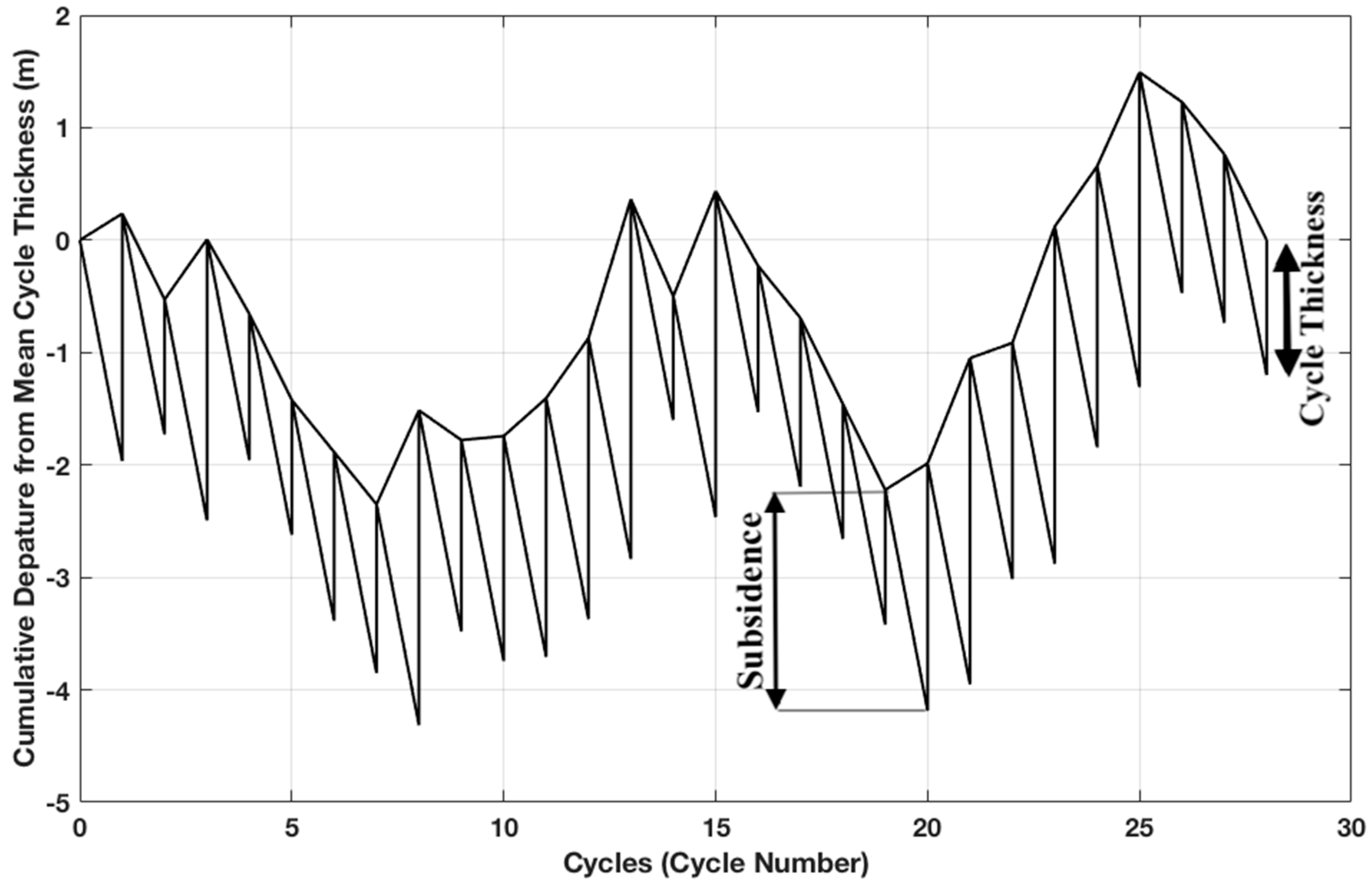
Fischer plots are constructed from stacked cyclic carbonate sections by representing the thickness of each cycle as a vertical line. The next cycle is shifted to the right and down by a single cycle unit and the average thickness, respectively (Figure 1). The shift to the right represents the cycle duration, while the shift down represents subsidence (it could also include corrections for compaction or isostasy). These fundamental parameters result from the simplified assumptions of fixed cycle duration and linear subsidence. The line connecting the top of the cycles forms a wave train that starts at zero and ends at zero, because the cycles thicker than the mean contribute a positive slope, while the cycles that are thinner than the mean contribute a negative slope. In the depth domain, the duration of each Fischer plot cycle corresponds to the exact stratigraphic cycle duration or thickness. In this case, the cumulative departure from the mean thickness (CDMT) is the difference between the actual depth and the depth that the cycle top would have occurred at if all of the cycles were of the same thickness, as given by Day [3]. It can be expressed as follows:

$${\mathrm{CDMT}}_{\mathrm{i}}=\left({\mathrm{D}}_0-\frac{\mathrm{i}}{\mathrm{N}}\mathrm{T}\right)-{\mathrm{D}}_{\mathrm{i}}\mathrm{i}=1..\mathrm{N}$$

(1)

where i is the cycle number and ranges from 1 to N, starting from the deepest; D_i is the depth at the top of the ith cycle; D₀ is the depth at the base of the first cycle; N is the number of cycles; and T is the total thickness.

The dynamic Fischer plot shows the transition of the Fischer plot in the cycle domain, together with the transition of the stratigraphic section in a relative depth domain. Following the assumptions of the Fischer plot, the cyclic packages that have already being deposited are subjected to subsidence equal to the mean thickness of all of the stratigraphic cycles in the section, creating accommodation for the next cycle to be deposited at the top. The mean subsidence vector is the line connecting the base of the stratigraphic section to the beginning of the first cycle of the Fischer plot. This implies that the slope of the line increases as more cycles are deposited, and the stratigraphic section subsides. The dynamic Fischer plot tracks this change in slope as well as the change in the slope of the subsidence vector of each individual cycle (see the Supplementary file list in

Table A1. Supplementary file information.

Filename	Description
Fischerlab_demonstration.avi	Video demonstration of FischerLab usage
fischerlab_movie_ODP_LEG166_1003_from_GR_Log_Bahamas.gif	Dynamic Fischer plot derived from gamma-ray and resistivity wireline logs from the Ocean Drilling Program (ODP) Leg 166, Site 1003 in gif format. (Can be viewed with most browsers)
fischerlab_movie_ODP_LEG166_1003_from_GR_Log_Bahamas.avi	Dynamic Fischer plot derived from gamma-ray and resistivity wireline logs from the Ocean Drilling Program (ODP) Leg 166, Site 1003 in avi format
fischerlab_movie_Al-Athrun.gif	Dynamic Fischer plot derived from the Al-Athrun Formation, Libya, in gif format. (Can be viewed with most browsers)
fischerlab_movie_Al-Athrun.avi	Dynamic Fischer plot derived from the Al-Athrun Formation, Libya in avi format

in the Appendix A for dynamic Fischer plot examples).

Use of Fischer Plots

Fischer plots were initially introduced as a technique for the study of the vertically stacked, meter-scale, shallowing-upward, alternating sequences of subtidal and peritidal deposits that built up carbonate platforms to hundreds of meters. This system of alternating sediments requires repetitive accumulation processes that are independent of geological time [14]. Fischer proposed small-scale glacio-eustatic sea-level oscillations controlled by Milankovitch climatic cycles as the causal mechanism. Sequence stratigraphic principles, however, apply at varying temporal and spatial scales, although the correct methodology to use is dependent primarily on the temporal and spatial scale of the stratigraphic interval and the area under consideration [15,16]. It follows that, in addition to the Milankovitch cycle scale, Fischer plots can be applied on a varying range of scales; for example, the technique has been applied to extract long-term relative sea-level changes from carbonate successions [7,17] and in the analysis of parasequence stacking patterns.

Controversies have surrounded the use of Fischer plots regarding the subjective nature of cycle picks [8,18], which may depend on the stratigrapher’s judgment. However, this issue has been extensively addressed by Sadler [2]. The algorithm and methods of constructing Fischer plots themselves are objective and reproducible, require no information about age and subsidence, and can be used to identify stacking patterns in any facies succession [2]. Moreover, Sadler et al. [2] demonstrated that the gross form of the Fischer plot is preserved when a few subjective cycle picks are involved, and that the overall form of the Fischer plot is not affected by a few variations in cycle picks. To further address this issue, Husinec et al. [13] recommended making Fischer plots for multiple sections. A correlation between the Fischer plots of multiple sections can then be used to document the changes in accommodation.

3. FischerLab Description and Use

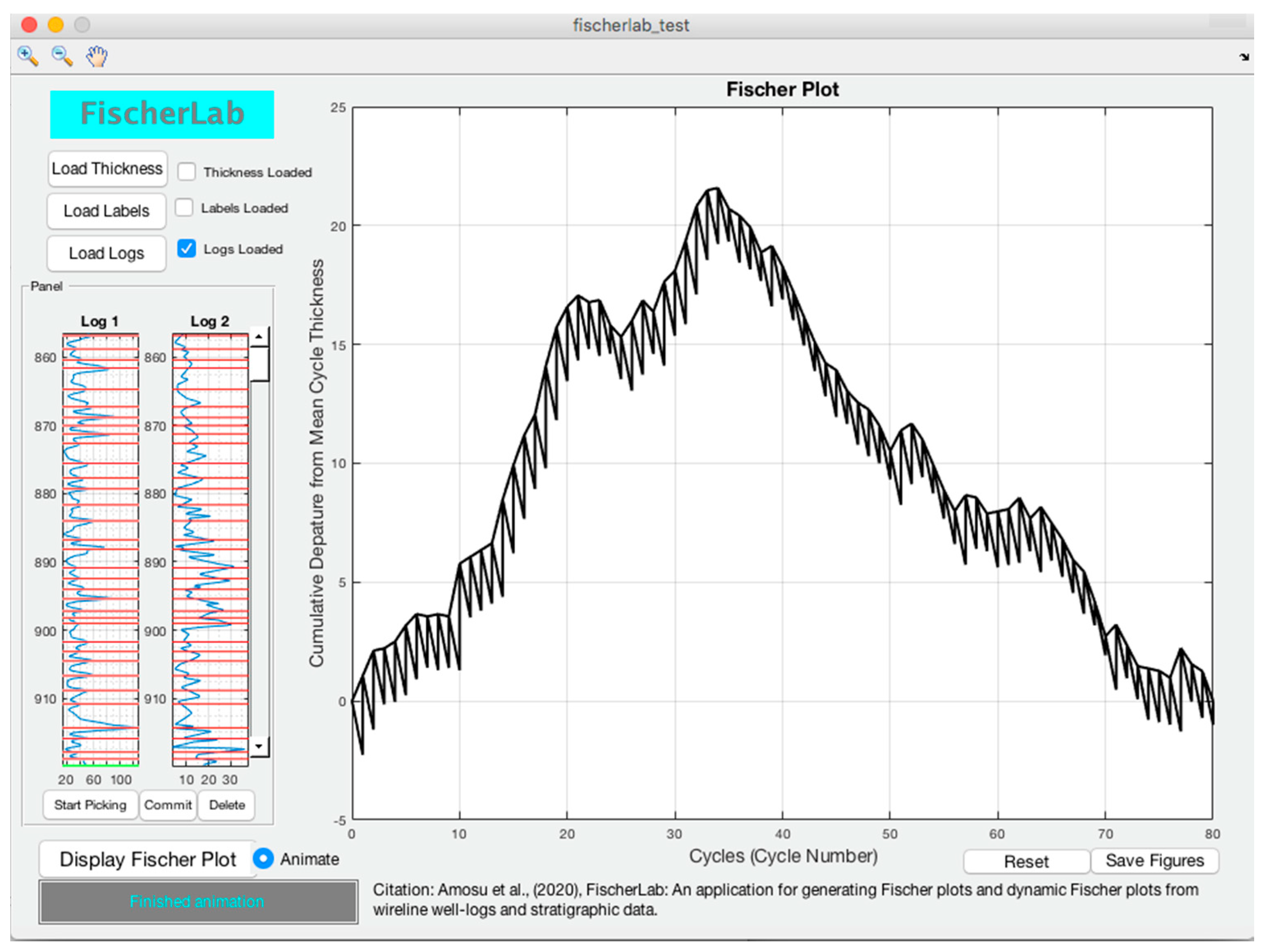
FischerLab [19] was written in MATLAB, and can be deployed as a MATLAB graphical user interface (GUI) application (Figure 2). A description for the use of FischerLab is given below, and a demonstration of the program is given in a Supplementary video file provided with this paper (see the Supplementary file list in Table A1).

The program permits the inputting of data in different formats. Three buttons are used to load data: the ‘Load Thickness,’ ‘Load Labels,’ and ‘Load Logs’ buttons. The ‘Load thickness’ button accepts interpreted cycle thicknesses and facies names in a comma-separated values (CSV) format, Excel’s open XML (XSLX) spreadsheet format, or American Standard Code for Information Interchange (ASCII text) format (only when loading thickness values in a separate file). The ‘Load Labels’ button is reserved primarily for loading facies information in ‘ASCII text’ format if the thickness data is loaded in ‘ASCII text’ format also. If labels are not loaded, the program assigns numerical labels to the layers. The data are arranged with the thickness of the youngest stratigraphic layer as the first data entry in the file, and the thickness of the oldest layer as the last entry of the file. The ‘Load logs’ button is reserved for loading wireline well-logs in Log ASCII Standard (LAS), CSV, or XSLX formats. The LAS format is the standard well-log information file format in the oil and gas, and water well industries.

When data are loaded as cycle thicknesses, the program prompts the user for the absolute true vertical depth value at the top of the section (if known); the absolute depth values of the other layers are then calculated from the thickness values. When data are loaded as logs, the absolute depth value is usually included in the input file on the first column. The program then allows the user to specify the column locations of two logs that the user may wish to use for interpretation. The two logs most commonly used are the gamma-ray and resistivity logs (other logs that capture the cyclic signature in the carbonate platforms may be used as well). The data can be inputted in any unit; the user may modify the axes of the output plots later (some of which are in the modifiable MATLAB FIG format) to specify the unit used.

If the data are loaded as logs, the user needs to interpret the well-log for the cycles by identifying the flooding surfaces before the Fischer plot can be constructed. To do this, the user clicks on the ‘Start Picking’ button, which is located below the logs (this button changes to the ‘End Picking’ button once clicked). A movable green line appears; the user can move the green line to the flooding surface locations by clicking on it and dragging using a mouse. To confirm and save the pick, the user clicks the ‘Commit’ button before moving the green line to the next location. Once a location is selected, a red line appears there on both logs. The ‘Delete’ button can be used to remove the most recent pick if the user wishes to delete it. Once all the picks are completed, the user then clicks the ‘End Picking’ button.

The Fischer plot can then be computed and displayed by clicking the ‘Display Fischer Plot’ button. The Fischer plot appears in the main graph axes on the GUI. Attached to the ‘Display Fischer Plot,’ the button is the ‘Animate’ button, which is an optional radio button that gives the user the option to produce the dynamic Fischer plot output alongside the Fischer plot in the cycle and depth domains. When the animate button is selected, a message is displayed in the ‘Status bar’ on the lower left of the GUI until the calculation is completed. The ‘Status bar’ on the lower left of the GUI also displays other messages as the use of the program progresses.

Once the run is completed, the user may click the ‘Save Figures’ button, which saves nine output files by default (seven if ‘animate’ is not selected) in a folder titled ‘FischerLab_Output’, which is created in the current folder of MATLAB. The Fischer plots in the cycle and depth domains are saved in Portable Network Graphics (PNG) and MATLAB FIG formats, while the dynamic Fischer plot is saved in the Graphics Interchange Format (GIF) and Audio Video Interleave (AVI) format (the final step of the dynamic Fischer plot is also saved in a PNG format). Lastly, a color map key is generated and saved using the facies information (if loaded), or generic facies names.

Comparison with Existing Software

FischerLab was written in MATLAB, and is distributed as a source code. This makes it easy to use on any computer platform that has MATLAB installed. It can also be compiled into a stand-alone program for later use without requiring the installation of MATLAB. FischerLab presents significant improvements over the existing software in its ability to read multiple input data types, including the ASCII format, comma-separated values (CSV) format, Excel’s open XML (XSLX) spreadsheet format, and the LAS file format. A second advantage is that FischerLab has added the ability to construct dynamic Fischer plots. In addition, FischerLab permits the saving of the output in various file formats, including PNG, MATLAB FIG formats, GIF, and AVI formats. FischerLab is also easier to use, and is implemented interactively within a graphical user interface.

4. Discussion

4.1. Application to Outcrops

FischerLab was applied to data derived from a carbonate outcrop (32°47′–32°57′ N; 22°05′45″–22°20′ E) in Al-Jabal Al-Akhdar, NE Libya, which is part of Cyrenaican Upper Cretaceous Al-Athrun Formation [20]. Carbonate deposits from the Late Cretaceous to the Tertiary Period are delineated by significant nonconformities. Al-Jabal Al-Akhdar extends along the Mediterranean coast. The rock layers contain fossilized planktonic foraminifera, and are characterized by very fine-grained, graded bedding, and well-bedded chalky limestone that indicate an open marine environment [21,22]. Slump structures are typical in the Cyrenaican Upper Cretaceous Al-Athrun Formation due to tectonic activity and associated changes in accommodation. 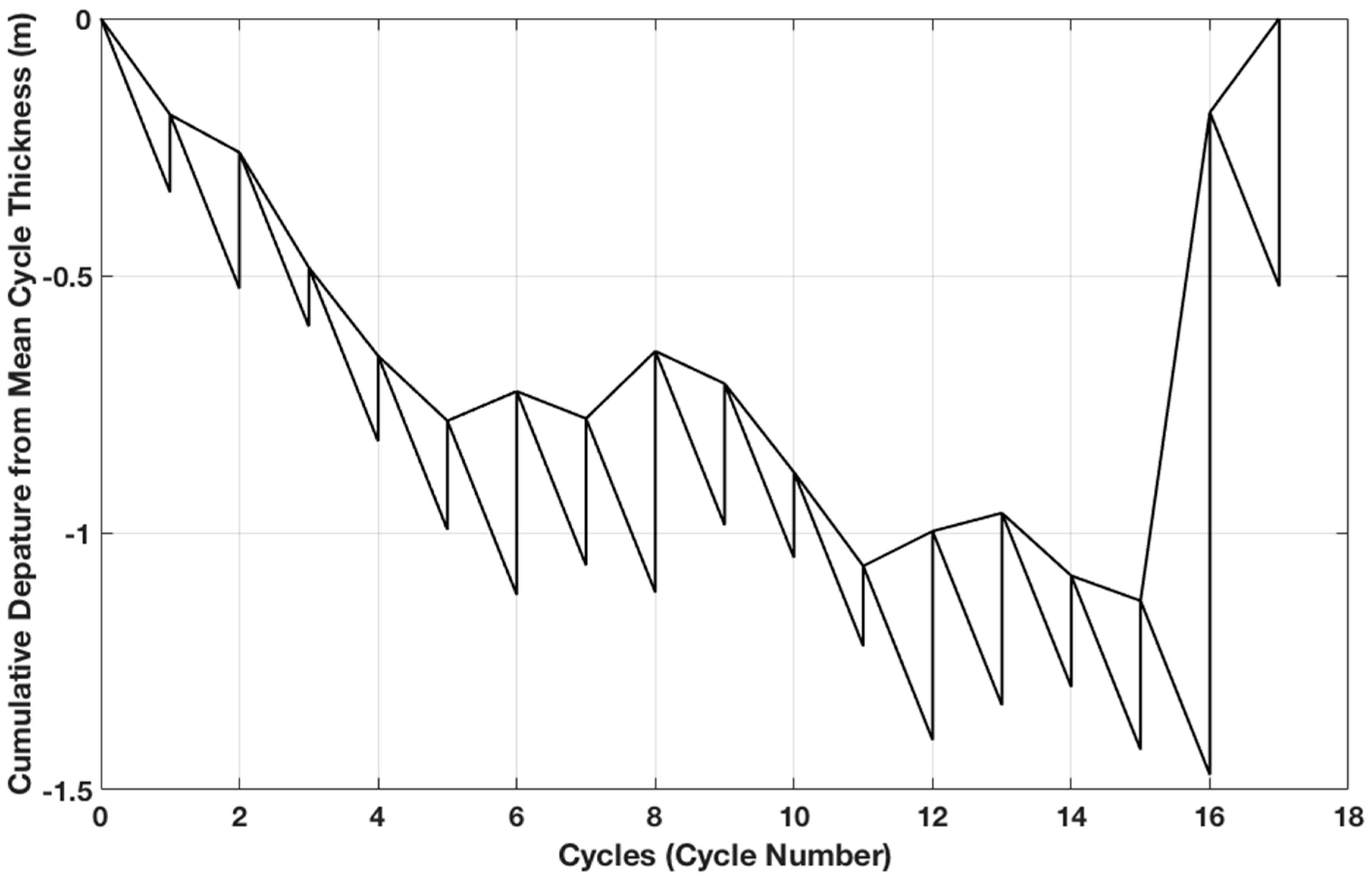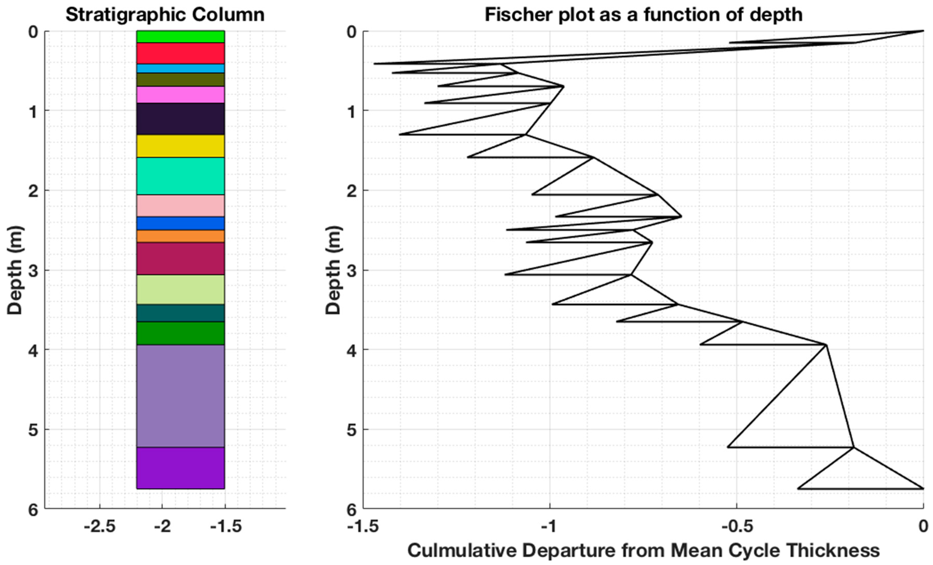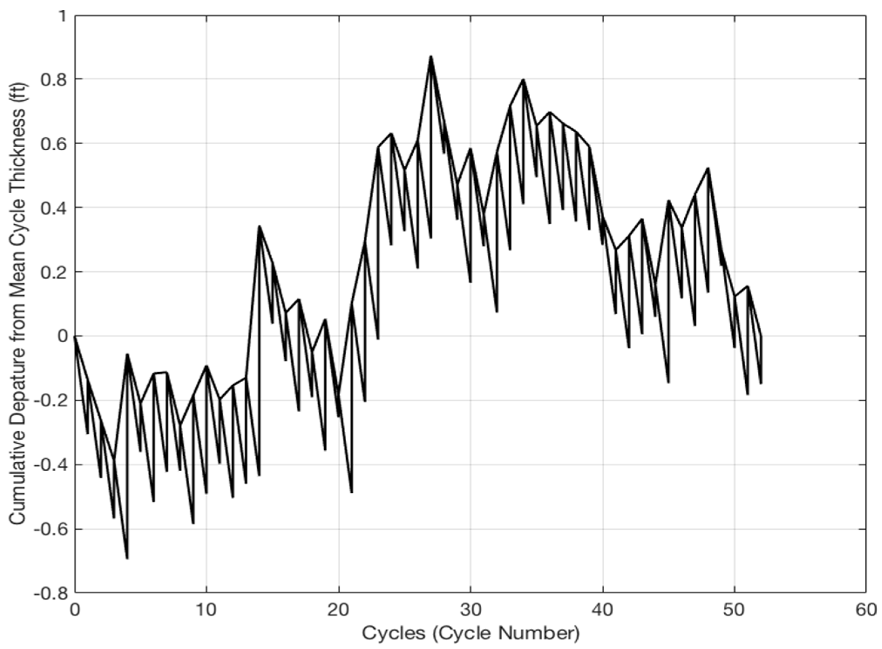Figure 3, Figure 4 and Figure 5 show the suite of Fischer plots and types generated by FischerLab. In Figure 3, Figure 4 and Figure 5, trends with a positive slope indicate an increase in accommodation, while trends with a negative slope indicate a decrease in accommodation. We also apply FischerLab to data from the Glen Rose Formation of Central Texas to illustrate the use of FischerLab on a carbonate outcrop section with more cycles (Figure 6). The Glen Rose is a shallow-water carbonate formation deposited on the southeastward flank of the Llano Uplift. During the Lower Cretaceous, the area was located on a broad, shallow, marine, carbonate-dominated shelf, which was part of a larger carbonate-evaporite system that engulfed the Gulf of Mexico [23]. Sediments of the Llano uplift were exposed as islands [23]. High energy and supratidal conditions were maintained on these islands through Albian time [24]. The Glen Rose carbonates are fine-grained foraminifera wackestone to packstone. They contain a vertically repetitive succession of burrowed and laminated units [24].

4.2. Application to Wireline Well-Logs

FischerLab has been applied to gamma-ray and resistivity wireline logs from a carbonate platform in the Western Great Bahama Bank collected by Ocean Drilling Program (ODP) Leg 166, site 1003 [25]. The Great Bahama Bank (GBB) is the largest shallow-water carbonate platform of the Bahamian archipelago, which consists of several carbonate platforms [26,27,28]. The platform growth occurred in pulses during sea-level highstands bounded by unconformities, which were generated during sea-level lowstands [29]. The configuration of GBB as a flat-topped platform during Late Pliocene and Quaternary times [27,28] influenced the export pattern of shallow-water carbonate particles, which were produced on the bank top, and which supplied the slope of the bank [29]. Eberli and Ginsburg [27,28] studied the internal architecture of the platform using seismic data, and demonstrated that the modern platforms and channels of the GBB evolved in response to numerous cycles of erosional and progradational sedimentation overlaid upon an initial platform structure. The Western Great Bahama Bank predominantly consists of carbonates and local intercalations of evaporites [30]. Betzler et al. [29] studied the sedimentation patterns and turbidite frequency of the platform, and proposed that it was a depositional system that sheds calciturbidites during both highstands and lowstands of the sea level. Westphal et al. [31] documented the alternation of cemented and uncemented layers in the platform, and related their origin to differential shallow-burial diagenesis, rather than primary sediment composition.

Several studies observed the cyclic facies in the Bahama Bank [32,33]. Sediments recovered during ODP Leg 166 coring contain an excellent record of cyclic facies [25]. These cycles were apparent in the following logs: color reflectance, bulk density, p-wave velocity, natural gamma, and porosity data [32], and in the deep resistivity log. The fifth-order cycles were visually obvious as marked light- and dark-colored sediment alternations that were clearly recorded in the petrophysical measurements [32,33]. The fifth-order cycles are well correlated with the precessional orbital cyclicity linked to sea-level variations in many other Neogene successions [34]. The well-log data used in this study is from site 1003 of leg 166. Site 1003 was drilled in 483 m of water on the middle slope of the GBB, four kilometers from the platform’s edge [32]. The site penetrated 1300 m of mixed pelagic and bank-derived Neogene sediment, and the sediments had calcium carbonate contents generally between 60% and 97% [32]. Williams and Pirmez [33] derived the sedimentation rate from the cycle thicknesses in wireline well-logs from site 1003). At site 1003, apart from the gamma-ray (gAPI) and deep resistivity log (ohm), the other logs that show a cyclic signature are the uranium log (ppm) and the sonic velocity log (km/s). We chose the gamma-ray log and the resistivity log because they are available in many data sets. Other logs types may be used if they are observed to capture the cyclic variation of the carbonate platform facies. 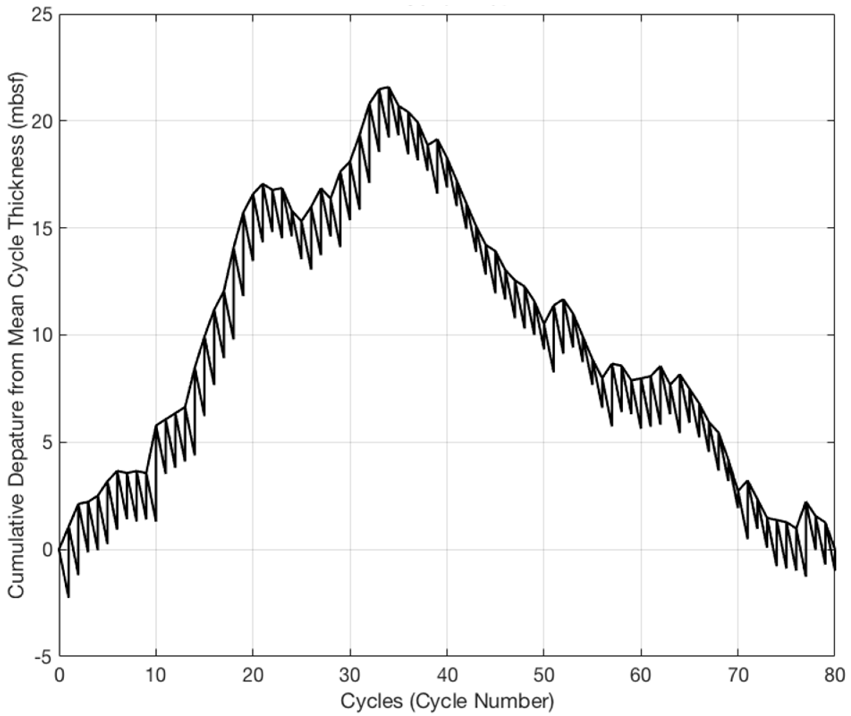Figure 7, Figure 8 and Figure 9 show the full suite of Fischer diagrams derived from the wireline log data obtained from the Bahamas (ODP Leg 166, Site 1003). In Figure 7, Figure 8 and Figure 9, trends with positive or negative slopes indicate increases and decreases in accommodation, respectively.

5. Conclusions

We developed FischerLab, a new program for the plotting and analysis of Fischer plots. FischerLab offers several significant improvements over the existing software. The program has an interactive graphical user interface that is easy to use. It was written in MATLAB and is distributed as a source code, which enables easy cross-platform portability. The source code can also be compiled into a stand-alone program. The program supports multiple data input formats, including CSV format, XSLX spreadsheet format, ASCII text format, and LAS format (the standard well-log information file format in the oil and gas, and water well industries). The program also supports several output formats, including PNG, FIG, GIF, and AVI formats.

Fischer plots are often applied to the stratigraphic data interpreted from exposed carbonate successions. In addition to accepting the traditional interpreted stratigraphic input, FischerLab gives geoscientists the flexibility to construct Fischer plots directly from wireline well-logs. This feature enables comparative sedimentology studies of subsurface carbonate successions and modern carbonate platforms.

We also introduced the concept of dynamic Fischer plots. Dynamic Fischer plots depict the transition of the Fischer plot in the cycle domain, together with the transition of the stratigraphic section in a relative depth domain. The dynamic plot facilitates the correlation of specific stratigraphic packages to parts of the accommodation cycle while simultaneously depicting the subsidence.

References

- Fischer, A.G. The lofer cyclothem of the Alpine Triassic. In Symposium on Cyclic Sedimentation; Kansas State Geological Survey Bulletin: Lawrence, KS, USA, 1964; Volume 169, pp. 107–149. [Google Scholar]
- Sadler, P.M.; Osleger, D.A.; Montanez, I.P. On the labeling, length, and objective basis of Fischer plots. J. Sediment. Res. 1993, 63, 360–368. [Google Scholar]
- Day, P.I. The Fischer diagram in the depth domain; a tool for sequence stratigraphy. J. Sediment. Res. 1997, 67, 982–984. [Google Scholar] [CrossRef]
- Burgess, P.M.; Wright, V.P.; Emery, D. Numerical forward modelling of peritidal carbonate parasequence development: Implications for outcrop interpretation. Basin Res. 2001, 13, 1–16. [Google Scholar] [CrossRef]
- Hardie, L.A.; Shinn, E.A. Carbonate Depositional Environments: Modern and Ancient. III: Tidal Flats; Colorado School of Mines Quarterly: Golden, CO, USA, 1986; Volume 81. [Google Scholar]
- Goldhammer, R.K.; Dunn, P.A.; Hardie, L.A. Depositional cycles, composite sea-level changes, cycle stacking patterns, and the hierarchy of stratigraphic forcing: Examples from Alpine Triassic platform carbonates. Geol. Soc. Am. Bull. 1990, 102, 535–562. [Google Scholar]
- Read, J.F.; Koerschner, W.F.; Osleger, D.A.; Bollinger, G.A.; Coruh, C. Field and modelling studies of Cambrian carbonate cycles, Virginia appalachians; Reply. J. Sediment. Res. 1991, 61, 647–652. [Google Scholar]
- Drummond, C.N.; Wilkinson, B.H. Carbonate cycle stacking patterns and hierarchies of orbitally forced eustatic sealevel change. J. Sediment. Res. 1993, 63, 369–377. [Google Scholar]
- Wilkinson, B.H.; Drummond, C.N.; Diedrich, N.W.; Rothman, E.D. Poisson processes of carbonate accumulation on Paleozoic and Holocene platforms. J. Sediment. Res. 1999, 69, 338–350. [Google Scholar]
- Drummond, C.N.; Dugan, P.J. Self-organizing models of shallow-water carbonate accumulation. J. Sediment. Res. 1999, 69, 939–946. [Google Scholar] [CrossRef]
- Overstreet, R.B.; Oboh-Ikuenobe, F.E.; Gregg, J.M. Sequence stratigraphy and depositional facies of lower Ordovician cyclic carbonate rocks, southern Missouri, USA. J. Sediment. Res. 2003, 73, 421–433. [Google Scholar]
- Read, J.F.; Sriram, S. A computer program for construction of Fischer plots. Compass 1990, 66, 73–78. [Google Scholar]
- Husinec, A.; Basch, D.; Rose, B.; Read, J.F. FISCHERPLOTS: An Excel spreadsheet for computing Fischer plots of accommodation change in cyclic carbonate successions in both the time and depth domains. Comput. Geosci. 2008, 34, 269–277. [Google Scholar] [CrossRef]
- Goldhammer, R.K.; Dunn, P.A.; Hardie, L.A. High frequency glacio-eustatic sealevel oscillations with Milankovitch characteristics recorded in Middle Triassic platform carbonates in northern Italy. Am. J. Sci. 1987, 287, 853–892. [Google Scholar] [CrossRef]
- Amosu, A.; Sun, Y. WheelerLab: An interactive program for sequence stratigraphic analysis of seismic sections, outcrops and well sections and the generation of chronostratigraphic sections and dynamic chronostratigraphic sections. SoftwareX 2017, 6, 19–24. [Google Scholar] [CrossRef]
- Amosu, A.; Sun, Y. WheelerLab: An Interactive Program for Sequence Stratigraphic Analysis of Seismic Sections and the Generation of Dynamic Chronostratigraphic Sections; Article 42053; American Association of Petroleum Geologists Search and Discovery: Tulsa, OK, USA, 2017; p. 3. [Google Scholar]
- Read, J.F.; Goldhammer, R.K. Use of Fischer plots to define third-order sea-level curves in Ordovician peritidal cyclic carbonates, Appalachians. Geology 1988, 16, 895–899. [Google Scholar] [CrossRef]
- Boss, S.K.; Rasmussen, K.A. Misuse of Fischer plots as sea-level curves. Geology 1995, 23, 221–224. [Google Scholar] [CrossRef]
- Amosu, A.; Sun, Y. Fischerlab: An interactive program for generating dynamic Fischer plots from wireline logs and stratigraphic data. In Proceedings of the AAPG Annual Convention and Exhibition, Houston, TX, USA, 2–5 April 2017. [Google Scholar]
- Imsalem, M. Preliminary establishment of Al-Athrun, Uwayliah and Apollonia formations based on magnetostratigraphic investigation, NE Libya. Master (i). Poitiers 2011. [Google Scholar] [CrossRef]
- Zert, B. Geological Map of Libya, 1: 250000. Sheet Dernah (N.I. 34–16). Explanatory Booklet; Industrial Research Centre: Tripoli, Libya, 1974; p. 49. [Google Scholar]
- Röhlich, P. Tectonic development of Al Jabal al Akhdar. In The Geology of Libya; Salem, M.J., Buserwil, M.T., Eds.; Academic Press: London, UK, 1980; Volume III, pp. 923–931. [Google Scholar]
- Kirkland, B.L.; Banner, J.L.; Moore, C.H.; Hoffman, C.; Pursell, B.; Vasquez, R. Cretaceous Cyclic Platform Carbonates of Central Texas; Prepared for: South Central Section Meeting of the Geological Society of America. Field trip #3: Austin; University of Texas: Austin, TX, USA, 1996; p. 36. [Google Scholar]
- Moore, C.H. A Field Guide to the Sequence-Stratigraphic Framework of Lower Cretaceous Platform Carbonates of Central Texas; Baton Rouge: Louisiana, CO, USA, 1995. [Google Scholar]
- Eberli, G.P.; Swart, P.K.; McNeill, D.F.; Kenter, J.A.M.; Anselmetti, F.S.; Melim, L.A.; Ginsburg, R.N. A synopsis of the Bahamas drilling project: Results from two deep core borings drilled on the Great Bahama Bank. In Proceedings of the Ocean Drilling Program, Initial Reports; Texas A&M University: College Station, TX, USA, 1997; Volume 166, pp. 23–41. [Google Scholar]
- Austin, J.A., Jr.; Schlager, W.; Palmer, A.A. Leg 101. Proceedings Initial Reports (Pt. A); Ocean Drilling Program: College Station, TX, USA, 1986. [Google Scholar]
- Eberli, G.P.; Ginsburg, R.N. Segmentation and coalescence of Cenozoic carbonate platforms, northwestern Great Bahama Bank. Geology 1987, 15, 75–79. [Google Scholar] [CrossRef]
- Eberli, G.P.; Ginsburg, R.N. Cenozoic Progradation of Northwestern Great Bahama Bank, a Record of Lateral Platform Growth and Sea-Level Fluctuations; The Society of Economic Paleontologists and Mineralogists (SEPM): Tulsa, OK, USA, 1989. [Google Scholar]
- Betzler, C.; Reijmer, J.J.; Bernet, K.; Eberli, G.P.; Anselmetti, F.S. Sedimentary patterns and geometries of the Bahamian outer carbonate ramp (Miocene–Lower Pliocene, Great Bahama Bank). Sedimentology 1999, 46, 1127–1143. [Google Scholar] [CrossRef]
- Meyerhoff, A.A.; Hatten, C.W. Bahamas salient of North America: Tectonic framework, stratigraphy, and petroleum potential. AAPG Bull. 1974, 58, 1201–1239. [Google Scholar]
- Westphal, H.; Head, M.J.; Munnecke, A. Differential diagenesis of rhythmic limestone alternations supported by palynological evidence. J. Sediment. Res. 2000, 70, 715–725. [Google Scholar] [CrossRef]
- Isern, A.R.; Anselmetti, F. The influence of carbonate platform morphology and sea level on fifth-order petrophysical cyclicity in slope and basin sediments adjacent to the great Bahama bank. Marine Geol. 2001, 177, 381–394. [Google Scholar] [CrossRef]
- Williams, T.; Pirmez, C. FMS images from carbonates of the Bahama bank slope, ODP Leg 166: Lithological identification and cyclo-stratigraphy. Geol. Soc. Spec. Publ. London 1999, 159, 227–238. [Google Scholar] [CrossRef]
- Shackleton, N.J.; Berger, A.; Peltier, W.R. An alternative astronomical calibration of the lower Pleistocene timescale based on ODP Site 677. Trans. R. Soc. Edinburgh Earth Sci. 1990, 81, 251–261. [Google Scholar] [CrossRef]
© 2020 by the authors. Licensee MDPI, Basel, Switzerland. This article is an open access article distributed under the terms and conditions of the Creative Commons Attribution (CC BY) license (http://creativecommons.org/licenses/by/4.0/).