Optimization of Technologies for Implementing Smart Metering in Residential Electricity Supplies in Peru

Abstract

This research evaluates the economic feasibility of implementing smart metering (SM) systems in Peruvian electricity distribution companies, prioritizing the maximization of the benefit–cost ratio (BCR). Seven communication architectures were analyzed in four companies, considering variables such as energy losses, meter costs, and per capita consumption. The results, evaluated through economic indicators such as the net present value, internal rate of return (IRR), and BCR showed that Luz Del Sur (LDS) obtained the best results, while ADINELSA (an electrical infrastructure management company), Sociedad Eléctrica Sur Oeste (SEAL), and Electro Sur Este (ELSE) presented the worst. The combination of power line communication and general packet radio service was the most viable architecture, followed by radio frequency mesh. However, this study concludes that a massive deployment of SM in Peru is not yet economically viable because of low per capita consumption and high meter costs. Future research should consider the benefits of distributed generation and demand management, as well as evaluate new communication technologies.

1. Introduction

The proposed model analyzes the impacts of SM, evaluating the improvements in technical losses and non-technical losses (NTLs), operating costs, and response to service interruptions.

According to [1] (p. 1), to meet the escalating energy needs of households, industries, and organizations, we require innovative solutions that promote responsible and economically sustainable consumption. Thus, the smart meter is the fundamental base for this process of innovation and development. The information provided by smart meters can be an invaluable and powerful tool for the planning of ESs [2].

Because information management is crucial, the authors of [3] explained that a smart grid benefits consumers by enabling a two-way flow of information between the utility and the customer. Similarly, the authors of [4] (pp. 2–3) stated that smart grids have a transformative impact on energy efficiency, offering significant benefits for users, distributors, and the environment. They help businesses balance supply with demand and avoid network congestion. They are resilient to fluctuations and disruptions because they can quickly detect and isolate problems and redirect energy flows.

According to [5] (pp. 19–20), the amount of SM within the countries of the European Union is expected to increase by 34% by the end of 2018 and up to 77% by 2024. In Peru, the most notable aspect has been the development of pilot projects in energy distribution companies (EDEs), involving a commitment to install 79,296 SM, with USD 17.6 million being invested (OSINERGMIN-Resolution fixing VAD 2028–2022 and 2019–2023 and its Annexes, 2018 and 2019) [6]. In this context, a simulation model is valuable for determining the best communication technological alternative for a specific ES when deploying the SM infrastructure (SMI) in Peru because of the initial investment costs and its technical complexity in terms of both communications and the particular characteristics of an ES.

The authors of [7] (p. 2) stated that the implementation of smart meters is revolutionizing traditional smart networks, promoting energy efficiency, and facilitating two-way communication between consumers and suppliers. Their study, “Exploring smart meters: what we know and what we need to know”, highlighted the importance of real-time information monitoring, accuracy, privacy, and security in the functionality of smart meters. The benefits align with improving customer awareness, energy efficiency, and network stability. The difficulties lie in privacy aspects and the limitations of current standards. The influential factors are cost–benefit analysis, regulatory policies, customer awareness, and technical considerations.

The disruptive challenges that service companies face have transformed the sector because of factors such as migration to cities, deregulation, the need for new infrastructure, changes in the workforce, and changes in demand, enabling service companies to reduce costs and increase income [8] (p. 1). Adding to this context is the growth of distributed generation (DG), with renewable energies (REs) as a generation source. Likewise, we have electric vehicles and their interconnection in electrical networks, with intelligent remote control and a change in the demand curve. These changes require the practical and real-time measurement of key parameters of equipment and sensors.

A study on the deployment of second-generation smart meters in Italy [9] (p. 1)] involved a cost–benefit analysis and highlighted Italy as a pioneer country in the deployment of smart meters, starting in 2000 and deploying 36.7 million meters between 2001 and 2011. The energy distribution companies recovered their investments via tariffs after some time, despite cost–benefit analysis being performed for them in particular.

To avoid the obsolescence of first-generation smart meters, which have a useful life of 15 years, and to add functionalities, a regulator designed a scheme for second-generation smart meters, starting the company E-Distribuzione, which has been deploying these meters since 2017. The decision to install this scheme without a cost–benefit analysis, unlike other countries of the European Union, was taken to avoid potential delays caused by an official cost–benefit analysis.

SM is a technology necessary for the development of smart networks and, in a broader context, smart cities. It primarily provides information that can be used to optimize the operation of ESs, including residential supplies.

Smart cities represent a critical opportunity to reduce energy consumption, combining demand services and improving network stability and quality of life [2] (p. 3). New generation energy systems leverage big data and digital technologies to collect and analyze data in real time and manage services more efficiently. These solutions are transforming the energy landscape, creating synergies to reduce emissions, improving efficiency, and increasing resilience.

The authors of [10] (p. ix) stated that analyzing the types of data generated by the SMI can enable the transformation of EDEs and generate efficiency measures on the demand and supply sides. Additionally, the great capacity for communication between the energy sector and consumers can establish strong relationships between suppliers and customers, a better understanding of needs and capabilities, and innovation opportunities.

Likewise, the authors of [3] (p. 6) emphasized the policy established by the United States (US), the Energy Independence and Security Act, which commissioned the National Institute of Standards and Technology (NIST) to develop a structure of protocols and standards that allow the interoperability of intelligent equipment and systems. It set objectives such as accelerating the identification and consensus of smart grid standards, establishing a robust smart grid interoperability panel, and creating testing and certification infrastructure.

The authors of [10] (p. 3) described the key aspects presented in Recommendations 2012/148/EU to support member states in their preparation and deployment of smart meters, including lessons learned and good practices established in about half of the member states. It provides guidelines for carrying out cost–benefit analysis to ensure that their respective evaluations are comparable, relevant, and based on comprehensive and realistic deployment plans. These recommendations consider ten common minimum functionalities that an intelligent metering system (i.e., SMI) needs, including for users.

The authors of [11] (p. 51) proposed an evaluation that goes beyond the cost–benefit analysis proposed by the European Union—a hybrid evaluation through multi-criteria––cost–benefit analysis (MC-CBA), which considers the impacts in heterogeneous areas, monetary and non-monetary impacts, the points of view of all stakeholders, and the management of input data with uncertainties.

In Latin America, identifying the reasons for the development of SM is especially relevant. In this vein, pilot projects have been executed based on existing measurement technologies for different geographical realities; a cost–benefit analysis is necessary to establish adequate legislation that, together with public policies, promotes the development of technologies adapted to reality and, thus, achieves the objectives, which are also scalable over time [12] (p. 130).

As mentioned in [9,10,11,12], the deployment of SM goes beyond the evaluation of benefits and costs and depends on state policies, regulatory development, and the involvement of all stakeholders, such as users, among other aspects. However, the positive impact of a massive deployment of SM is clear, as set out in [3,6,7].

The benefits of deploying an SMI, according to the reviewed literature, such as DG, demand management, and customers’ management of their own consumption, can be considered for future studies.

1.1. Research Contributions

The main contributions of this research are as follows:

• The development of a novel model to evaluate the optimal implementation of SM systems (SMSs) in Peru’s electrical distribution systems.
• The consideration of technological, geographical, consumption, and regulatory factors, identifying the most appropriate technologies and evaluating their impacts on a particular ES.
• A valuable tool for EDEs, regulatory and normative institutions, and the academic community enables the following:

  ○

  Informed decision-making by evaluating the technical and economic feasibility of different SMS implementation options.

  ○

  Optimized resources by identifying the optimal parameters for a massive deployment of SM.

  ○

  Improved energy efficiency by quantifying the potential benefits in terms of reducing technical losses, operating costs, and response times following interruptions.

  ○

  Contribution to the national energy policy by supporting the transition toward a more efficient and sustainable energy matrix.

This is pioneering research in Peru and aligns with the pilot projects of SMS implementation being carried out by the EDEs. The results obtained contribute to a better understanding of the challenges and opportunities associated with the adoption of this technology through a massive deployment in Peru.

1.2. Justification of the Methodology

The developed methodology is a unique approach to framing the problem, deploying communication technologies within an ES environment, with its own characteristics, from the points of view of its electrical infrastructure, the consumption patterns of its customers, and the regulatory framework specific to Peru, including tariffs, penalties for inadequate service quality, and technical and commercial losses. However, the NPV, IRR, and BCR are well-known economic parameters that allow for a quick, practical, and understandable comparison of the simulation results and various communication technologies, as well as that between the four companies being studied.

Thus, the present methodology proposes a unique approach to addressing SM deployment in Peru that is based on solid and widely disseminated knowledge, such as the NPV, IRR, and BCR, and the optimization of linear programming using the Excel SOLVER Microsoft Office Profesional Plus 2016.

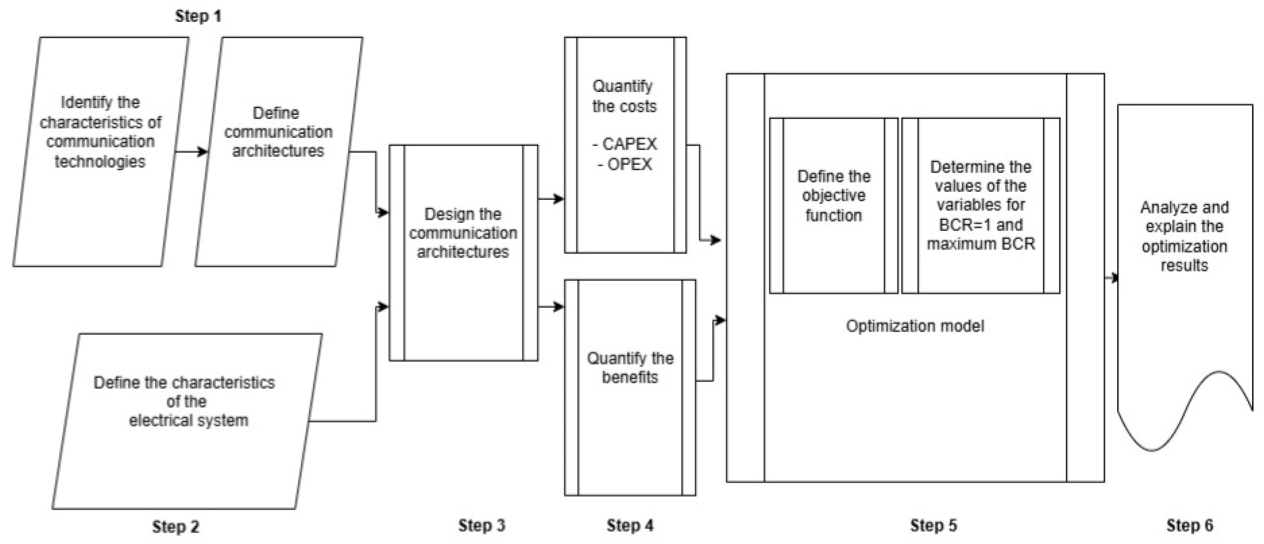
2. Materials and Methods

This section describes the procedure for modeling the intelligent measurement system as follows:

• The determination of communication technologies, architectures applicable to an SMI, and the characteristics of the ES.
• The determination of the relevant costs and benefits.
• The formulation of the model based on the design of metrics for each of the communication architectures and the calculation of economic indicators (NPV, IRR, and BCR).
• The optimization of variables (costs and benefits) for a viable SMI deployment (NPV ≥ 0; IRR ≥ 12%; BCR > 1).
• The simulation of the variables (costs and benefits) for a deployment of the SMI with BCR = 1.
• Simulation for the integration of cost variables (technical losses) for a viable SMI deployment.
• The analysis and discussion of the results for the indicators that reflect the viability of the SMI’s deployment.

The model allows simulations to be carried out for different communication technologies, as well as for variations in the main indicators under evaluation.

2.1. Characteristics of Communication Technologies

Wireless and wired systems are among the communication technologies with greater diffusion in recent years in SM.

Table 1. Communication technologies by author.

Technology/Source	[8]	[12]	[13]	[14]	Communication Type
Cellular (3G/4G/LTE)	√				Wireless
RF mesh	√				Wireless
PLC	√				Wired
PLC LF		√			Wired
PLC HF		√			Wired
RF LA		√			Wireless
RF mesh		√			Wireless
ZigBee			√		Wireless
GSM			√		Wireless
GPRS			√		Wireless
3G			√		Wireless
WiMAX			√		Wireless
Wi-Fi			√		Wireless
RF mesh				√	Wireless
Cellular (3G-4G)				√	Wireless
Cellular (GSM)				√	Wireless
Cellular (GPRS)				√	Wireless
ZigBee				√	Wireless
6LoWPAN				√	Wireless
Bluetooth				√	Wireless
Wi-Fi				√	Wireless
Enhanced Wi-Fi				√	Wireless
IEEE 802.11n				√	Wireless
WiMAX				√	Wireless
NB-PLC				√	Wired
BB-PLC				√	Wired
xDSL ADSL				√	Wired
xDSL HDSL				√	Wired
xDSL VHDSL				√	Wired
Euridis IEC 62056-31				√	Wired
PON				√	Wired

Note. RF, radio frequency mesh; LF, low frequency; HF, high frequency; GPRS, general packet radio service.

lists the wired technologies, which include broadband power line communication (PLC), narrowband PCL, digital subscriber line (DSL), and fiber optics.

Table 2. Communication technologies used by distribution companies.

Distribution Company	Country/Region	Communication Technology (Meters to Concentrator)	Communication (Concentrator to Control Center)	Communication Type
ONCOR	US/Texas	RF mesh and cellular	Cellular	Wireless
Commonwealth Edison	US/Illinois	RF mesh and cellular	Cellular	Wireless
Southern California Edison	US/California	RF mesh and cellular	Cellular	Wireless
Baltimore Gas & Electric	US/Maryland	RF mesh and cellular	Cellular and fiber optic	Hybrid
Electrobras Amazonas Energía	Brazil	RF mesh and cellular	Cellular	Wireless
ENEL	Italy	RF mesh, BPL, and cellular	PLC	Hybrid
PECO	US/Pennsylvania	Punto a punto via modem	Fiber optic	Hybrid
AusNet Service Company	Australia/Victoria	WiMax point to point	Fiber optic and cellular	Hybrid
CMS Energy	US/Michigan	Cellular	Cellular	Wireless
PEPCO	US/Washington DC	RF mesh	Cellular	Wireless
CESC Ltd.	India/Kolkata	RF mesh	Cellular and fiber optic	Hybrid
Tata Delhi Distribution Limited	India/Delhi	RF mesh and cellular	Fiber optic	Hybrid

lists the wireless technologies, which include low power, wide area networks (LPWANs), such as LoRaWAN, Sigfox, WiMAX, and cellular technologies.

The performance of communication technologies is generally determined by multiple factors for different applications, such as the consumption of the end equipment, the network size, and the transfer rate for up and down links [15] (p. 31).

The authors of [16] considered a set of criteria for evaluating the SMI, including the costs, security, scalability, interference, reliability, flexibility, privacy, speed of development, and access to development. However, because they did not evaluate specific communication technology brands, these are minimal criteria, and this study does not consider all of them.

This work used a bibliographic analysis to determine the characteristics of communication technologies. Table 1 presents descriptions of the communication technologies used in SMIs by different authors.

The authors of [17] present an advanced measurement infrastructure (AMI) architecture, which considers the information’s registration process, transmission, and further processing from the customer’s meter to the analysis reports.

Regarding communications, situations are the same in all countries because of the different technological levels and economic situations of the distribution operating companies [18] (p. 2). Challenges remain in applying these improvements to various countries. Many relate to the optimal communication architecture that allows for the adequate transfer of information in different conditions (urban, suburban, and rural) and the provision of the key requirements of availability, scalability, and reliability. However, a single solution does not exist because of the advantages and disadvantages of each possible communication protocol and different environmental aspects.

Depending on the most widespread communication technologies, distribution companies use the architectures detailed in Table 2. Thus, communication technologies vary between meter and concentrator, such as radio frequency (RF) mesh, long-range RF, cellular technology, and PLC. In the previous section, for concentrators and the control center, cellular technology, fiber optics, and PLC are considered.

Although using any communication system configuration, or architecture, is technically feasible, the choice is based on the costs of the equipment necessary to achieve reliable communications, the characteristics of the communication technology, such as its range, and ES’s characteristics.

Table 3. Segmented communication architectures.

Segmented		Architectures
Segment 1	Segment 2	Segment 1 + Segment 2
PLC	GPRS	PLC + GPRS
RF mesh	GPRS	RF mesh + GPRS
RF_LA	GPRS	RF_LA + GPRS
PLC	Fiber	PLC + fiber
RF mesh	Fiber	RF mesh + fiber
RF_LA	Fiber	RF_LA + fiber
RF_LA	RF LA	RF_LA + RF_LA

shows the different communication architectures.

The communication architecture in an AMI system is not limited to communication from the smart meters to the control center; this architecture extends to the clients and the EDE systems, as shown in Figure 1.

Despite the clear trend of innovation, the improvement in energy infrastructure is not uniform across different countries. Consequently, the use of smart meters worldwide varies. Even in countries with high technological development, ES operating companies are implementing updates for several reasons [18] (pp. 5, 16). The authors stated that, despite the different existing communication technologies, no one best solution exists. The optimal solution depends on many factors, including the current infrastructure, the geography, and the functionalities that the EDE wants to implement.

2.2. Characteristics of ESs

For the purposes of this study, ESs correspond to the distribution of low-voltage electrical energy, providing residential electrical supply. The physical infrastructure consists of the meters, which are housed in the meter holder box; the concentrators, which are housed in a distribution board; and the electrical networks (support structures, public lighting, electric cables, and distributed transformers, among other physical elements).

The experience of PEPCO, a service company in Washington DC, US, highlights the importance of conducting a survey of indoor meter boxes and basements to determine optimal locations for good communication for users and RF mesh systems [8] (p. 77).

However, ESs are developed in a geographical environment with unique characteristics, which may be flat or rugged, with or without buildings, with or without vegetation, and rainy or dry, i.e., lines between meters, concentrators, and the control center may not be visible.

For example, in the implementation of an AMI case by a service company in Kolkata, India, the RF signal of the communication network was interrupted by an iron bridge, which involved the installation of communication antennas in appropriate locations [9] (p. 40). Likewise, the service company ComEd in the US took measures to achieve a consistent network signal throughout the year, installing towers for the communication antennas to avoid interference from the seasonal foliage of trees and similar large blockages. However, the work required to prevent these interferences generates delays in the installation of AMI systems, which must be considered.

The authors of [12] (p. 26) stated that because of the physical interferences that occur over time (line-of-sight blockages), RF systems require significant maintenance. Likewise, they highlighted the importance of the communication system’s capacity to recover, for example, from system power failures, especially for RF mesh systems; poor service provision conditions can lead to such failures, producing service interruptions or ongoing maintenance needs. Added to this problem, for this same case of mesh topology, is the difficulty of detecting possible failures in the communication system due to the challenge of determining whether the failure corresponds to a blocked channel, a malfunction of the meter, or a bad connection.

Likewise, among the attributes of the ESs, we must consider the customer density and the length of the low-voltage feeders; for PLC technologies, a greater distance between the meter and concentrator reduces the reliability of communication because the physical means of the signals’ transport is exposed to the conditions of the network and the interferences inherent to the transmission of electricity.

The reliability of communication between the elements of smart networks is crucial for system operation. Communication networks are susceptible to electromagnetic interference generated by the complex environment of smart networks due to the increase in the use of power converter units. More converter use creates a higher level of electromagnetic interference, increasing the likelihood of exceeding the level of accumulated noise that the equipment can endure. The presence of semiconductor power equipment in the loads, such as lamps, chargers, and other non-linear charging equipment, is the main cause of the emissions produced [19] (p. 1). Sophisticated methods are needed to evaluate, first, the type of interference and, second, the effectiveness of the strategies to mitigate this interference [20] (p. 2).

The characteristics of the ESs are as follows:

• Number of single-phase and three-phase users;
• Number of distribution substations;
• Degree of interference;
• Width and length of the area (geography);
• Average LV (low voltage) circuit length;
• Degree of longitudinal uniformity.

2.3. Benefit–Cost Ratio Analysis

2.3.1. Benefit

Evaluating benefits is challenging because they and their beneficiaries are hard to identify, and they need to be defined as immediate, medium-term, or long-term. Benefits related to cost savings include reduced meter reading operating costs; reduced maintenance costs; lower or deferred costs for distribution capacity, transmission capacity, and generation capacity; fewer technical losses and NTLs; savings in electricity costs; reduced outage time; reduced CO₂ emissions; and reduced air pollution [21] (pp. 12–14). The authors of [22] listed the challenges that represent the technical losses, primarily due to Joule heating effects. NTLs refer to financial losses to the distribution system operator (DSO) [23].

To determine benefits, we propose a calculation method for both with- and without-project scenarios (baseline), complemented with a detailed description of the benefit and its calculation formula.

Benefits from the users’ perspective correspond to energy efficiency, where users can monitor their energy consumption, translating into savings on their utility bills [24] (pp. 44–47). Additionally, varying prices across the day allows them to shift their consumption to reduce their costs.

In addition, users can yield indirect benefits from cost savings for other market actors. According to the results of a study conducted by the European Commission (EC) among its 28 members, the most-mentioned benefits are operating savings, reductions in NTLs, and reductions in user bills due to improved energy efficiency. Finally, the article mentions other benefits of SM deployment, such as increased speed in commercial transactions and quick and efficient attention to consumer requests, but they are difficult to quantify.

Table 4. Primary advantages of implementing an SMI.

Benefit	[5]	[24]	[12]	Scoring
Reduction in billing due to energy efficiency	√		√	2
Meter reading and operational savings	√	√	√	3
Asset operation and maintenance	√			1
Deferral of distribution capacity	√			1
Reduction in technical losses	√			1
NTLs (administrative and fraud)	√	√	√	3
Outage management based on the societal value of lost load		√	√	2
Outage management based on reducing compensation		√		1
CO2 emissions reduction	√			1
Voltage monitoring		√	√	2

presents a summary of the benefits of an SMI proposed by various authors.

In summary, the direct and immediate benefits of deploying an SMI are fewer meter readings, the avoidance of service disconnections and reconnections due to non-payment, reductions in NTLs, and a decrease in the energy lost due to the rapid attention to service outages. However, additional benefits, depending on other factors (tariff policies and DG), can lead to demand management and, consequently, savings on investments in generation, transmission, and distribution infrastructure, aspects that are already part of smart grids, whose foundation is the deployment of SMIs.

Once the communication technology is selected, its beneficial features must be determined [21]. According to the Electric Power Research Institute (EPRI) methodology, a key aspect is the definition of the term “benefit” (of the smart grid project) as an impact that has value for the DSO, households, or society in general, and the benefit needs to be quantified. Additionally, quantified benefits need to be monetized so that they can be compared to other benefits. Finally, their paper [25] proposed the following basic formula for determining benefits:

$$B=C_{BL}-C_P$$

(1)

where B is the benefit, C_BL is the baseline cost, and C_P is the project cost.

Therefore, the following presents a detailed explanation of the considered benefits:

• Savings from reduced meter reading costs

Given that the cost corresponding to meter readings is avoided with the SMI, Equation (2) represents the direct value of the meter reading:

$$B_{A\_L}={Cl}_{LB}-{Cl}_P$$

(2)

where ${Cl}_{BL}$ and ${Cl}_{P }$ are the meter reading costs for the baseline and project, respectively.

2.

Savings from reduced disconnection and reconnection costs

To quantify the benefits associated with disconnections and reconnections, we require the percentage of customers who undergo these processes annually to estimate the savings obtained from the deployment of an AMI. Considering these factors, Equation (3) is proposed for determining the benefits of disconnections and reconnections:

$$B_{A\_C}=C_{CS\_LB}-C_{CS\_P}$$

(3)

where $C_{CS\_LB}$ and $C_{CS\_P}$ are the service disconnection costs for the baseline and project, respectively.

For the purposes of this study, disconnection costs are considered equivalent to reconnection costs, and therefore, we use a similar formula:

$$B_{A\_R}=C_{RS\_LB}-C_{RS\_P}$$

(4)

where $C_{RS\_LB}$ and $C_{RS\_P}$ are the reconnection costs for the baseline and project, respectively.

3.

Savings from reduced NTLs

The formula in Equation (5) used to calculate the benefits of reducing NTLs considers the reduction that can be achieved within meters. In the pre-project scenario, these losses are present, unlike in the post-project scenario. Thus, the formula is as follows:

$$B_{R_{PNT}}=\%PNT\times {\%PNT}_m\times {(N}_{m1}+N_{m3})\times C_{pf}\times C_e$$

(5)

where $\%PNT$ is the percent NTL, ${\%PNT}_m$ is the percent NTL at the meter, $N_{m1}$ is the number of single-phase meters, $N_{m3}$ is the number of three-phase meters, $C_{pf}$ is the final per capita consumption, and $C_e$ is the cost of energy sales.

4.

Savings from reduced unsupplied energy

For this study, aside from the multiple benefits of an AMI system, we consider the benefit of reduced unsupplied energy and savings from lower compensation payments due to the faster detection of outages. We do not expect an elimination of outages but, rather, a reduction in their number. Therefore, we assume a percentage reduction in outage hours and, consequently, unsupplied energy. The number of outage hours without the project corresponds to the pre-project scenario, while the reduction in outage hours corresponds to the post-project scenario, assuming a percentage decrease. These are shown in Equations (6) and (7):

$$B_{R_{ENS}}={ENS}_n\times \left(C_e-C_{mc}\right)$$

(6)

$${ENS}_n={\displaystyle \frac{C_{pf}\times 12\times D\times \%dS}{\left(8760-D\right)\times 100}}$$

(7)

where ENS_n is the net energy not supplied, D is the system average interruption duration index (SAIDI), %dS is the annual percentage SAIDI reduction, and C_mc is the average energy purchase cost.

5.

Savings from reduced outage compensation (Equations (8) and (9)) are as follows:

$$B_{R\_Comp}=e\times K\times {ENS}_n$$

(8)

$$K_i=\left[1+{\displaystyle \frac{N-N^{\prime }}{N^{\prime }}}+{\displaystyle \frac{D-D^{\prime }}{D^{\prime }}}\right]$$

(9)

where e is the unit compensation of 0.35 USD/kWh, K_i is the incidence rate, D’ is the annual SAIDI tolerance, N is the annual system average interruption frequency index (SAIFI), and N’ is the annual SAIFI tolerance.

Equation (9) follows the formulation established by [26]. As indicated in the Technical Quality Standard for Electrical Services (NTCSE), the second and third factors of the equation for K_i must be positive to be evaluated; if both are negative, the value of K_i is considered zero. Thus, in summary, the savings from compensation are as follows:

$$B=B_{R\_PNT}+B_{A\_L}+B_{A\_C}+B_{A\_R}+B_{R\_ENS}+B_{R\_Comp}$$

(10)

2.3.2. Costs

A fundamental aspect to consider when determining incurred costs is the comparison between the no-project scenario (i.e., without the SMI) and the with-project scenario (with the SMI), which includes all the associated costs. In this regard, the authors of [25] (p. 11) presented a non-exhaustive list of costs, which include reliability, environmental, energy security, and other costs, such as customer engagement programs and sunk costs associated with the installation of traditional meters. These costs can be broadly classified into two groups: investment costs (incurred at the beginning of the project) and operation and maintenance (O&M) costs.

• Initial investment costs (CAPEX). The most substantial investment cost is for the measuring instruments (MIs), followed by the data concentrators, whose costs vary based on technology. Labor costs finalize the initial capital expenditure.
• O&M costs (OPEX). Ongoing operational expenses encompass replacements for aging MIs and concentrators. However, higher costs typically involve software licenses for metering devices, software maintenance and updates, and communication charges, which depend on the chosen communication technology and are often billed by public utility telecommunication providers.

Based on the previous development, the costs to be evaluated are as follows:

$$C=C_I+C_{OM}$$

(11)

$$C_I=C_{MI}+C_C+C_S+C_{MO}$$

(12)

$$C_{OM}=C_{OM\_MI}+C_{OM\_C}+C_{OM\_S}+C_{OM\_∆PT}$$

(13)

where C is the total cost, C₁ is the investment cost, C_OM is the O&M cost, C_MI is the MI cost, C_C is the cost of the concentrator, C_S is the software cost, C_{OM_MI} is the O&M cost of MI, C_{OM_C} is the O&M cost of the concentrator, C_{OM_S} is the O&M cost of the software, and $C_{OM\_∆PT}$ is the technical loss of the variation in the cost of the O&M.

Table 5. Cost structure, equipment, and characteristics of the ES.

Costs	Equipment	ES
CAPEX	Capital Cost (Investment)
	Number of meters	Number of customers
	Number of concentrators	Number of SEDs
	Number of filters	Degree of interference
	Number of amplifiers	Network length
	Workforce	Number of customers/number of SEDs
OPEX	O&M costs
	Cellular communication costs	Number of SEDs
	Software licenses	Number of customers/SEDs/control center
	Software maintenance (update)	Number of customer/SEDs/control center

summarizes the costs in two large groups, CAPEX and OPEX.

2.4. SMI Modeling

2.4.1. Research Metamodel

The metamodel depicted in Figure 2 outlines the optimization process for selecting the most suitable architecture for a specific ES. Steps 1 and 2 involve defining the primary characteristics or criteria of communication technologies and ESs, respectively, which form the basis for designing the corresponding communication architecture. In Step 3, we design the communication architecture, and based on this, Step 4 determines the costs and benefits specific to the SMI, which are constrained by their respective magnitudes (e.g., the number of meters, number of substations, and technology costs). These serve as inputs for Step 5, which is divided into two sub-steps: modeling and performing economic indicator calculations. The subsequent step involves optimization to determine the indicator values that make the SMI deployment feasible, meaning that the economic indicators are greater than or equal to the required values for a viable SMI deployment. This is determined based on the BCR, which must be equal to or greater than unity.

The objective function is to maximize the BCR of the SMI, considering the performance of communication technologies and the characteristics of the ES, which primarily impact the costs and benefits of the SMI deployment infrastructure, both in the investment and O&M stages. Depending on the communication technology (PLC, RF mesh, or long-range RF), the characteristics of the ES, and its geographic environment, installing amplifiers and/or filters may be necessary for communication reliability, adding to the initial investment costs. Based on the amount of equipment, according to the ES and the communication technologies in its two segments (meter to concentrator and concentrator to control center), the total costs of each solution alternative are calculated based on the unit costs of each piece of equipment, installation, and O&M. Subsequently, the economic flow for costs is constructed and combined with benefits, allowing the calculation of economic indicators, such as the NPV, IRR, and BCR. Finally, these economic indicators are optimized based on cost and benefit parameters to determine the conditions under which the deployment of MIs is feasible.

2.4.2. Mathematical Model

For the formulation of the mathematical model, the following elements are described:

• Indices and sets

J—the set of architectures, $j=1, \dots , n_j$;

I—the set of components (smart meter, concentrator, and software) of the communication system, $i=1, \dots , n_i$;

K—the total investment costs (smart meter, concentrator, software and labor), $k=1, \dots , n_k$.

• Parameters

$C_{I_k}—\mathrm{t}\mathrm{h}\mathrm{e} \mathrm{i}\mathrm{n}\mathrm{v}\mathrm{e}\mathrm{s}\mathrm{t}\mathrm{m}\mathrm{e}\mathrm{n}\mathrm{t} \mathrm{c}\mathrm{o}\mathrm{s}\mathrm{t} \mathrm{o}\mathrm{f} \mathrm{t}\mathrm{h}\mathrm{e} \mathrm{c}\mathrm{o}\mathrm{m}\mathrm{p}\mathrm{o}\mathrm{n}\mathrm{e}\mathrm{n}\mathrm{t} k$;

$C_{{OM}_i}—\mathrm{t}\mathrm{h}\mathrm{e} \mathrm{o}\mathrm{p}\mathrm{e}\mathrm{r}\mathrm{a}\mathrm{t}\mathrm{i}\mathrm{o}\mathrm{n} \mathrm{a}\mathrm{n}\mathrm{d} \mathrm{m}\mathrm{a}\mathrm{i}\mathrm{n}\mathrm{t}\mathrm{e}\mathrm{n}\mathrm{a}\mathrm{n}\mathrm{c}\mathrm{e} \mathrm{c}\mathrm{o}\mathrm{s}\mathrm{t} \mathrm{o}\mathrm{f} \mathrm{t}\mathrm{h}\mathrm{e} \mathrm{c}\mathrm{o}\mathrm{m}\mathrm{p}\mathrm{o}\mathrm{n}\mathrm{e}\mathrm{n}\mathrm{t} i$;

$N_{m1}—\mathrm{t}\mathrm{h}\mathrm{e} \mathrm{n}\mathrm{u}\mathrm{m}\mathrm{b}\mathrm{e}\mathrm{r} \mathrm{o}\mathrm{f} \mathrm{s}\mathrm{i}\mathrm{n}\mathrm{g}\mathrm{l}\mathrm{e}\text{-}\mathrm{p}\mathrm{h}\mathrm{a}\mathrm{s}\mathrm{e} \mathrm{c}\mathrm{o}\mathrm{n}\mathrm{n}\mathrm{e}\mathrm{c}\mathrm{t}\mathrm{i}\mathrm{o}\mathrm{n}\mathrm{s}$;

$N_{m3}—\mathrm{t}\mathrm{h}\mathrm{e} \mathrm{n}\mathrm{u}\mathrm{m}\mathrm{b}\mathrm{e}\mathrm{r} \mathrm{o}\mathrm{f} \mathrm{t}\mathrm{h}\mathrm{r}\mathrm{e}\mathrm{e}\text{-}\mathrm{p}\mathrm{h}\mathrm{a}\mathrm{s}\mathrm{e} \mathrm{c}\mathrm{o}\mathrm{n}\mathrm{n}\mathrm{e}\mathrm{c}\mathrm{t}\mathrm{i}\mathrm{o}\mathrm{n}\mathrm{s}$;

$C_{cs}—\mathrm{t}\mathrm{h}\mathrm{e} \mathrm{s}\mathrm{e}\mathrm{r}\mathrm{v}\mathrm{i}\mathrm{c}\mathrm{e} \mathrm{d}\mathrm{i}\mathrm{s}\mathrm{c}\mathrm{o}\mathrm{n}\mathrm{n}\mathrm{e}\mathrm{c}\mathrm{t}\mathrm{i}\mathrm{o}\mathrm{n} \mathrm{c}\mathrm{o}\mathrm{s}\mathrm{t}$;

$C_{rs}—\mathrm{t}\mathrm{h}\mathrm{e} \mathrm{s}\mathrm{e}\mathrm{r}\mathrm{v}\mathrm{i}\mathrm{c}\mathrm{e} \mathrm{r}\mathrm{e}\mathrm{c}\mathrm{o}\mathrm{n}\mathrm{n}\mathrm{e}\mathrm{c}\mathrm{t}\mathrm{i}\mathrm{o}\mathrm{n} \mathrm{c}\mathrm{o}\mathrm{s}\mathrm{t}$;

$C_s—\mathrm{t}\mathrm{h}\mathrm{e} \% \mathrm{a}\mathrm{n}\mathrm{n}\mathrm{u}\mathrm{a}\mathrm{l} \mathrm{s}\mathrm{e}\mathrm{r}\mathrm{v}\mathrm{i}\mathrm{c}\mathrm{e} \mathrm{d}\mathrm{i}\mathrm{s}\mathrm{c}\mathrm{o}\mathrm{n}\mathrm{n}\mathrm{e}\mathrm{c}\mathrm{t}\mathrm{i}\mathrm{o}\mathrm{n}$;

$C_l—\mathrm{t}\mathrm{h}\mathrm{e} \mathrm{m}\mathrm{o}\mathrm{n}\mathrm{t}\mathrm{h}\mathrm{l}\mathrm{y} \mathrm{r}\mathrm{e}\mathrm{a}\mathrm{d}\mathrm{i}\mathrm{n}\mathrm{g} \mathrm{c}\mathrm{o}\mathrm{s}\mathrm{t}$;

$CFI—\mathrm{t}\mathrm{h}\mathrm{e} \% \mathrm{o}\mathrm{f} \mathrm{t}\mathrm{h}\mathrm{e} \mathrm{f}\mathrm{i}\mathrm{x}\mathrm{e}\mathrm{d} \mathrm{c}\mathrm{h}\mathrm{a}\mathrm{r}\mathrm{g}\mathrm{e} \mathrm{a}\mathrm{t}\mathrm{t}\mathrm{r}\mathrm{i}\mathrm{b}\mathrm{u}\mathrm{t}\mathrm{e}\mathrm{d} \mathrm{t}\mathrm{o} \mathrm{m}\mathrm{e}\mathrm{t}\mathrm{e}\mathrm{r} \mathrm{r}\mathrm{e}\mathrm{a}\mathrm{d}\mathrm{i}\mathrm{n}\mathrm{g}\mathrm{s}$;

$C_{mc}—\mathrm{t}\mathrm{h}\mathrm{e} \mathrm{a}\mathrm{v}\mathrm{e}\mathrm{r}\mathrm{a}\mathrm{g}\mathrm{e} \mathrm{e}\mathrm{n}\mathrm{e}\mathrm{r}\mathrm{g}\mathrm{y} \mathrm{p}\mathrm{u}\mathrm{r}\mathrm{c}\mathrm{h}\mathrm{a}\mathrm{s}\mathrm{e} \mathrm{c}\mathrm{o}\mathrm{s}\mathrm{t}$;

$C_{cens}—\mathrm{t}\mathrm{h}\mathrm{e} \mathrm{p}\mathrm{e}\mathrm{n}\mathrm{a}\mathrm{l}\mathrm{t}\mathrm{y} \mathrm{f}\mathrm{o}\mathrm{r} \mathrm{n}\mathrm{o}\mathrm{n}-\mathrm{s}\mathrm{u}\mathrm{p}\mathrm{p}\mathrm{l}\mathrm{i}\mathrm{e}\mathrm{d} \mathrm{e}\mathrm{n}\mathrm{e}\mathrm{r}\mathrm{g}\mathrm{y}$;

${\%PNT}_m—\mathrm{t}\mathrm{h}\mathrm{e} \mathrm{p}\mathrm{e}\mathrm{r}\mathrm{c}\mathrm{e}\mathrm{n}\mathrm{t}\mathrm{a}\mathrm{g}\mathrm{e} \mathrm{o}\mathrm{f} \mathrm{N}\mathrm{T}\mathrm{L}\mathrm{s} \mathrm{i}\mathrm{n} \mathrm{t}\mathrm{h}\mathrm{e} \mathrm{m}\mathrm{e}\mathrm{t}\mathrm{e}\mathrm{r}$;

$\%PT—\mathrm{t}\mathrm{h}\mathrm{e} \% \mathrm{o}\mathrm{f} \mathrm{t}\mathrm{e}\mathrm{c}\mathrm{h}\mathrm{n}\mathrm{i}\mathrm{c}\mathrm{a}\mathrm{l} \mathrm{l}\mathrm{o}\mathrm{s}\mathrm{s}\mathrm{e}\mathrm{s} \mathrm{i}\mathrm{n} \mathrm{L}\mathrm{V} (\mathrm{l}\mathrm{o}\mathrm{w}\text{-}\mathrm{v}\mathrm{o}\mathrm{l}\mathrm{t}\mathrm{a}\mathrm{g}\mathrm{e}) \mathrm{n}\mathrm{e}\mathrm{t}\mathrm{w}\mathrm{o}\mathrm{r}\mathrm{k}\mathrm{s}$;

${\%P}_e—\mathrm{t}\mathrm{h}\mathrm{e} \% \mathrm{o}\mathrm{f} \mathrm{t}\mathrm{o}\mathrm{t}\mathrm{a}\mathrm{l} \mathrm{l}\mathrm{o}\mathrm{s}\mathrm{s}\mathrm{e}\mathrm{s} \mathrm{i}\mathrm{n} \mathrm{L}\mathrm{V} \mathrm{n}\mathrm{e}\mathrm{t}\mathrm{w}\mathrm{o}\mathrm{r}\mathrm{k}\mathrm{s}$;

$D—\mathrm{t}\mathrm{h}\mathrm{e} \mathrm{S}\mathrm{A}\mathrm{I}\mathrm{D}\mathrm{I} \mathrm{r}\mathrm{e}\mathrm{a}\mathrm{l} (\mathrm{a}\mathrm{n}\mathrm{n}\mathrm{u}\mathrm{a}\mathrm{l})$;

$N—\mathrm{t}\mathrm{h}\mathrm{e} \mathrm{S}\mathrm{A}\mathrm{I}\mathrm{F}\mathrm{I} \mathrm{r}\mathrm{e}\mathrm{a}\mathrm{l} (\mathrm{a}\mathrm{n}\mathrm{n}\mathrm{u}\mathrm{a}\mathrm{l})$;

$D^{\prime }—\mathrm{t}\mathrm{h}\mathrm{e} \mathrm{S}\mathrm{A}\mathrm{I}\mathrm{D}\mathrm{I} \mathrm{t}\mathrm{o}\mathrm{l}\mathrm{e}\mathrm{r}\mathrm{a}\mathrm{n}\mathrm{c}\mathrm{e} \left(\mathrm{a}\mathrm{n}\mathrm{n}\mathrm{u}\mathrm{a}\mathrm{l}\right)$;

$N^{\prime }—\mathrm{t}\mathrm{h}\mathrm{e} \mathrm{S}\mathrm{A}\mathrm{I}\mathrm{F}\mathrm{I} \mathrm{t}\mathrm{o}\mathrm{l}\mathrm{e}\mathrm{r}\mathrm{a}\mathrm{n}\mathrm{c}\mathrm{e} (\mathrm{a}\mathrm{n}\mathrm{n}\mathrm{u}\mathrm{a}\mathrm{l})$;

$e—\mathrm{t}\mathrm{h}\mathrm{e} \mathrm{c}\mathrm{o}\mathrm{m}\mathrm{p}\mathrm{e}\mathrm{n}\mathrm{s}\mathrm{a}\mathrm{t}\mathrm{i}\mathrm{o}\mathrm{n} \mathrm{p}\mathrm{e}\mathrm{r} \mathrm{u}\mathrm{n}\mathrm{i}\mathrm{t}$;

${ENS}_n—\mathrm{t}\mathrm{h}\mathrm{e} \% \mathrm{o}\mathrm{f} \mathrm{t}\mathrm{o}\mathrm{t}\mathrm{a}\mathrm{l} \mathrm{l}\mathrm{o}\mathrm{s}\mathrm{s}\mathrm{e}\mathrm{s} \mathrm{i}\mathrm{n} \mathrm{L}\mathrm{V} \mathrm{n}\mathrm{e}\mathrm{t}\mathrm{w}\mathrm{o}\mathrm{r}\mathrm{k}\mathrm{s}$;

$Ki—\mathrm{t}\mathrm{h}\mathrm{e} \mathrm{i}\mathrm{m}\mathrm{p}\mathrm{a}\mathrm{c}\mathrm{t} \mathrm{f}\mathrm{a}\mathrm{c}\mathrm{t}\mathrm{o}\mathrm{r} \mathrm{o}\mathrm{f} \mathrm{t}\mathrm{h}\mathrm{e} \mathrm{S}\mathrm{A}\mathrm{I}\mathrm{D}\mathrm{I} \mathrm{a}\mathrm{n}\mathrm{d} \mathrm{S}\mathrm{A}\mathrm{I}\mathrm{F}\mathrm{I}$;

$\%dS—\mathrm{t}\mathrm{h}\mathrm{e} \mathrm{p}\mathrm{e}\mathrm{r}\mathrm{c}\mathrm{e}\mathrm{n}\mathrm{t} \mathrm{d}\mathrm{e}\mathrm{c}\mathrm{r}\mathrm{e}\mathrm{a}\mathrm{s}\mathrm{e} \mathrm{i}\mathrm{n} \mathrm{t}\mathrm{h}\mathrm{e} \mathrm{S}\mathrm{A}\mathrm{I}\mathrm{D}\mathrm{I};$

$F_C—\mathrm{t}\mathrm{h}\mathrm{e} \mathrm{l}\mathrm{o}\mathrm{a}\mathrm{d} \mathrm{f}\mathrm{a}\mathrm{c}\mathrm{t}\mathrm{o}\mathrm{r}$;

$F_p—\mathrm{t}\mathrm{h}\mathrm{e} \mathrm{l}\mathrm{o}\mathrm{s}\mathrm{s}\mathrm{e}\mathrm{s} \mathrm{f}\mathrm{a}\mathrm{c}\mathrm{t}\mathrm{o}\mathrm{r}$;

$N_{sed}—\mathrm{t}\mathrm{h}\mathrm{e} \mathrm{a}\mathrm{m}\mathrm{o}\mathrm{u}\mathrm{n}\mathrm{t} \mathrm{o}\mathrm{f} \mathrm{S}\mathrm{E}\mathrm{D}$;

$N_{if}—\mathrm{t}\mathrm{h}\mathrm{e} \mathrm{l}\mathrm{e}\mathrm{v}\mathrm{e}\mathrm{l} \mathrm{o}\mathrm{f} \mathrm{p}\mathrm{h}\mathrm{y}\mathrm{s}\mathrm{i}\mathrm{c}\mathrm{a}\mathrm{l} \mathrm{i}\mathrm{n}\mathrm{t}\mathrm{e}\mathrm{r}\mathrm{f}\mathrm{e}\mathrm{r}\mathrm{e}\mathrm{n}\mathrm{c}\mathrm{e}$;

$N_{ug}—\mathrm{t}\mathrm{h}\mathrm{e} \mathrm{l}\mathrm{e}\mathrm{v}\mathrm{e}\mathrm{l} \mathrm{o}\mathrm{f} \mathrm{g}\mathrm{e}\mathrm{o}\mathrm{g}\mathrm{r}\mathrm{a}\mathrm{p}\mathrm{h}\mathrm{i}\mathrm{c} \mathrm{u}\mathrm{n}\mathrm{i}\mathrm{f}\mathrm{o}\mathrm{r}\mathrm{m}\mathrm{i}\mathrm{t}\mathrm{y}$;

$L_m—\mathrm{t}\mathrm{h}\mathrm{e} \mathrm{a}\mathrm{v}\mathrm{e}\mathrm{r}\mathrm{a}\mathrm{g}\mathrm{e} \mathrm{c}\mathrm{i}\mathrm{r}\mathrm{c}\mathrm{u}\mathrm{i}\mathrm{t} \mathrm{l}\mathrm{e}\mathrm{n}\mathrm{g}\mathrm{t}\mathrm{h} \mathrm{o}\mathrm{f} \mathrm{L}\mathrm{V} \mathrm{b}\mathrm{y} \mathrm{S}\mathrm{E}\mathrm{D}$;

$L_a—\mathrm{t}\mathrm{h}\mathrm{e} \mathrm{a}\mathrm{n}\mathrm{t}\mathrm{e}\mathrm{n}\mathrm{n}\mathrm{a} \mathrm{r}\mathrm{a}\mathrm{n}\mathrm{g}\mathrm{e} (\mathrm{R}\mathrm{F}\_\mathrm{L}\mathrm{A})$;

$N_{ua}—\mathrm{t}\mathrm{h}\mathrm{e} \mathrm{n}\mathrm{u}\mathrm{m}\mathrm{b}\mathrm{e}\mathrm{r} \mathrm{o}\mathrm{f} \mathrm{u}\mathrm{s}\mathrm{e}\mathrm{r}\mathrm{s} \mathrm{p}\mathrm{e}\mathrm{r} \mathrm{a}\mathrm{n}\mathrm{t}\mathrm{e}\mathrm{n}\mathrm{n}\mathrm{a} (\mathrm{R}\mathrm{F}\_\mathrm{L}\mathrm{A})$;

${\%}_{rc}—\mathrm{t}\mathrm{h}\mathrm{e} \% \mathrm{o}\mathrm{f} \mathrm{m}\mathrm{e}\mathrm{t}\mathrm{e}\mathrm{r} \mathrm{b}\mathrm{o}\mathrm{x} \mathrm{r}\mathrm{e}\mathrm{p}\mathrm{l}\mathrm{a}\mathrm{c}\mathrm{e}\mathrm{m}\mathrm{e}\mathrm{n}\mathrm{t}\mathrm{s} (\mathrm{R}\mathrm{F}\_\mathrm{L}\mathrm{A})$;

$TC—\mathrm{t}\mathrm{h}\mathrm{e} \mathrm{e}\mathrm{x}\mathrm{c}\mathrm{h}\mathrm{a}\mathrm{n}\mathrm{g}\mathrm{e} \mathrm{r}\mathrm{a}\mathrm{t}\mathrm{e} \mathrm{f}\mathrm{r}\mathrm{o}\mathrm{m} \mathrm{P}\mathrm{E}\mathrm{N} \mathrm{t}\mathrm{o} \mathrm{U}\mathrm{S}\mathrm{D}$;

$i—\mathrm{t}\mathrm{h}\mathrm{e} 12\% \mathrm{d}\mathrm{i}\mathrm{s}\mathrm{c}\mathrm{o}\mathrm{u}\mathrm{n}\mathrm{t} \mathrm{r}\mathrm{a}\mathrm{t}\mathrm{e} \mathrm{f}\mathrm{o}\mathrm{r} \mathrm{t}\mathrm{h}\mathrm{e} \mathrm{P}\mathrm{e}\mathrm{r}\mathrm{u}\mathrm{v}\mathrm{i}\mathrm{a}\mathrm{n} \mathrm{e}\mathrm{l}\mathrm{e}\mathrm{c}\mathrm{t}\mathrm{r}\mathrm{i}\mathrm{c}\mathrm{i}\mathrm{t}\mathrm{y} \mathrm{m}\mathrm{a}\mathrm{r}\mathrm{k}\mathrm{e}\mathrm{t}$;

$B_{A\_L}—\mathrm{t}\mathrm{h}\mathrm{e} \mathrm{b}\mathrm{e}\mathrm{n}\mathrm{e}\mathrm{f}\mathrm{i}\mathrm{t}\mathrm{s} \mathrm{o}\mathrm{f} \mathrm{a}\mathrm{v}\mathrm{o}\mathrm{i}\mathrm{d}\mathrm{i}\mathrm{n}\mathrm{g} \mathrm{t}\mathrm{h}\mathrm{e} \mathrm{n}\mathrm{e}\mathrm{e}\mathrm{d} \mathrm{f}\mathrm{o}\mathrm{r} \mathrm{m}\mathrm{e}\mathrm{t}\mathrm{e}\mathrm{r} \mathrm{r}\mathrm{e}\mathrm{a}\mathrm{d}\mathrm{i}\mathrm{n}\mathrm{g}\mathrm{s}$;

$B_{A\_C}—\mathrm{t}\mathrm{h}\mathrm{e} \mathrm{b}\mathrm{e}\mathrm{n}\mathrm{e}\mathrm{f}\mathrm{i}\mathrm{t}\mathrm{s} \mathrm{o}\mathrm{f} \mathrm{a}\mathrm{v}\mathrm{o}\mathrm{i}\mathrm{d}\mathrm{i}\mathrm{n}\mathrm{g} \mathrm{s}\mathrm{e}\mathrm{r}\mathrm{v}\mathrm{i}\mathrm{c}\mathrm{e} \mathrm{i}\mathrm{n}\mathrm{t}\mathrm{e}\mathrm{r}\mathrm{r}\mathrm{u}\mathrm{p}\mathrm{t}\mathrm{i}\mathrm{o}\mathrm{n}\mathrm{s}$;

$B_{A\_R}—\mathrm{t}\mathrm{h}\mathrm{e} \mathrm{b}\mathrm{e}\mathrm{n}\mathrm{e}\mathrm{f}\mathrm{i}\mathrm{t}\mathrm{s} \mathrm{o}\mathrm{f} \mathrm{a}\mathrm{v}\mathrm{o}\mathrm{i}\mathrm{d}\mathrm{i}\mathrm{n}\mathrm{g} \mathrm{t}\mathrm{h}\mathrm{e} \mathrm{n}\mathrm{e}\mathrm{e}\mathrm{d} \mathrm{f}\mathrm{o}\mathrm{r} \mathrm{r}\mathrm{e}\mathrm{c}\mathrm{o}\mathrm{n}\mathrm{n}\mathrm{e}\mathrm{c}\mathrm{t}\mathrm{i}\mathrm{o}\mathrm{n}\mathrm{s}$.

• Decision variables

The variables that determine the value of the BCR are the benefits and costs. Thus, the benefits to be considered in the optimization process depend directly on per capita electricity consumption, such as the reductions in PM2.5, NOx emissions, and compensation. The costs are determined by the costs of the meters and the incidence of technical losses, given the variation in per capita consumption. Therefore, we have the following:

Direct variables

$C_{pi}—\mathrm{t}\mathrm{h}\mathrm{e} \mathrm{i}\mathrm{n}\mathrm{i}\mathrm{t}\mathrm{i}\mathrm{a}\mathrm{l} \mathrm{p}\mathrm{e}\mathrm{r} \mathrm{c}\mathrm{a}\mathrm{p}\mathrm{i}\mathrm{t}\mathrm{a} \mathrm{c}\mathrm{o}\mathrm{n}\mathrm{s}\mathrm{u}\mathrm{m}\mathrm{p}\mathrm{t}\mathrm{i}\mathrm{o}\mathrm{n}$;

$C_{pf}—\mathrm{t}\mathrm{h}\mathrm{e} \mathrm{f}\mathrm{i}\mathrm{n}\mathrm{a}\mathrm{l} \mathrm{p}\mathrm{e}\mathrm{r} \mathrm{c}\mathrm{a}\mathrm{p}\mathrm{i}\mathrm{t}\mathrm{a} \mathrm{c}\mathrm{o}\mathrm{n}\mathrm{s}\mathrm{u}\mathrm{m}\mathrm{p}\mathrm{t}\mathrm{i}\mathrm{o}\mathrm{n}$;

$C_{pm1}—\mathrm{t}\mathrm{h}\mathrm{e} \mathrm{c}\mathrm{o}\mathrm{s}\mathrm{t} \mathrm{o}\mathrm{f} \mathrm{a} \mathrm{s}\mathrm{i}\mathrm{n}\mathrm{g}\mathrm{l}\mathrm{e}\text{-}\mathrm{p}\mathrm{h}\mathrm{a}\mathrm{s}\mathrm{e} \mathrm{m}\mathrm{e}\mathrm{t}\mathrm{e}\mathrm{r} \mathrm{f}\mathrm{o}\mathrm{r} \mathrm{P}\mathrm{L}\mathrm{C}$;

$C_{pm3}—\mathrm{t}\mathrm{h}\mathrm{e} \mathrm{c}\mathrm{o}\mathrm{s}\mathrm{t} \mathrm{o}\mathrm{f} \mathrm{a} \mathrm{t}\mathrm{h}\mathrm{r}\mathrm{e}\mathrm{e}\text{-}\mathrm{p}\mathrm{h}\mathrm{a}\mathrm{s}\mathrm{e} \mathrm{m}\mathrm{e}\mathrm{t}\mathrm{e}\mathrm{r} \mathrm{f}\mathrm{o}\mathrm{r} \mathrm{P}\mathrm{L}\mathrm{C}$;

$C_{mm1}—\mathrm{t}\mathrm{h}\mathrm{e} \mathrm{c}\mathrm{o}\mathrm{s}\mathrm{t} \mathrm{o}\mathrm{f} \mathrm{a} \mathrm{s}\mathrm{i}\mathrm{n}\mathrm{g}\mathrm{l}\mathrm{e}\text{-}\mathrm{p}\mathrm{h}\mathrm{a}\mathrm{s}\mathrm{e} \mathrm{m}\mathrm{e}\mathrm{t}\mathrm{e}\mathrm{r} \mathrm{f}\mathrm{o}\mathrm{r} \mathrm{m}\mathrm{e}\mathrm{s}\mathrm{h}$;

$C_{mm3}—\mathrm{t}\mathrm{h}\mathrm{e} \mathrm{c}\mathrm{o}\mathrm{s}\mathrm{t} \mathrm{o}\mathrm{f} \mathrm{a} \mathrm{t}\mathrm{h}\mathrm{r}\mathrm{e}\mathrm{e}\text{-}\mathrm{p}\mathrm{h}\mathrm{a}\mathrm{s}\mathrm{e} \mathrm{m}\mathrm{e}\mathrm{t}\mathrm{e}\mathrm{r} \mathrm{f}\mathrm{o}\mathrm{r} \mathrm{m}\mathrm{e}\mathrm{s}\mathrm{h}$;

$C_{lm1}—\mathrm{t}\mathrm{h}\mathrm{e} \mathrm{c}\mathrm{o}\mathrm{s}\mathrm{t} \mathrm{o}\mathrm{f} \mathrm{a} \mathrm{s}\mathrm{i}\mathrm{n}\mathrm{g}\mathrm{l}\mathrm{e}\text{-}\mathrm{p}\mathrm{h}\mathrm{a}\mathrm{s}\mathrm{e} \mathrm{m}\mathrm{e}\mathrm{t}\mathrm{e}\mathrm{r} \mathrm{f}\mathrm{o}\mathrm{r} \mathrm{R}\mathrm{F}\_\mathrm{L}\mathrm{A}$;

$C_{lm3}—\mathrm{t}\mathrm{h}\mathrm{e} \mathrm{c}\mathrm{o}\mathrm{s}\mathrm{t} \mathrm{o}\mathrm{f} \mathrm{a} \mathrm{t}\mathrm{h}\mathrm{r}\mathrm{e}\mathrm{e}\text{-}\mathrm{p}\mathrm{h}\mathrm{a}\mathrm{s}\mathrm{e} \mathrm{m}\mathrm{e}\mathrm{t}\mathrm{e}\mathrm{r} \mathrm{f}\mathrm{o}\mathrm{r} \mathrm{R}\mathrm{F}\_\mathrm{L}\mathrm{A}$;

$\%PNT—\mathrm{t}\mathrm{h}\mathrm{e} \mathrm{p}\mathrm{e}\mathrm{r}\mathrm{c}\mathrm{e}\mathrm{n}\mathrm{t} \mathrm{o}\mathrm{f} \mathrm{N}\mathrm{T}\mathrm{L}\mathrm{s} \mathrm{a}\mathrm{t} \mathrm{L}\mathrm{V}$.

Indirect variables

$C_{∆PT}—\mathrm{t}\mathrm{h}\mathrm{e} \mathrm{e}\mathrm{n}\mathrm{e}\mathrm{r}\mathrm{g}\mathrm{y} \mathrm{l}\mathrm{o}\mathrm{s}\mathrm{s} \mathrm{d}\mathrm{u}\mathrm{e} \mathrm{t}\mathrm{o} \mathrm{t}\mathrm{h}\mathrm{e} \mathrm{i}\mathrm{n}\mathrm{c}\mathrm{r}\mathrm{e}\mathrm{a}\mathrm{s}\mathrm{e} \mathrm{i}\mathrm{n} \mathrm{p}\mathrm{e}\mathrm{r} \mathrm{c}\mathrm{a}\mathrm{p}\mathrm{i}\mathrm{t}\mathrm{a} \mathrm{c}\mathrm{o}\mathrm{n}\mathrm{s}\mathrm{u}\mathrm{m}\mathrm{p}\mathrm{t}\mathrm{i}\mathrm{o}\mathrm{n};$

$B_{R\_PNT}—\mathrm{t}\mathrm{h}\mathrm{e} \mathrm{b}\mathrm{e}\mathrm{n}\mathrm{e}\mathrm{f}\mathrm{i}\mathrm{t}\mathrm{s} \mathrm{o}\mathrm{f} \mathrm{N}\mathrm{T}\mathrm{L} \mathrm{a}\mathrm{c}\mathrm{c}\mathrm{o}\mathrm{r}\mathrm{d}\mathrm{i}\mathrm{n}\mathrm{g} \mathrm{t}\mathrm{o} \mathrm{t}\mathrm{h}\mathrm{e} \mathrm{p}\mathrm{e}\mathrm{r} \mathrm{c}\mathrm{a}\mathrm{p}\mathrm{i}\mathrm{t}\mathrm{a} \mathrm{c}\mathrm{o}\mathrm{n}\mathrm{s}\mathrm{u}\mathrm{m}\mathrm{p}\mathrm{t}\mathrm{i}\mathrm{o}\mathrm{n}$ C_p;

$B_{R\_ENS}—\mathrm{t}\mathrm{h}\mathrm{e} \mathrm{b}\mathrm{e}\mathrm{n}\mathrm{e}\mathrm{f}\mathrm{i}\mathrm{t}\mathrm{s} \mathrm{o}\mathrm{f} \mathrm{a}\mathrm{v}\mathrm{o}\mathrm{i}\mathrm{d}\mathrm{i}\mathrm{n}\mathrm{g} \mathrm{n}\mathrm{o}\mathrm{n}-\mathrm{s}\mathrm{u}\mathrm{p}\mathrm{p}\mathrm{l}\mathrm{i}\mathrm{e}\mathrm{d} \mathrm{e}\mathrm{n}\mathrm{e}\mathrm{r}\mathrm{g}\mathrm{y}, \mathrm{a}\mathrm{c}\mathrm{c}\mathrm{o}\mathrm{r}\mathrm{d}\mathrm{i}\mathrm{n}\mathrm{g} \mathrm{t}\mathrm{o}$ C_p;

$B_{R\_Comp}—\mathrm{t}\mathrm{h}\mathrm{e} \mathrm{b}\mathrm{e}\mathrm{n}\mathrm{e}\mathrm{f}\mathrm{i}\mathrm{t}\mathrm{s} \mathrm{d}\mathrm{u}\mathrm{e} \mathrm{t}\mathrm{o} \mathrm{a} \mathrm{r}\mathrm{e}\mathrm{d}\mathrm{u}\mathrm{c}\mathrm{t}\mathrm{i}\mathrm{o}\mathrm{n} \mathrm{i}\mathrm{n} \mathrm{c}\mathrm{o}\mathrm{m}\mathrm{p}\mathrm{e}\mathrm{n}\mathrm{s}\mathrm{a}\mathrm{t}\mathrm{i}\mathrm{o}\mathrm{n} \mathrm{f}\mathrm{o}\mathrm{r} \mathrm{i}\mathrm{n}\mathrm{t}\mathrm{e}\mathrm{r}\mathrm{r}\mathrm{u}\mathrm{p}\mathrm{t}\mathrm{i}\mathrm{o}\mathrm{n}\mathrm{s}$, $\mathrm{a}\mathrm{c}\mathrm{c}\mathrm{o}\mathrm{r}\mathrm{d}\mathrm{i}\mathrm{n}\mathrm{g} \mathrm{t}\mathrm{o}$ C_p.

• Objective function

The objective function involves maximizing the BCR (Equation (14)), which is achieved by maximizing profits and minimizing costs. Thus, the maximization function is applied to each of the communication architectures, from whose results the maximum value is obtained:

$$\mathrm{M}\mathrm{a}\mathrm{x}{\displaystyle \frac{B_{R_{PNT}}\left(f\left(C_{pf}\right)\right)+B_{R\_ENS}\left(f\left(C_{pf}\right)\right)+B_{R\_Comp}\left(f\left(C_{pf}\right)\right)+B_{A\_L}+B_{A\_C}+B_{A\_R}}{C_{MI}+∆PT \left(f\left(C_{pi}, C_{pf}\right)\right)}}$$

(14)

• Constraints

$C_{pi}=900 \mathrm{k}\mathrm{W}\mathrm{h}/\mathrm{m}\mathrm{o}\mathrm{n}\mathrm{t}\mathrm{h}$;

$C_{pf}=900 \mathrm{k}\mathrm{W}\mathrm{h}/\mathrm{m}\mathrm{o}\mathrm{n}\mathrm{t}\mathrm{h}$;

$C_{pm1}=34 \mathrm{U}\mathrm{S}\mathrm{D}/\mathrm{m}\mathrm{e}\mathrm{t}\mathrm{e}\mathrm{r}$;

$C_{pm3}=94 {\displaystyle \frac{\mathrm{U}\mathrm{S}\mathrm{D}}{\mathrm{m}\mathrm{e}\mathrm{t}\mathrm{e}\mathrm{r}}}$;

$C_{mm1}=44 \mathrm{U}\mathrm{S}\mathrm{D}/\mathrm{m}\mathrm{e}\mathrm{t}\mathrm{e}\mathrm{r}$;

$C_{mm3}=94 \mathrm{U}\mathrm{S}\mathrm{D}/\mathrm{m}\mathrm{e}\mathrm{t}\mathrm{e}\mathrm{r}$;

$C_{lm1}=82 \mathrm{U}\mathrm{S}\mathrm{D}/\mathrm{m}\mathrm{e}\mathrm{t}\mathrm{e}\mathrm{r}$;

$C_{lm3}=269 \mathrm{U}\mathrm{S}\mathrm{D}/\mathrm{m}\mathrm{e}\mathrm{t}\mathrm{e}\mathrm{r}$;

$\%PNT=5\%$;

$C_{pi}\le C_{pf}$.

In the modeling process, the initial and final per capita consumptions are considered variables, where the values that make the BCR are equal to one and the maximum values they can take.

2.4.3. Simulation Platforms

To carry out the simulations, we employed the Excel SOLVER platform, as shown in Figure 3, in which the objective function, constraints, and parameters were configured, and the BCR was maximized; a simulation was performed for BCR of 1, as developed in Section 2.4.1.

3. Results

The results of the optimization study show us two aspects: First, the technology with the best indicators among the seven alternatives; second, the highest BCRs among the four EDEs.

We present data on the ESs of four EDEs, including unit costs, per capita consumption, and tariffs. Then, we discuss the results for each EDE and analyze the key variables influencing these outcomes.

3.1. ES Characteristics

Table 6. Values for the parameters used for optimization (the quantities of supplies were obtained from the EDEs’ pilot projects (*) [6], the commercial data were taken from the EDEs’ websites and the geographic data are referential, determined by the authors).

Concept	Unit	LDS	SEAL	ADINELSA	ELSE
Supply
Single-phase supplies (Nm1)	Number	3152	7050	588	1662
Three-phase supplies (Nm3)	Number	163	485	6	678
Number of distribution substations (Nsed)	SED	22	54	3	9
Operational parameters
Service disconnection cost (Ccs)	PEN/month	7.22	6.45	12.08	7.29
Service reconnection cost (Crs)	PEN/month	10.03	8.68	15.26	9.7
Percent of service disconnections in year (% Cs)	%	10.00	10	10.00	10
Percent of reading participation fixed charge (% CFl)	%	19	18.17	18.17	18.17
Average energy purchase cost (Cmc)	PEN/kWh	0.32	0.38	0.36	0.37
Penalty for non-supplied energy (Cens)	USD/kWh	0.05	0.05	0.05	0.05
% reduction in NTLs on meter (%PNTm)	%	20	20	20	20
% technical losses on LV network (%PT)	%	2.5	4.5	3.16	4.56
Percent total losses on LV network (%Pe)	%	6.5	6.7	5.4	5.44
D (SAIDI base or actual)	Duration (hour)	9.73	21.74	7.89	8.22
D’ (SAIDI tolerance)	Duration	20	20	20	20
N (SAIFI base or actual)	Frequency (number of times)	2.67	5.95	1.50	3.81
N’ (SAIFI tolerance)	Frequency	12	12	12	12
Unit compensation e	USD/kWh	0.35	0.35	0.35	0.35
Percent decrease in SAIDI (%dS)	%	20	20	20	20
Load factor (Fc)		0.64	0.62	0.45	0.59
Losses factor (Fp)		0.47	0.46	0.28	0.42
Distribution substation
Physical interference (Nif)	Degrees	3	3	3	3
Geographic environment
Geographic uniformity (Nug)	Degrees	4	3	2	3
Average length of LV circuit per distribution substation (Lm)	m	150	150	150	150
Reach antenna + GPRS, RF LA (La)	km	3	3	3	3
Number of customers per antenna RF LA (Nua)	Unit	10,000	10,000	10,000	10,000
Percent meter box replacement (%rc)	%	10	10	10	10

(*) Submitted to OSINERGMIN as part of the tariff regulation process for electric distribution companies.

provides a comparative analysis of the characteristics of the ESs examined in this study. These systems belong to the four EDEs: Luz Del Sur (LDS), Sociedad Eléctrica del Sur Oeste (SEAL), ADINELSA (administrator of the state’s electrical infrastructure), and Electro Sur Este (ELSE). The simulation and optimization model was applied to these specific companies.

Table 7. Comparative characteristics of the four ESs examined in this study.

Criteria	LDS	SEAL	ADI	ELSE
Total number of enterprise customers	1,302,284	496,844	79,246	655,338
Service area	Lima south	Arequipa	Zona rural	Cusco
Annual sales volume GWh/año	8475	892	36	696
er capita consumption (kWh/month)	213.81	111.14	13.01	82.27
Type of management	Private	Public	Public	Public
Country/city	Perú	Perú	Perú	Perú

presents comparative indicators of the four companies analyzed in this article. It can be observed that the largest company is LDS, the smallest is ADINELSA, and SEAL and ELSE fall into intermediate sizes. The four companies are Peruvian, and only LDS belongs to the private sector.

Based on the costs incurred from the procurement process, a baseline equipment structure and corresponding unit costs were defined, as shown in

Table 8. Unit costs by components of the SMI (processed according to the information from the pilot projects) [6].

Supplies		Base Price (USD)
Meter
PLC
Single-phase meter (Cpm1)	Unit	67.69
Three-phase meter (Cpm3)	Unit	188.89
RF mesh
Single-phase meter (Cmm1)	Unit	88.88
Three-phase meter (Cmm3)	Unit	188.89
RF LA
Single-phase meter (Clm1)	Unit	164.97
Three-phase meter (Clm3)	Unit	538.49
Concentrator
PLC
Data collector (Ccd)	Unit	1817.59
Booster PLC (Crp)	Unit	1300.00
Filters (Cfp)	Unit	650.00
RF mesh
Data colector (Crm)	Unit	5836.07
RF Long Range
Collecting antenna (First and second section) (Cacl)	Unit	88,261.70
Collecting antenna + GPRS (Cacg)	Unit	88,261.70
Booster RF (Crr)	Unit	1300.00
Information Management Systems
Hardware
Servers	Unit
Software
Software of meter communication HES (head end system) (Csw)	Unit	13.16
Commercial application development (Cda)	Global
Custom application development (Cdc)	Global
Workforce
Initial investments
Customer communication (Cdif)	Unit
Network assessment situation (Cdig)	Global
Engineering and design (Cid)	Unit	11.39
Customer notification (Cnc)	Unit
Customer enabling (Chs)	Unit
Functional tests (Cps)	Unit
Training and development (Cec)	Global	2.89
Equipment installation
PLC
Single-phase meter installation (Cmp1)	Unit	15.83
Three-phase meter installation (Cmp3)	Unit	36.45
Data collector installation (Cmpc)	Unit	158.36
Booster installation PLC (Cmpr)	Unit	158.36
Filter installation (Cmf)	Unit	158.36
RF mesh
Single-phase meter installation (Cmm1)	Unit	16.00
Three-phase meter installation (Cmm3)	Unit	36.45
Data collector installation (Cmmc)	Unit	158.36
RF Largo Alcance
Single-phase meter installation (Cml1)	Unit	15.54
Three-phase meter installation (Cml3)	Unit	36.45
Change from metal junction box to polycarbonate (Clcc)	Unit	9.21
Installation of the data collection antenna (Cla)	Unit	316.71
Booster installation RF (Clr)	Unit	158.36
Second section implementation
Implementation of the MI control center GPRS (Cccg)	Global	10,000.00
Implementation of the MI control center RF LA (Cccl)	Global	88,261.70
Supply and installation of fiber optics (Cfo)	km	3500.00
O&M Costs
PLC
Service GPRS (annual) (Cpmg)	Unit	4.80
Software maintenance and updates HES (annual) (Cpms)	Unit	3.47
RF mesh
Service GPRS (annual) (Cmmg)	Unit	4.80
Software maintenance and updates HES (annual) (Cmms)	Unit	3.47
RF Largo Alcance
Service GPRS (annual) (Clms)	Unit	4.80
Software maintenance and updates HES (annual) (Clms)	Unit	3.47

:

Table 9. Per capita consumption and NTL by company (technical and commercial information published by OSINERGMIN) [27].

Concept	Unit	LDS	SEAL	ADINELSA	ELSE
Cp (per capita consumption)	kWh/month	213.81	111.14	13.01	82.27
%PNT	%	1.38	2.26	2.23	2.73

presents the average per capita consumption values for residential customers in the pilot project areas, along with the NTL levels at the distribution level.

The tariffs across different EDEs in Peru are similar, maintaining the same structure for three consumption tiers. Lower energy consumption tiers correspond to lower prices, while higher consumption tiers incur greater costs. This aspect is crucial for the present study, as the benefits of deploying SMI are calculated based on per capita consumption. The volume of consumption directly impacts the benefits derived from reducing NTLs and savings in compensation.

Table 10. Electricity rates by company (data obtained from the tariff sheets published by each company) [28,29,30,31].

Concept	Unit	LDS	SEAL	ADINELSA	ELSE
BT5B residential energy cost (Ce)	cent USD/kWh/month	14.92	13.65	24.33	14.66
0–30 kWh	cent USD/kWh/month	14.92	13.65	24.33	14.66
31–140 kWh	cent USD/kWh/month	21.32	19.50	60.83	20.94
>140 kWh	cent USD/kWh/month	22.06	20.01	62.77	21.61
Monthly fixed charge (CF)	USD/kWh/month	0.84	1.01	1.89	1.03

shows a summary of the rates.

3.2. Simulation Results

The analysis and calculations were conducted using a spreadsheet as an interface between the user and the model for data input, optimization, simulation, and result visualization. Initially, the analysis was performed using unoptimized and unsimulated data to understand the current reality. Subsequently, we conducted a simulation to determine the maximum BCRs, followed by a simulation to identify the variable values that resulted in a BCR of unity.

The results for each of the four companies are presented below.

3.2.1. LDS

Table 11. Current, constraint, and optimized costs for LDS.

Variable	Current ES Value (kWh/Month)	Constraint (kWh/Month)	Value for Max BCR (Ratio)	Value for BCR = 1
Cpi	213.81	900.0	900.0	610.1
Cpf	213.81	900.0	900.0	610.1
Cmi_plc1	67.69	34.0	34.0	37.5
Cmi_plc3	188.89	94.0	94.0	95.4
Cmi_mesh1	88.88	44.0	88.9	88.9
Cmi_mesh3	188.89	94.0	188.9	188.9
Cmi_rf1	164.97	82.0	165.0	165.0
Cmi_rf3	538.49	269.0	538.5	538.5
%PNT	1.38	5.0	5.0	3.4

shows that the baseline values of the variables undergo significant changes to achieve a BCR of one and make the deployment of an SMI feasible. Thus, per capita consumption must increase from 213.81 to 610.1 kWh/month, the cost of a single-phase meter must decrease from USD 67.69 to USD 37.5, that of a three-phase meter must decrease from USD 188.89 to USD 95.4, and the %PNT must increase from 1.38 to 3.4. Similarly, for optimization, the variables must equal the constraint values.

Table 12. Summary of results for LDS baseline case (without optimization).

Item	Architecture	Cost (USD)	NPV M (USD)	IRR	BCR
1	PLC + GPRS	471 M	−S/341	−5.7%	0.38
2	RF mesh + GPRS	604 M	−S/474	−8.2%	0.31
3	RF_LA + GPRS	865 M	−S/734	−11.4%	0.22
4	PLC + Fiber	482 M	−S/352	−5.9%	0.37
5	RF mesh + Fiber	616 M	−S/485	−8.3%	0.30
6	RF_LA + Fiber	876 M	−S/745	−11.5%	0.22
7	RF_LA + RF_LA	943 M	−S/813	−12.2%	0.20
				OF:	0.38

presents the results for the baseline scenario, i.e., without optimization, where the objective function (OF) is BCR = 0.38; SM deployment is not viable because this is less than unity. The technology with the best results is PLC + GPRS, closely followed by PLC + fiber.

Table 13. Summary of LDS optimization results for BCR = 1.

Item	Architecture	Cost (USD)	NPV (USD)	IRR	BCR
1	PLC + GPRS	360 M	−S/0	12.0%	1.00
2	RF mesh + GPRS	604 M	−S/244	3.6%	0.64
3	RF_LA + GPRS	865 M	−S/504	−1.0%	0.47
4	PLC + Fiber	372 M	−S/11	11.5%	0.98
5	RF mesh+ Fiber	616 M	−S/255	3.4%	0.63
6	RF_LA+ Fiber	876 M	−S/515	−1.2%	0.46
7	RF_LA + RF_LA	943 M	−S/582	−2.1%	0.43
				OF:	1.00

presents the results for the scenario with a BCR of 1, which shows a lower investment for the IRR of 12%, with PLC + GPRS as the best communication technology.

Table 14. Summary of LDS optimization results for maximum BCR.

Item	Architecture	Cost (USD)	NPV M (USD)	IRR	BCR
1	PLC + GPRS	349 M	S/322	27.5%	1.75
2	RF mesh + GPRS	604 M	S/67	14.0%	1.10
3	RF_LA + GPRS	865 M	−S/193	7.6%	0.79
4	PLC + Fiber	360 M	S/311	26.6%	1.71
5	RF mesh + Fiber	616 M	S/56	13.7%	1.08
6	RF_LA + Fiber	876 M	−S/204	7.4%	0.79
7	RF_LA + RF_LA	943 M	−S/272	6.2%	0.73
				OF:	1.75

presents the results for the scenario with the maximum BCR, which is 1.75 for the OF.

3.2.2. ADINELSA

Table 15. Current, constraint, and optimized costs for ADINELSA.

Variable	Current ES Values (kWh/Month)	Constraint (kWh/Month)	Value for Max BCR (Ratio)	Value for BCR = 1
Cpi	13.01	900.0	900.0	85.5
Cpf	13.01	900.0	900.0	85.5
Cmi_plc1	67.69	34.0	34.0	34.0
Cmi_plc3	188.89	94.0	94.0	94.0
Cmi_mesh1	88.88	44.0	88.9	88.9
Cmi_mesh3	188.89	94.0	188.9	188.9
Cmi_rf1	164.97	82.0	165.0	165.0
Cmi_rf3	538.49	269.0	538.5	538.5
%PNT	2.23	5.0	5.0	5.0

shows that the baseline values of the variables undergo significant changes to achieve a BCR of one. For instance, the per capita consumption must increase from 13.01 to 85.5 kWh/month, the cost of a single-phase meter must decrease from USD 67.69 to USD 34, the cost of a three-phase meter must decrease from USD 188.89 to USD 94, and the %PNT must increase from 2.23 to 5. Similarly, for optimization, the variables are equal to the constraint values.

Table 16. Summary of results for ADINELSA baseline case (without optimization).

Item	Architecture	Costs (USD)	NPV M (USD)	IRR	BCR
1	PLC + GPRS	86 M	−S/47	0.1%	0.53
2	RF mesh + GPRS	106 M	−S/66	−2.4%	0.45
3	RF_LA + GPRS	229 M	−S/190	−10.3%	0.22
4	PLC + fiber	87 M	−S/48	−0.1%	0.53
5	RF mesh + fiber	107 M	−S/68	−2.6%	0.44
6	RF_LA + fiber	240 M	−S/201	−10.7%	0.21
7	RF_LA + RF_LA	307 M	−S/268	−12.8%	0.17
				OF:	0.53

presents the results for the baseline scenario, i.e., without optimization, where the OF is BCR = 0.53; SM deployment is not viable because this is less than unity. The technologies with the best results are PLC + GPRS and PLC + fiber, followed by RF mesh + GPRS and RF mesh + fiber.

Table 17. Summary of ADINELSA optimization results for BCR = 1.

Item	Architecture	Cost (USD)	NPV M (USD)	IRR	BCR
1	PLC + GPRS	65 M	S/0	12.0%	1.00
2	RF mesh + GPRS	106 M	−S/40	4.2%	0.66
3	RF_LA + GPRS	229 M	−S/164	−5.3%	0.33
4	PLC+ Fiber	67 M	−S/1	11.6%	0.98
5	RF mesh + fiber	107 M	−S/42	4.0%	0.66
6	RF_LA+ fiber	240 M	−S/175	−5.8%	0.31
7	RF_LA + RF_LA	307 M	−S/242	−8.2%	0.25
				OF:	1.00

presents the results for the scenario with a BCR of 1, which show a lower investment for the IRR of 12%, with PLC + GPRS as the best communication technology.

Table 18. Summary of ADINELSA optimization results for the maximum BCR.

Item	Architecture	Cost (USD)	NPV M (USD)	IRR	BCR
1	PLC + GPRS	65 M	S/266	74.4%	4.35
2	RF mesh + GPRS	106 M	S/226	46.0%	2.89
3	RF_LA + GPRS	229 M	S/103	19.9%	1.42
4	PLC+ Fiber	67 M	S/265	72.7%	4.27
5	RF mesh+ Fiber	107 M	S/225	45.3%	2.85
6	RF_LA+ Fiber	240 M	S/92	18.7%	1.36
7	RF_LA + RF_LA	307 M	S/24	13.5%	1.08
				OF:	4.35

presents the results for the scenario for the maximum BCR, which is 4.35 for the OF.

3.2.3. SEAL

Table 19. Current, constraint, and optimized costs for SEAL.

Variable	Current ES Value (kWh/Month)	Constraint (kWh/Month)	Value for Max BCR (Ratio)	Value for BCR = 1
Cpi	111.14	900.0	900.0	460.0
Cpf	111.14	900.0	900.0	460.0
Cmi_plc1	67.69	34.0	34.0	34.0
Cmi_plc3	188.89	94.0	94.0	94.0
Cmi_mesh1	88.88	44.0	88.9	88.9
Cmi_mesh3	188.89	94.0	188.9	188.9
Cmi_rf1	164.97	82.0	165.0	165.0
Cmi_rf3	538.49	269.0	538.5	538.5
%PNT	2.26	5.0	5.0	5.0

shows that the baseline values of the variables undergo significant changes to achieve a BCR of one. The per capita consumption must increase from 111.14 to 460.0 kWh/month, the cost of a single-phase meter must decrease from USD 67.69 to USD 34, the cost of a three-phase meter must decrease from USD 188.89 to USD 94, and the %PNT must increase from 2.26 to 5. Similarly, for optimization, the variables are equal to the constraint values.

Table 20. Summary of results for SEAL baseline case (without optimization).

Item	Architecture	Costs (USD)	NPV M (USD)	IRR	BCR
1	PLC + GPRS	1087 M	−S/835	−7.4%	0.34
2	RF mesh + GPRS	1367 M	−S/1115	−9.6%	0.28
3	RF_LA + GPRS	1847 M	−S/1593	−12.2%	0.21
4	PLC + fiber	1115 M	−S/861	−7.6%	0.33
5	RF mesh + fiber	1396 M	−S/1141	−9.7%	0.27
6	RF_LA + fiber	1858 M	−S/1604	−12.2%	0.21
7	RF_LA + RF_LA	1926 M	−S/1671	−12.5%	0.21
				OF:	0.34

presents the results for the baseline scenario, i.e., without optimization, where the OF is BCR = 0.34; SM deployment is not viable because this is less than unity. The technologies with the best results are PLC + GPRS and PLC + fiber.

Table 21. Summary of SEAL optimization results for BCR = 1.

Item	Architecture	Cost (USD)	NPV M (USD)	IRR	BCR
1	PLC + GPRS	804 M	S/0	12.0%	1.00
2	RF mesh + GPRS	1367 M	−S/564	3.4%	0.64
3	RF_LA + GPRS	1847 M	−S/1042	−0.5%	0.49
4	PLC + fiber	832 M	−S/27	11.4%	0.97
5	RF mesh + fiber	1396 M	−S/590	3.2%	0.62
6	RF_LA + fiber	1858 M	−S/1053	−0.6%	0.48
7	RF_LA + RF_LA	1926 M	−S/1120	−1.0%	0.47
				OF:	1.00

presents the results for the scenario with a BCR of 1, which show a lower investment for the IRR of 12%. The best technologies are PLC + GPRS and PLC + fiber.

Table 22. Summary of SEAL optimization results for the maximum BCR.

Item	Architecture	Cost (USD)	NPV M (USD)	IRR	BCR
1	PLC + GPRS	804 M	S/592	24.5%	1.60
2	RF mesh + GPRS	1367 M	S/28	12.4%	1.02
3	RF_LA + GPRS	1847 M	−S/450	7.2%	0.78
4	PLC+ fiber	832 M	S/565	23.6%	1.56
5	RF mesh+ fiber	1396 M	S/1	12.0%	1.00
6	RF_LA+ fiber	1858 M	−S/461	7.1%	0.77
7	RF_LA + RF_LA	1926 M	−S/528	6.5%	0.75
				OF:	1.60

presents the results for the scenario for the maximum BCR, which is 1.60 for the OF.

3.2.4. ELSE

Table 23. Current, constraint, and optimized costs for ELSE.

Variable	Current ES Values (kWh/Month)	Constraint (kWh/Month)	Value for Max BCR (Ratio)	Value for BCR = 1
Cpi	82.27	900.0	900.0	461.5
Cpf	82.27	900.0	900.0	461.5
Cmi_plc1	67.69	34.0	34.0	34.0
Cmi_plc3	188.89	94.0	94.0	94.0
Cmi_mesh1	88.88	44.0	88.9	88.9
Cmi_mesh3	188.89	94.0	188.9	188.9
Cmi_rf1	164.97	82.0	165.0	165.0
Cmi_rf3	538.49	269.0	538.5	538.5
%PNT	2.73	5.0	5.0	5.0

shows that the baseline values of the variables undergo significant changes to achieve a BCR of one. The per capita consumption must increase from 82.271 to 461.5 kWh/month, the cost of a single-phase meter must decrease from USD 67.69 to USD 34, the cost of a three-phase meter must decrease from USD 188.89 to USD 94, and the %PNT must increase from 2.73 to 5. Similarly, for optimization, the variables must equal the constraint values.

Table 24. Summary of results for ELSE baseline case (without optimization).

Item	Architecture	Costs (USD)	NPV M (USD)	IRR	BCR
1	PLC + GPRS	391 M	−S/304	−7.8%	0.32
2	RF mesh + GPRS	448 M	−S/361	−9.1%	0.28
3	RF_LA + GPRS	853 M	−S/766	−14.6%	0.16
4	PLC + fiber	396 M	−S/308	−7.9%	0.32
5	RF mesh + Fiber	453 M	−S/366	−9.2%	0.28
6	RF_LA + Fiber	864 M	−S/777	−14.7%	0.16
7	RF_LA + RF_LA	931 M	−S/844	−15.3%	0.14
				OF:	0.32

presents the results for the baseline scenario, where the OF is BCR = 0.32; SM deployment is not viable because this is less than unity. The technologies with the same results are PLC + GPRS and PLC + fiber, followed by RF mesh + GPRS and RF mesh + Fiber.

Table 25. Summary of ELSE optimization results for BCR = 1.

Item	Architecture	Cost (USD)	NPV M (USD)	IRR	BCR
1	PLC + GPRS	271 M	−S/0	12.0%	1.00
2	RF mesh + GPRS	448 M	−S/177	3.8%	0.65
3	RF_LA + GPRS	853 M	−S/582	−4.2%	0.36
4	PLC+ fiber	276 M	−S/4	11.7%	0.99
5	RF mesh+ fiber	453 M	−S/182	3.7%	0.64
6	RF_LA+ fiber	864 M	−S/593	−4.3%	0.36
7	RF_LA + RF_LA	931 M	−S/660	−5.1%	0.33
				OF:	1.00

presents the results for the scenario with a BCR of 1, showing a lower investment for the IRR of 12%. The technologies that perform the best are PLC + GPRS and PLC + fiber.

Table 26. Summary of ELSE optimization results for the maximum BCR.

Item	Architecture	Cost (USD)	NPV M (USD)	IRR	BCR
1	PLC + GPRS	271 M	S/193	24.2%	1.59
2	RF mesh + GPRS	448 M	S/15	12.6%	1.03
3	RF_LA + GPRS	853 M	−S/389	2.4%	0.57
4	PLC+ fiber	276 M	S/188	23.7%	1.57
5	RF mesh+ fiber	453 M	S/11	12.5%	1.02
6	RF_LA+ fiber	864 M	−S/400	2.2%	0.56
7	RF_LA + RF_LA	931 M	−S/467	1.2%	0.53
				OF:	1.59

presents the results for the scenario for the maximum BCR, which is 1.59 for the OF.

In the present study, the optimization considered the fixed per capita consumption variable as an alternative that more closely approximates reality, given that a drastic increase in per capita consumption would not be expected over time. Thus,

Table 27. Maximum BCR for each architecture and EDE considering the per capita consumption variable as a fixed value.

Item/BCR	Architecture	LDS	SEAL	ADI	ELSE
1	PLC + GPRS	0.72	0.52	0.68	0.49
2	RF mesh + GPRS	0.45	0.33	0.45	0.31
3	RF_LA + GPRS	0.33	0.25	0.22	0.17
4	PLC + fiber	0.70	0.51	0.67	0.48
5	RF mesh + fiber	0.44	0.32	0.45	0.31
6	RF_LA + fiber	0.32	0.25	0.21	0.17
7	RF_LA + RF_LA	0.30	0.24	0.17	0.16

and Figure 4 show the optimization results for determining the maximum BCR for the four EDEs and the seven communication technologies. LDS has the highest BCR of 0.72, which is close to unity. This result is mainly explained by its higher per capita consumption, which is related to the PNT. In addition, ADINELSA’s maximum BCR is 0.68, which is close to the value of LDS, which is explained by the greater benefits from reducing commercial operating costs, such as the costs of meter readings, cuts, and reconnections, and their energy rates. Finally, SEAL and ELSE, with BCR values close to 0.50 and explained by their per capita consumptions, are less than 50% of that of LDS, and with values of their commercial parameters close to those of LDS.

Table 28. Maximum NPV for each architecture and EDE considering the per capita consumption variable as a fixed value.

Item/NPV	Architecture	LDS	SEAL	ADI	ELSE
1	PLC + GPRS	−S/121	−S/473	−S/25	−S/168
2	RF mesh + GPRS	−S/376	−S/1037	−S/66	−S/345
3	RF_LA + GPRS	−S/636	−S/1515	−S/189	−S/750
4	PLC + fiber	−S/131	−S/500	−S/27	−S/172
5	RF mesh + fiber	−S/386	−S/1063	−S/67	−S/350
6	RF_LA + fiber	−S/647	−S/1526	−S/200	−S/761
7	RF_LA + RF_LA	−S/714	−S/1593	−S/267	−S/828

and Figure 5 show that SEAL has the lowest NPV of -MS/1593 and the highest ADINELS of -MS/25. The reasons are the same as those that led to the BCR results.

Table 29. Maximum IRR for each architecture and EDE considering the per capita consumption variable as a fixed value.

Item/IRR	Architecture	LDS	SEAL	ADI	ELSE
1	PLC + GPRS	4.96%	−1.21%	3.99%	−2.1%
2	RF mesh + GPRS	−2.21%	−7.01%	−2.16%	−7.5%
3	RF_LA + GPRS	−6.09%	−9.83%	−10.07%	−13.3%
4	PLC + fiber	4.53%	−1.56%	3.70%	−2.3%
5	RF mesh + fiber	−2.39%	−7.16%	−2.30%	−7.6%
6	RF_LA + fiber	−6.22%	−9.89%	−10.49%	−13.4%
7	RF_LA + RF_LA	−6.96%	−10.21%	−12.64%	−14.0%

and Figure 6 show that LDS has the highest IRR of 4.96%, which is the closest to 12%, with the furthest being −14.0% for ELSE. In the same way, as for the BCR and NVP, the differences are explained by the per capita consumption levels for LDS, the lower investment levels for ADINELSA, and the intermediate results for ELSE and SEAL due to the intermediate values of these same variables.

4. Discussion

LDS shows the best performance for SM deployment, with BCR values of 0.72, close to unity, supported by the benefits of higher per capita consumption, which affect the reductions in NTLs and savings in commercial operating costs, such as those for meter readings and cuts and reconnections. However, ADINELSA, with a BCR of 0.68, also has good performance, given its high commercial operating costs and high rates, which, upon implementing an SMI, can become viable.

The technologies that show the best results are PLC and RF mesh, mainly because of their lower costs compared to long-range RF technology.

To achieve a BCR of unity for all cases, the optimization study shows the need for a significant reduction in meter costs, greater than 50%, but also a considerable increase in per capita consumption, which is unlikely in practice. In this same sense, the values obtained for optimization imply that the values of the variables reach the constraints.

As described in [32], the BCR can help define the limits of some parameters. In this line, the authors of [33] stated that the SM is a key component for meeting development demand, with the Internet of Things as a key technology.

5. Conclusions

An optimization model for an SMI was developed for residential supplies in Peru. This model allows for the determination of the optimal values for variables, making an SM deployment project viable according to the BCR OF.

The developed mathematical model considers OF as the maximization of the BCR, which is a function of the per capita consumption, meter costs, technical losses, and NTLs. SOLVER, excel complement software was used for the optimizations and simulations, due to its accessibility, ease of use, integration with the spreadsheet, and primarily because there is no need to obtain real-time results.

The model was applied to pilot projects for SM deployment in four EDEs—LDS, SEAL, ADINELSA, and ELSE. This allowed for the evaluation of the feasibility of smart meter deployment using the BCR, NPV, and IRR indicators. The best indicators were obtained for the LDS company (BCR = 0.72) and ADINELSA (BCR = 0.68), while the least promising indicators were obtained for SEAL (BCR = 0.52) and ELSE (BCR = 0.49), which achieved similar results because of their similar ES characteristics. Likewise, the communication architectures with the best indicators are PLC + GPRS and RF mesh + GPRS; the architecture with the lowest values corresponds to RF_LA because of the higher costs of the meters.

The developed model enabled the evaluation of the relationship between the characteristics of communication technologies and four ESs based on the results of the BCR, NPV, and IRR. We conclude that a massive deployment of SM in Peru is not viable, mainly because of the low per capita consumption in the residential sector and the high costs of SM systems.

References

1. Abdulrasheed, M.A.; Ahmed, M.S.; Abdullateef, A.A.; Oguntowo, B.I.; Aliyu, Y. Integrating IoT Systems for Real-Time Energy Monitoring and Efficiency in Smart Buildings. J. Mater. Environ. Sci. 2025, 16, 25–35. [Google Scholar]
2. Solis, R.; Gómez, G.A.; Saénz, K.J.; Ellis, A.J.; Navarro, W.J. Evaluación del comportamiento de la demanda en el modelado de las redes de distribución. Tecnol. Marcha 2025, 38, 115–127. [Google Scholar]
3. Nutakki, M.; Mandava, S. Review on optimization techniques and role of Artificial Intelligence in home energy management systems. Eng. Appl. Artif. Intell. 2023, 119, 105721. [Google Scholar] [CrossRef]
4. Michael, T.; Chukwudi, A.; Oluwajuwonlo, D.; Queen, Z. The impact of smart grid on energy efficiency: A comprehensive review. Eng. Sci. Technol. J. 2024, 5, 1257–1269. [Google Scholar] [CrossRef]
5. EC. Benchmarking Smart Metering Deployment in the EU-28: Final Report; European Commission: Brussels, Belgium, 2019; Available online: https://op.europa.eu/en/publication-detail/-/publication/b397ef73-698f-11ea-b735-01aa75ed71a1/language-en (accessed on 7 February 2025).
6. OSINERGMIN. Fijación del VAD 2022–2026 y 2023–2027. 2022. Available online: https://www.osinergmin.gob.pe/seccion/institucional/regulacion-tarifaria/procesos-regulatorios/electricidad/vad/fijacion-vad-2022-2026-y-2023-2027 (accessed on 7 February 2025).
7. Rajaguru, S.; Johansson, B.; Granath, M. Exploring Smart Meters: What We Know and What We Need to Know. In Perspectives in Business Informatics Research; Springer: Cham, Switzerland, 2023; Available online: https://link.springer.com/chapter/10.1007/978-3-031-43126-5_8 (accessed on 7 February 2025). [CrossRef]
8. World Bank Group. Survey of International Experience in Advanced Metering Infrastructure and Its Implementation; WBG: Washington, DC, USA, 2018; Available online: https://documentos.bancomundial.org/es/publication/documents-reports/documentdetail/957331569246407856/survey-of-international-experience-in-advanced-metering-infrastructure-and-its-implementation (accessed on 10 March 2025).
9. Stagnaro, C. Second-Generation Smart Meter Roll-Out in Italy: A Cost-Benefit Analysis. J. Ind. Bus. Econ. 2025, 52, 201–220. [Google Scholar] [CrossRef]
10. EC. Cost-Benefit Analyses & State of Play of Smart Metering Deployment in the EU-27; EC: Bruselas, Belgium, 2014; Available online: https://eur-lex.europa.eu/legal-content/EN/TXT/?uri=celex%3A52014SC0189 (accessed on 7 February 2025).
11. IEA-ISGAN. Annual Report 2018. Available online: https://www.iea-isgan.org/wp-content/uploads/2019/07/ISGAN-Annual-Report_2018_Web.pdf (accessed on 7 February 2025).
12. GTD. Estudio de Medidores Inteligentes y su Impacto en Tarifas; Comisión Nacional de Energía—CNE: Santiago de Chile, Chile, 2016; Available online: https://www.cne.cl/wp-content/uploads/2019/02/Informe-GTD-Medidores-Inteligentes-SMMC.pdf (accessed on 7 February 2025).
13. Quishpe, S.; Padilla, M.; Ruiz, M. Optimal Deployment of Wireless Networks for Smart Metering. Rev. Técnica Energía 2019, 16, 106–113. [Google Scholar]
14. Kochanski, M.; Korczak, K.; Skoczkowski, T. Technology Innovation System Analysis of Electricity Smart Metering in the European Union. Energies 2020, 13, 916. [Google Scholar] [CrossRef]
15. LoRaWan. A Technical Overview of LoRa® and LoRaWAN; LoRa Alliance: San Ramon, CA, USA, 2015; Available online: https://www.academia.edu/31617677/A_technical_overview_of_LoRa_and_LoRaWAN_What_is_it (accessed on 8 February 2025).
16. Abdul, D.; Wengi, J. Prioritization of renewable energy source for electricity generation through AHP-VIKOR integrated methodology. Sci. Direct 2022, 184, 1018–1032. [Google Scholar] [CrossRef]
17. Tangsunantham, N.; Chaiyod, P. Experimental Performance Analysis of Wi-SUN Channel Modelling Applied to Smart Grid Applications. Energies 2022, 15, 2417. [Google Scholar] [CrossRef]
18. Battista, G.; Marchesse, M.; Moheddine, A.; Patrone, F. A Possible Smart Metering System Evolution for Rural and Remote Areas Employing Unmanned Aerial Vehicles and Internet of Things in Smart Grids. Sensors 2021, 21, 1627. [Google Scholar] [CrossRef] [PubMed]
19. El Sayed, W. Electromagnetic Interference of Spread-Spectrum Modulated Power Converters in G3-PLC Power Line Communication Systems. IEEE Lett. EMC Pract. Appl. 2020, 3, 118–122. [Google Scholar] [CrossRef]
20. Llano, A.; Angulo, I.; Vega, D.; Marron, L. Virtual PLC Lab Enabled Physical Layer Improvement Proposals for PRIME and G3-PLC Standards. Appl. Sci. 2020, 10, 1777. [Google Scholar] [CrossRef]
21. ISGAN. Benefit & Cost Analyses and Toolkits. ISGAN Project. Annex 3; Ajou University: Suwon, Republic of Korea, 2015; Available online: https://www.iea-isgan.org/benefit-cost-analyses-and-toolkits/ (accessed on 7 February 2025).
22. Puma, D.W.; Molina, Y.P.; Atoccsa, B.A.; Luyo, J.E.; Naupari, Z. Distribution Network Reconfiguration Optimization Using a New Algorithm Hyperbolic Tangent Particle Swarm Optimization (HT-PSO). Energies 2024, 17, 3798. [Google Scholar] [CrossRef]
23. Badr, M.M.; Ibrahem, M.I.; Kholidy, H.A.; Fouda, M.M.; Ismail, M. Review of the Data-Driven Methods for Electricity Fraud Detection in Smart Metering Systems. Energies 2023, 16, 2852. [Google Scholar] [CrossRef]
24. DOE. Advanced Metering Infrastructure and Customer Systems. Results from the Smart Grid Investment Grant Program; US Department of Energy: Washington, DC, USA, 2016. Available online: https://www.energy.gov/sites/prod/files/2016/12/f34/AMI%20Summary%20Report_09-26-16.pdf (accessed on 7 February 2025).
25. European Commission. A Joint Contribution of DG ENER and DG INFSO Towards the Digital Agenda, Action 73: Set of Common Functional Requirements of the SMART METER; European Commission: Brussels, Belgium, 2011; Available online: https://energy.ec.europa.eu/system/files/2014-11/2011_10_smart_meter_funtionalities_report_0.pdf (accessed on 7 February 2025).
26. NTCSE; MINEM. Decreto Supremo Nº 020-97-EM. Norma Técnica de Calidad de los Servicios Eléctricos; MINEM: Lima, Peru, 1997; Available online: https://www.gob.pe/institucion/osinergmin/normas-legales/738550-020-97-em (accessed on 7 February 2025).
27. SISCOM. Commercial Information; OSINERGMIN: Lima, Peru, 2024; Available online: https://www.osinergmin.gob.pe/seccion/institucional/regulacion-tarifaria/publicaciones/regulacion-tarifaria (accessed on 7 February 2025).
28. Electricity Tariff Schedules; Luz Del Sur: Lima, Peru, 2024; Available online: https://www.luzdelsur.com.pe/uploads/shares/PDF/Tarifas/2024/Mayo/Rates_LDS_May2024.pdf (accessed on 7 February 2025).
29. Electricity Tariff Schedules; SEAL: Arequipa, Peru, 2024; Available online: https://consulta.seal.com.pe/clientes/TarifasSeal/Publicaci%C3%B3n%20Pliego%20Tarifario%20005-2024%20vig%2004-05-2024%20SEAL.PDF (accessed on 7 February 2025).
30. Electricity Tariff Schedules; ADINELSA: San Juan de Miraflores, Peru, 2024; Available online: https://www.adinelsa.com.pe/adinelsaweb/index.php/atencion-al-cliente/tarifas (accessed on 7 February 2025).
31. Electricity Tariff Schedules; Electro Sur Este S.A.A.: Cusco, Peru, 2024; Available online: https://www.gob.pe/institucion/electrosureste/informes-publicaciones/5889047-pliego-tarifario-01-de-mayo-2024 (accessed on 19 January 2025).
32. Perić, K.; Šimić, Z.; Jurić, Ž. Characterization of Uncertainties in Smart City Planning: A Case Study of the Smart Metering Deployment. Energies 2022, 15, 2040. [Google Scholar] [CrossRef]
33. Rind, Y.M.; Raza, M.H.; Zubair, M.; Mehmood, M.Q.; Massoud, Y. Smart Energy Meters for Smart Grids, an Internet of Things Perspective. Energies 2023, 16, 1974. [Google Scholar] [CrossRef]
Figure 1. General communication architecture—customer–EDE. DB, data base; GIS, georeferenced information system. Prepared according to [8,17].
Electricity 06 00020 g001
Figure 2. Deployed SMI model.
Electricity 06 00020 g002
Figure 3. Simulation platform: Excel SOLVER.
Electricity 06 00020 g003
Figure 4. RBC comparative results.
Electricity 06 00020 g004
Figure 5. NPV comparative results.
Electricity 06 00020 g005
Figure 6. IRR comparative results.
Electricity 06 00020 g006