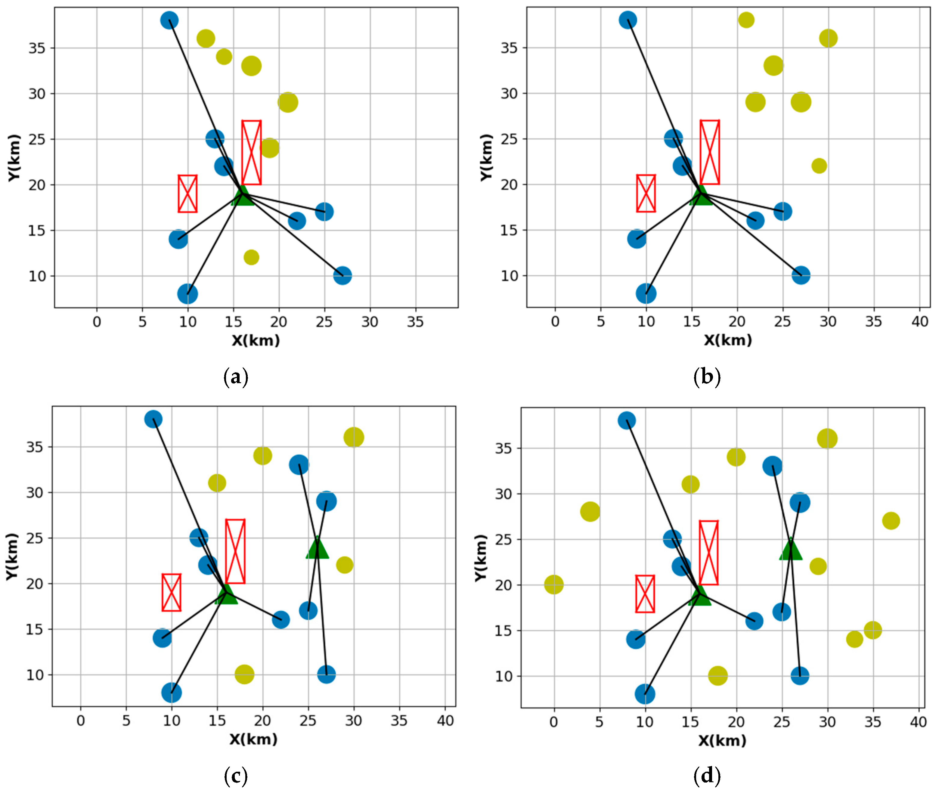
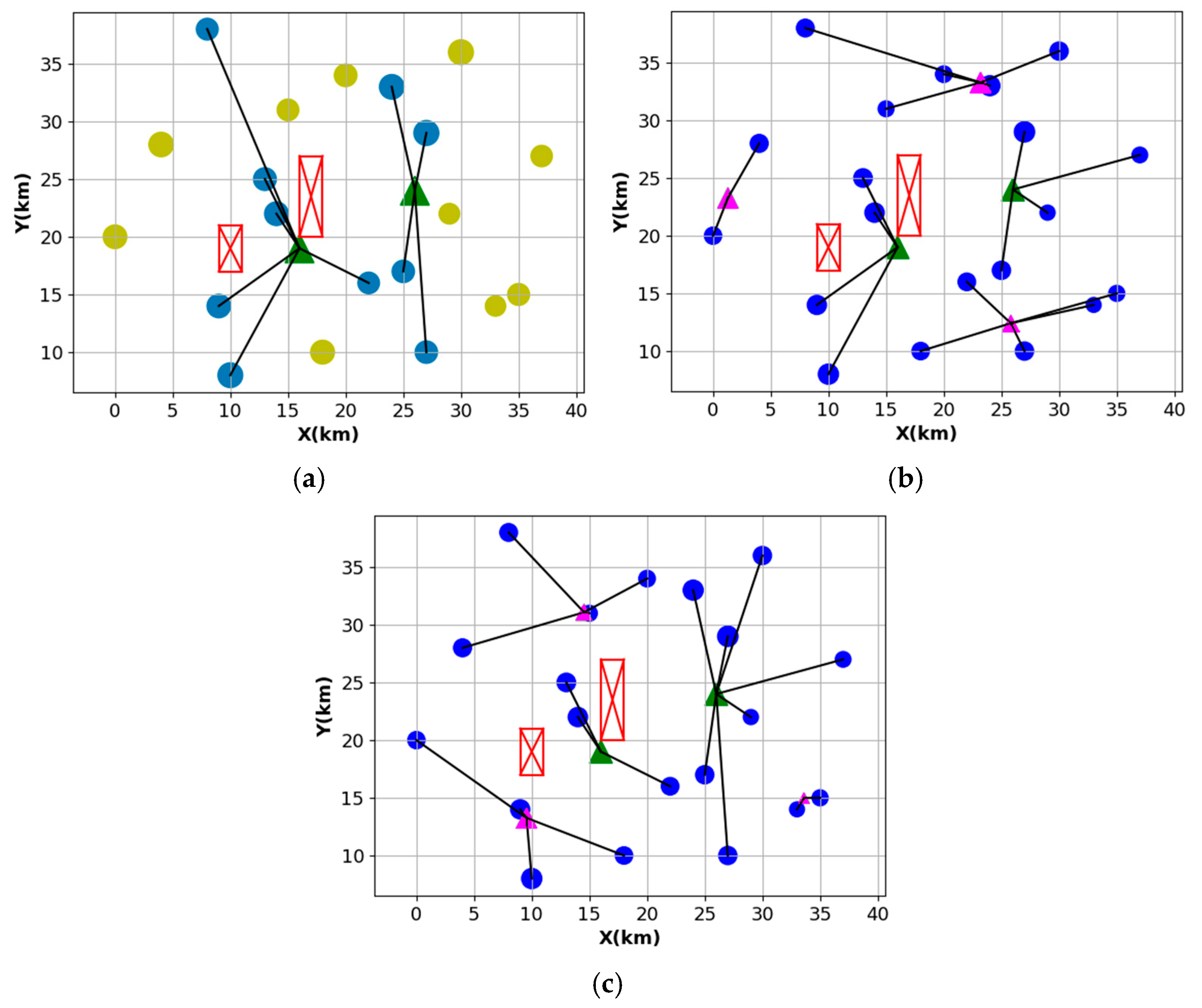
Figure 1.
Initial conditions of each scenario: (
a) Scenario A, (
b) Scenario B, (
c) Scenario C, and (
d) Scenario D. Source: Adapted from [
4].
Figure 1.
Initial conditions of each scenario: (
a) Scenario A, (
b) Scenario B, (
c) Scenario C, and (
d) Scenario D. Source: Adapted from [
4].
Figure 2.
Example of encoding vector with real values.
Figure 2.
Example of encoding vector with real values.
Figure 3.
Example of encoding vector with decimal values.
Figure 3.
Example of encoding vector with decimal values.
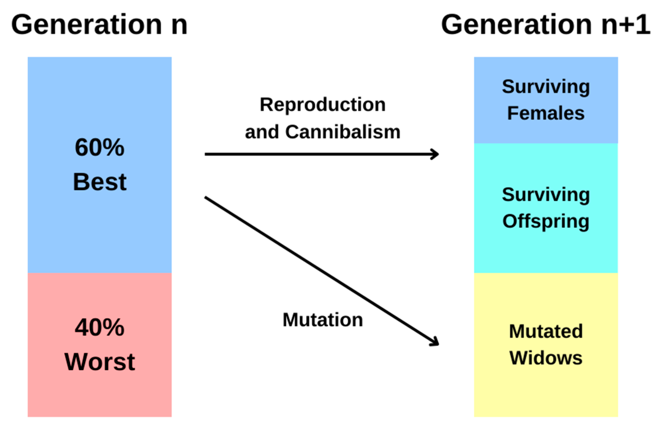
Figure 4.
Creation of a new generation of black widows.
Figure 4.
Creation of a new generation of black widows.
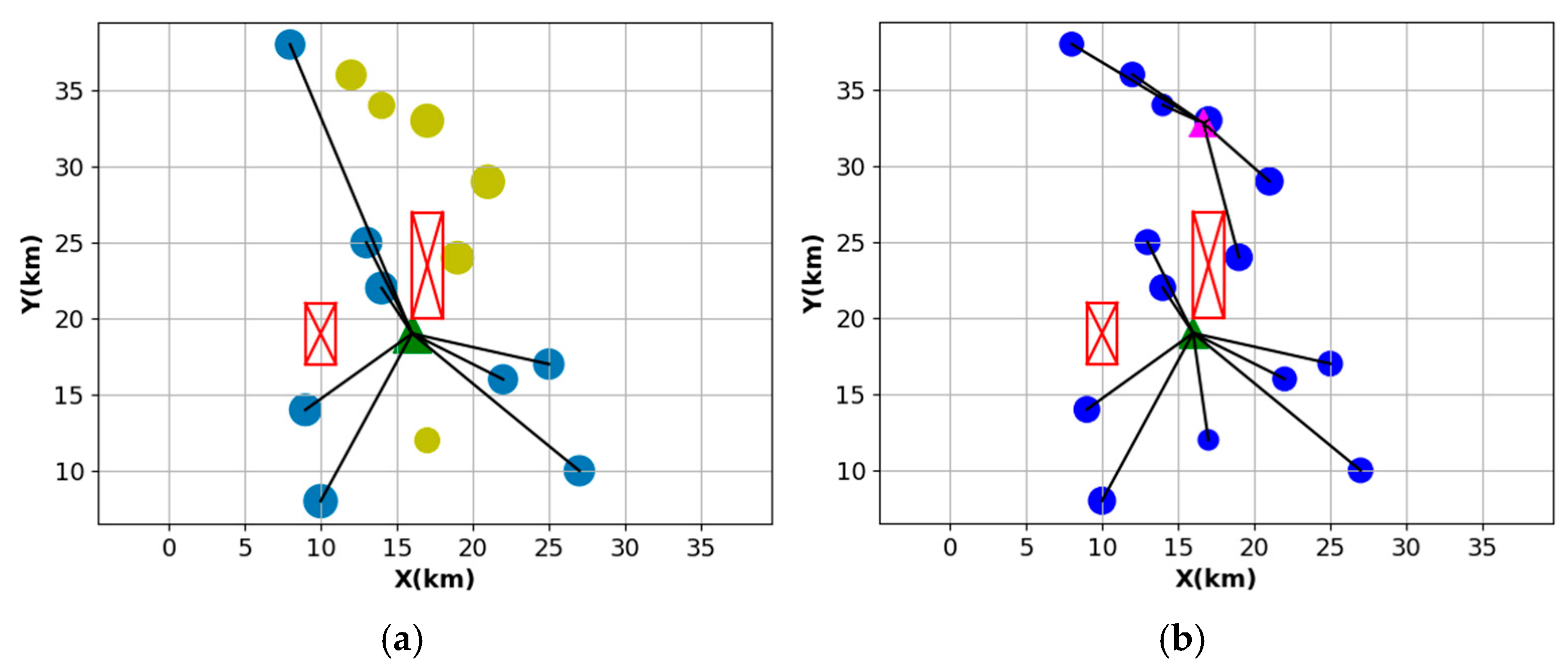
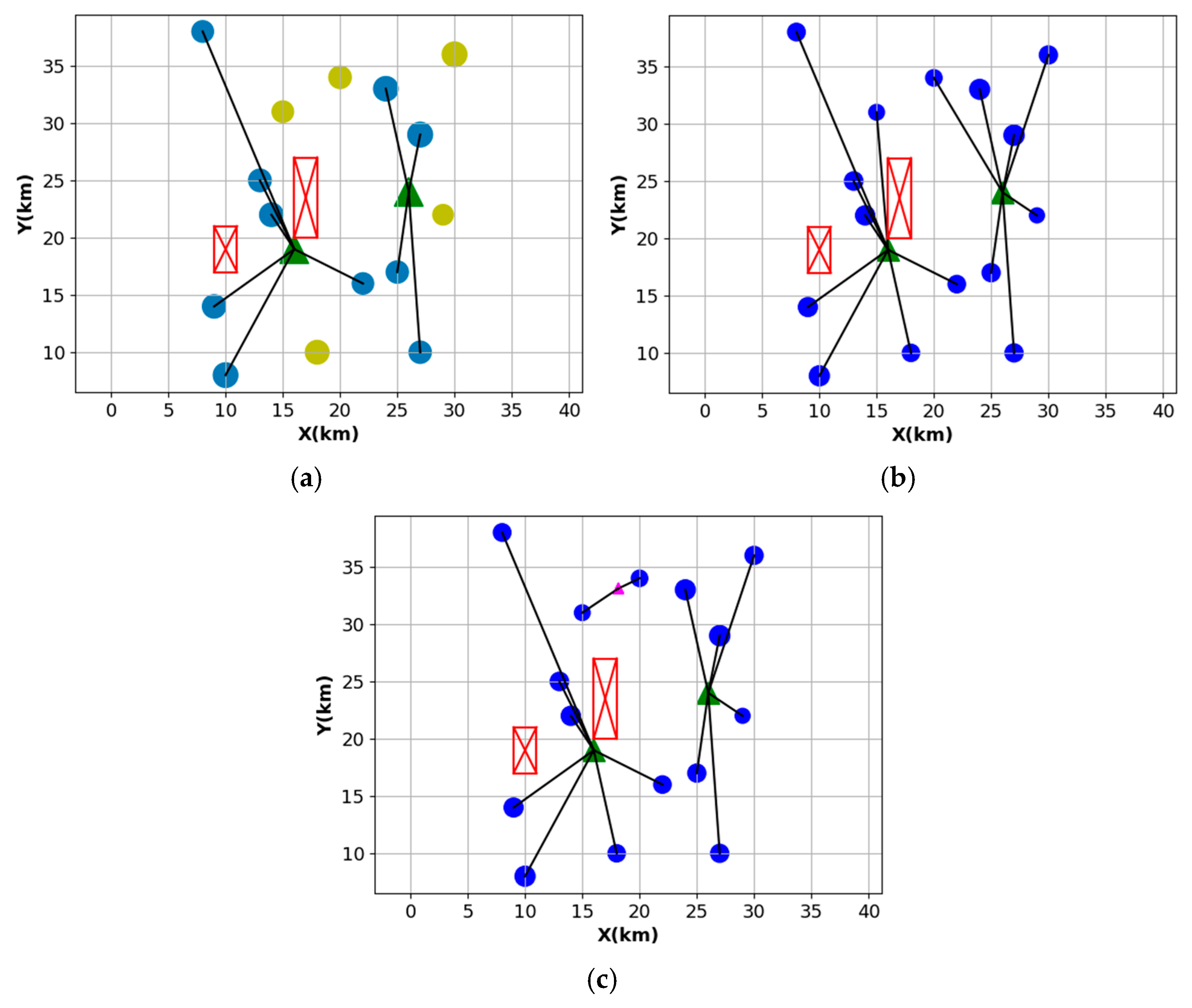
Figure 5.
Optimal solution found for Scenario A: (a) initial configuration and (b) optimal solution.
Figure 5.
Optimal solution found for Scenario A: (a) initial configuration and (b) optimal solution.
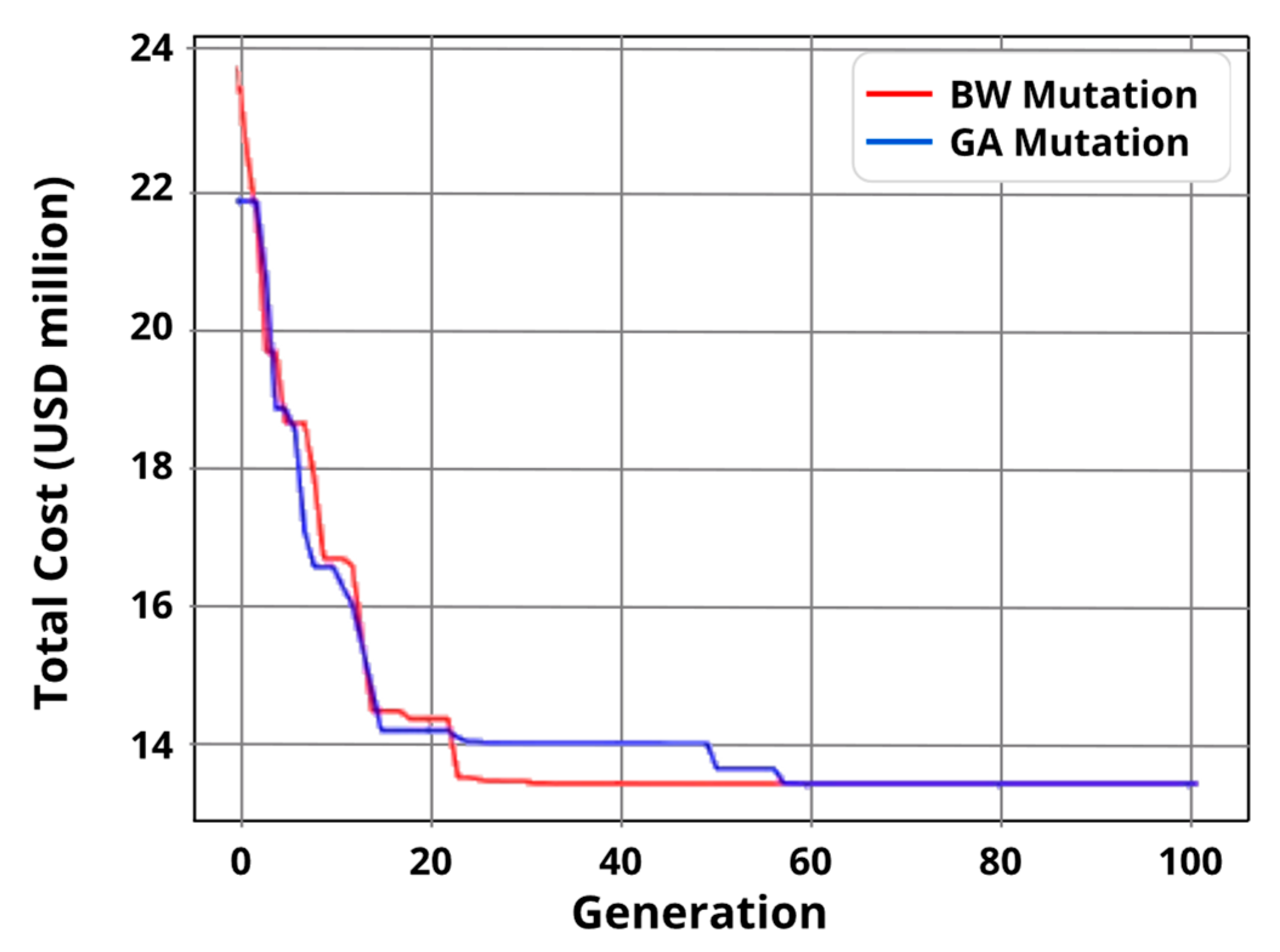
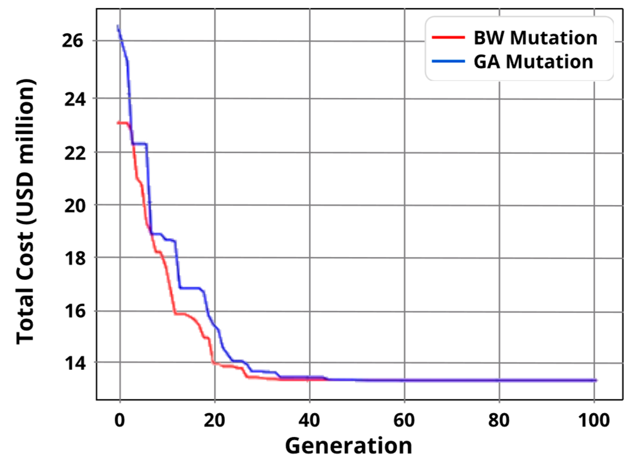
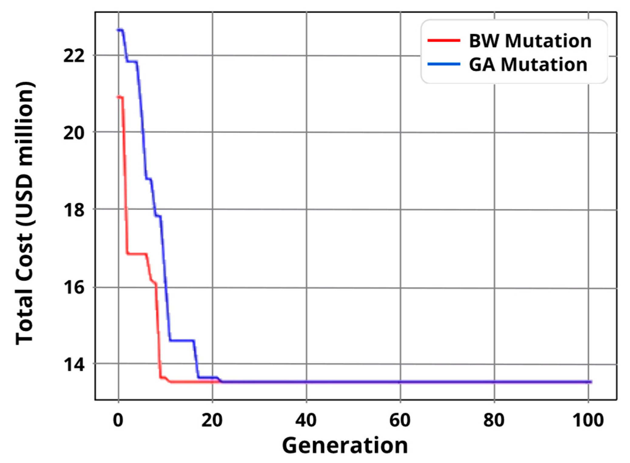
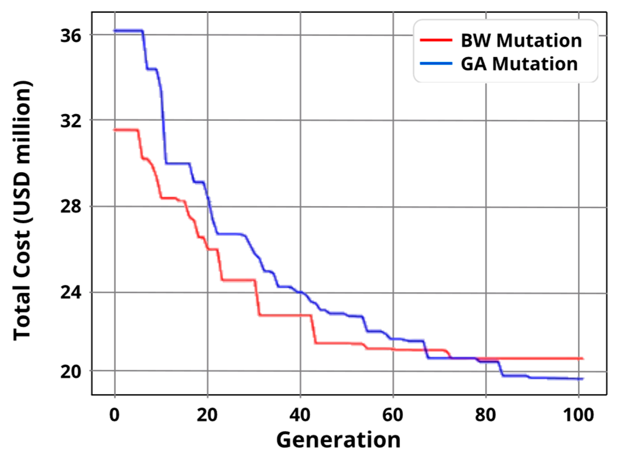
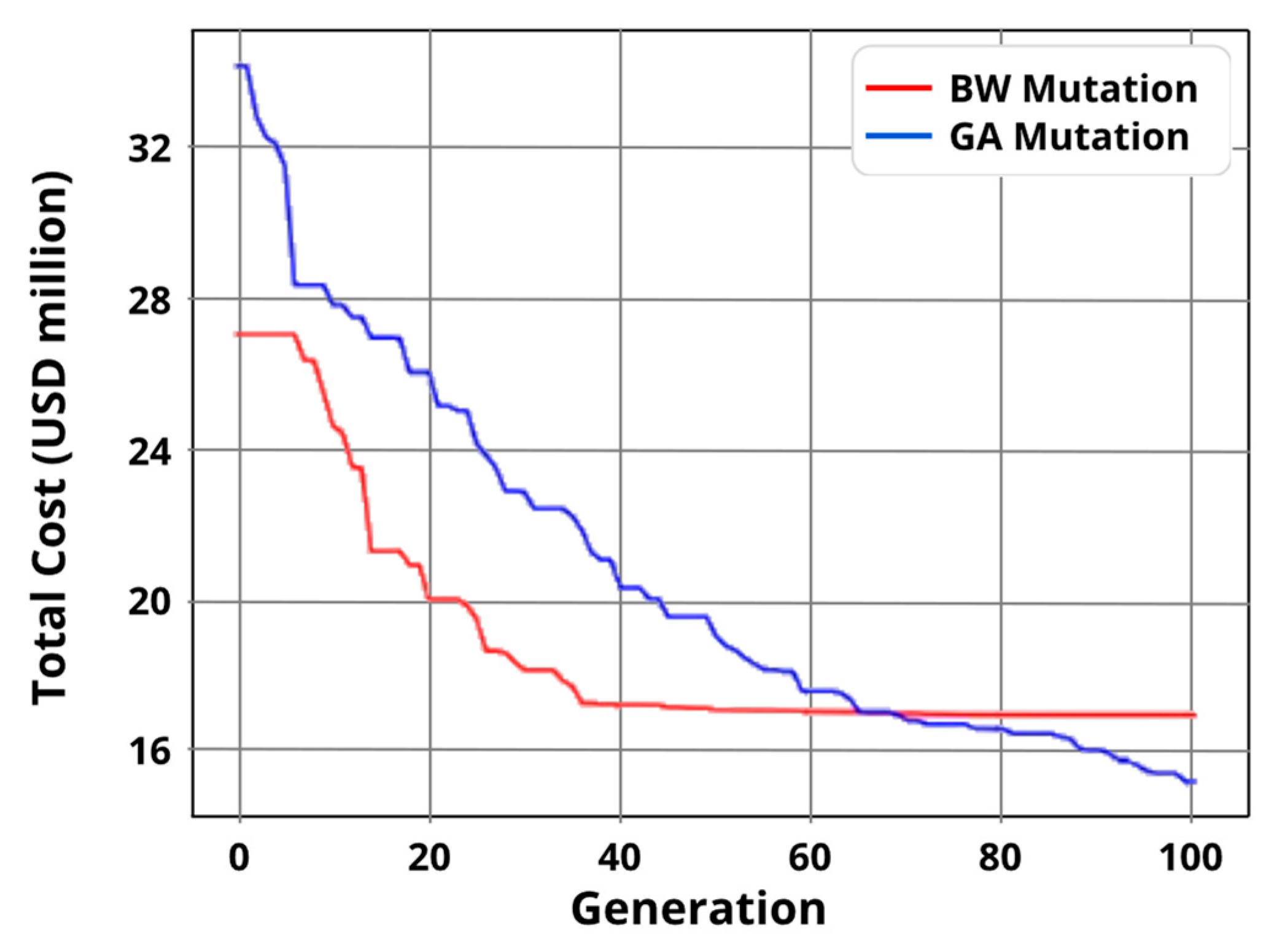
Figure 6.
Solution evolution for Scenario A.
Figure 6.
Solution evolution for Scenario A.
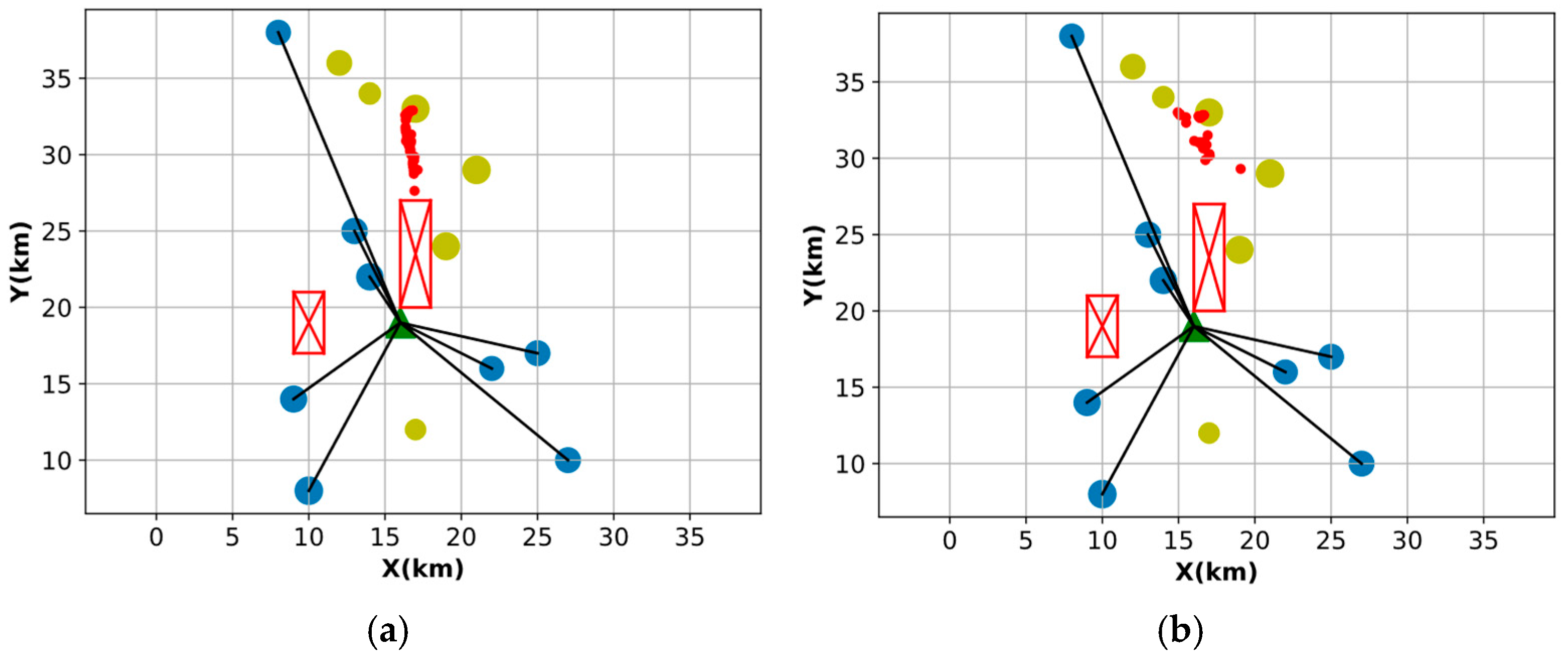
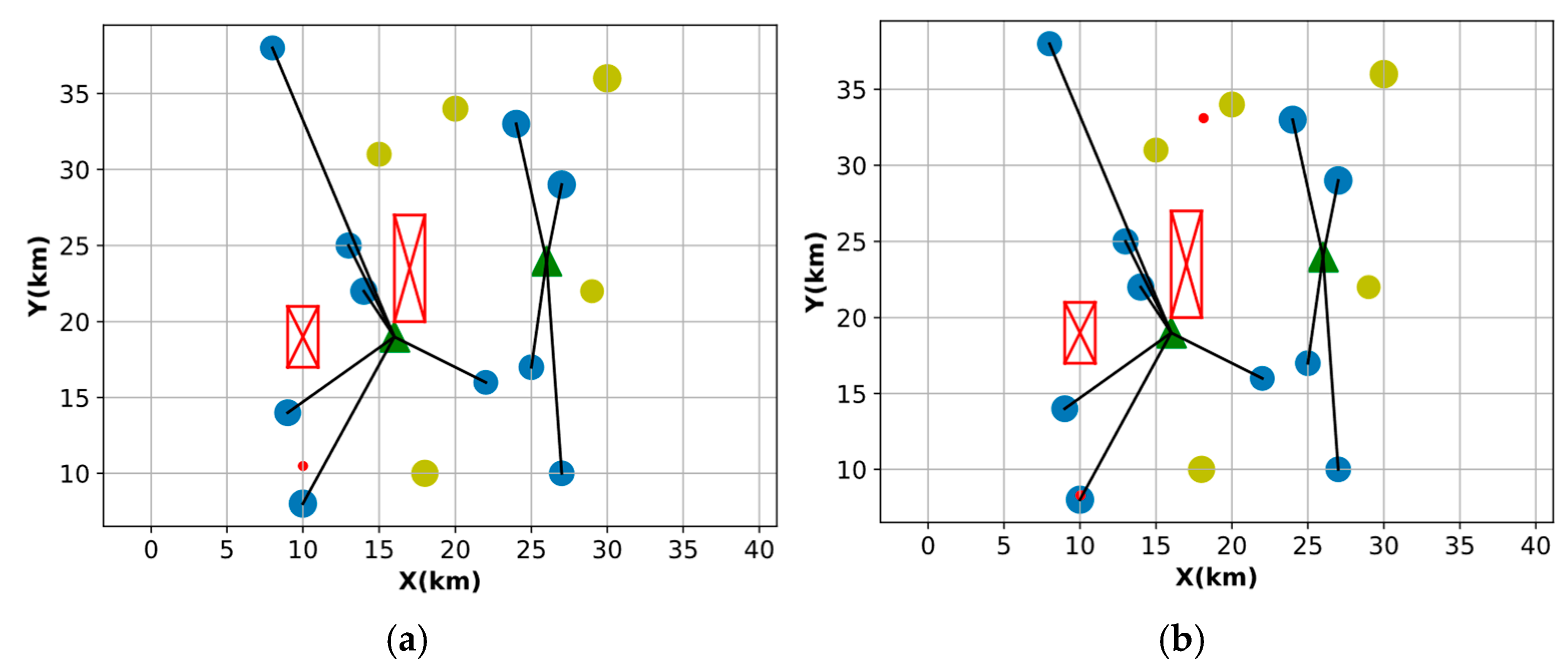
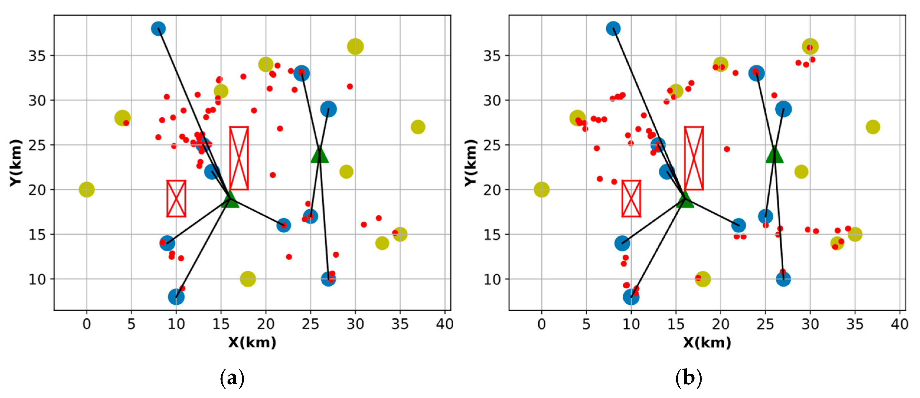
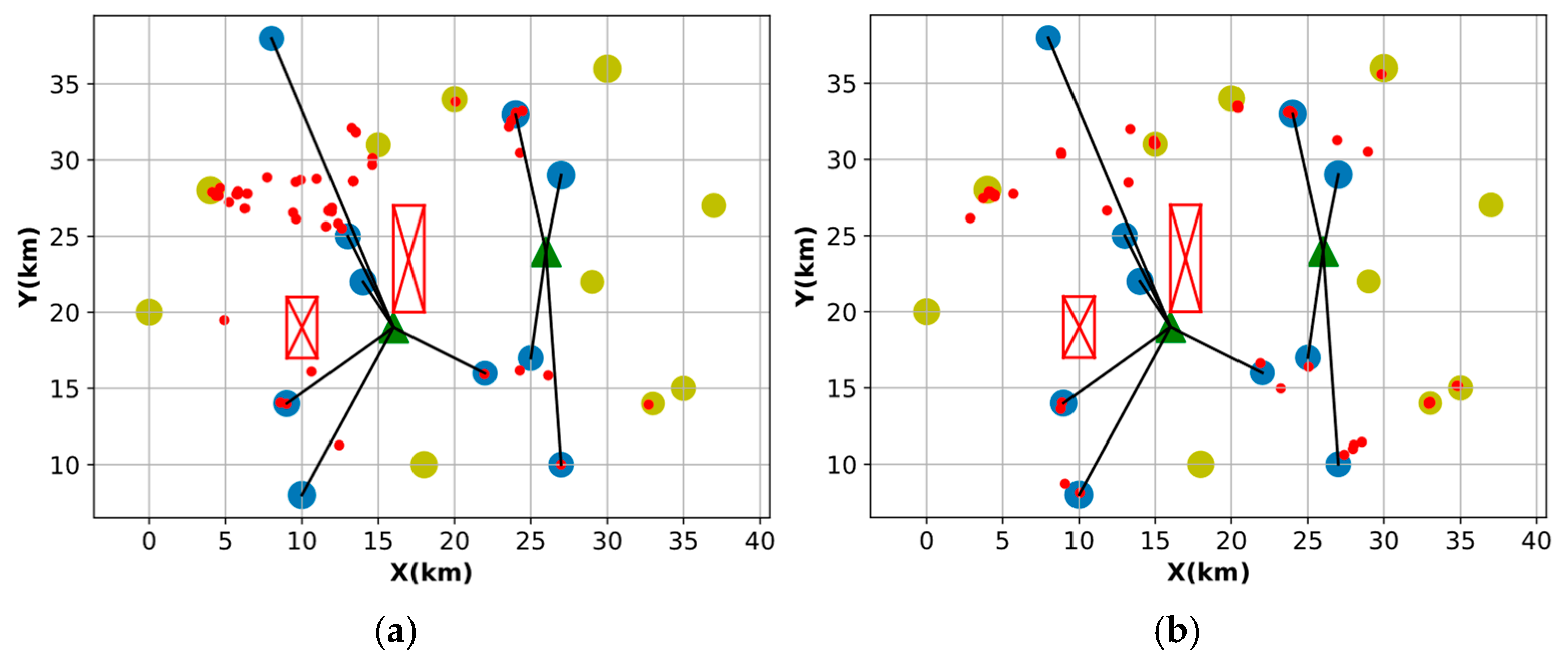
Figure 7.
Dispersion of new electrical substation positions for Scenario A: (a) BW mutation and (b) GA mutation.
Figure 7.
Dispersion of new electrical substation positions for Scenario A: (a) BW mutation and (b) GA mutation.
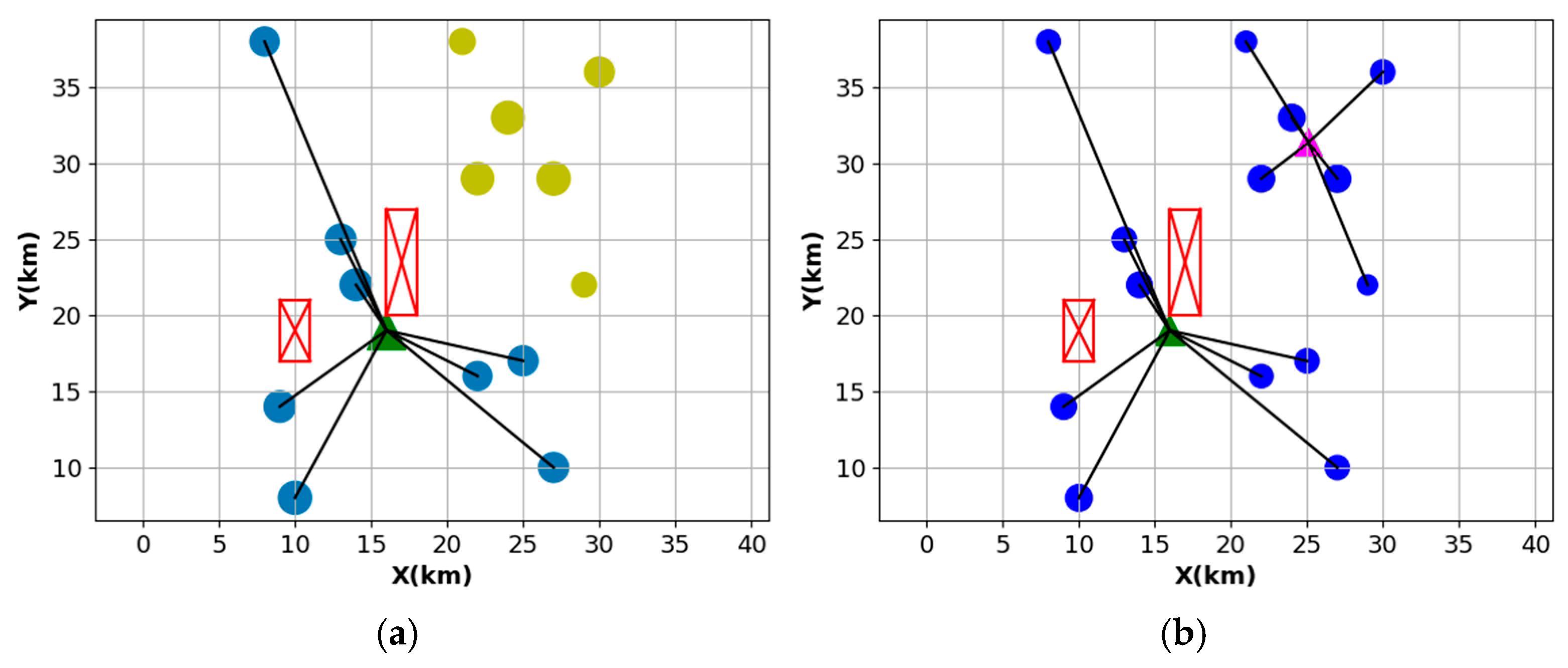
Figure 8.
Optimal solution found for Scenario B: (a) initial configuration and (b) optimal solution.
Figure 8.
Optimal solution found for Scenario B: (a) initial configuration and (b) optimal solution.
Figure 9.
Solution evolution for Scenario B.
Figure 9.
Solution evolution for Scenario B.
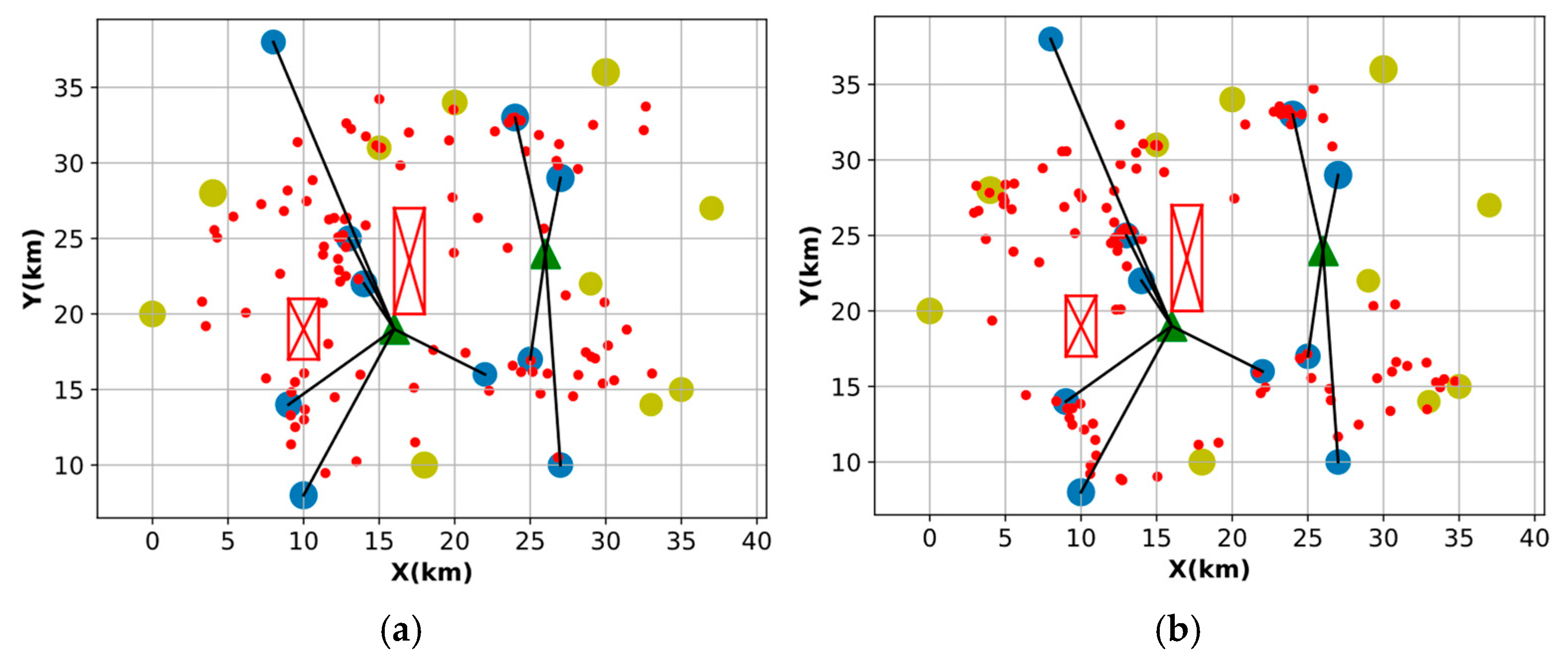
Figure 10.
Dispersion of new electrical substation positions for Scenario B: (a) BW mutation and (b) GA mutation.
Figure 10.
Dispersion of new electrical substation positions for Scenario B: (a) BW mutation and (b) GA mutation.
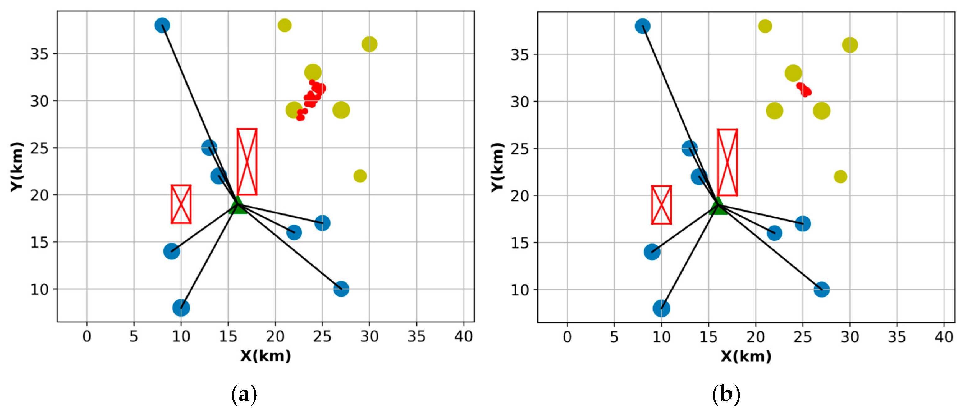
Figure 11.
Optimal solution found for Scenario C: (a) initial configuration, (b) optimal solution by BW mutation, and (c) optimal solution by GA mutation.
Figure 11.
Optimal solution found for Scenario C: (a) initial configuration, (b) optimal solution by BW mutation, and (c) optimal solution by GA mutation.
Figure 12.
Solution evolution for Scenario C.
Figure 12.
Solution evolution for Scenario C.
Figure 13.
Dispersion of new electrical substation positions for Scenario C: (a) BW mutation and (b) GA mutation.
Figure 13.
Dispersion of new electrical substation positions for Scenario C: (a) BW mutation and (b) GA mutation.
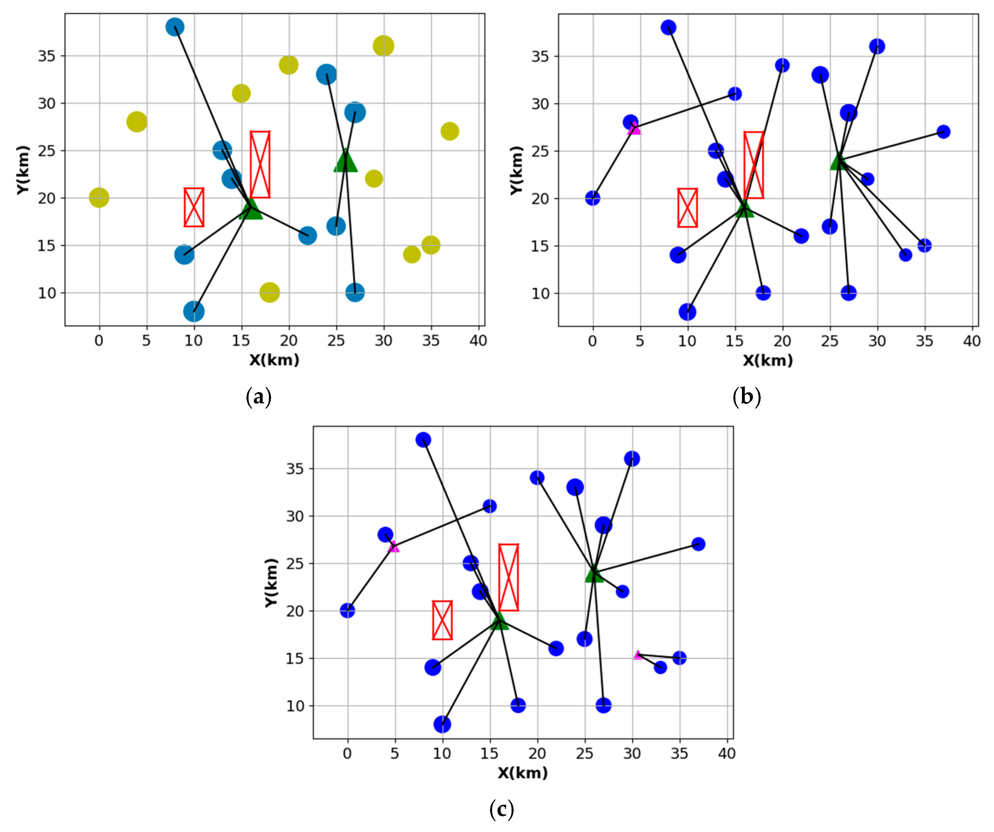
Figure 14.
Optimal solution found for Scenario D: (a) initial configuration, (b) optimal solution by BW mutation, and (c) optimal solution by GA mutation.
Figure 14.
Optimal solution found for Scenario D: (a) initial configuration, (b) optimal solution by BW mutation, and (c) optimal solution by GA mutation.
Figure 15.
Solution evolution for Scenario D.
Figure 15.
Solution evolution for Scenario D.
Figure 16.
Dispersion of new electrical substation positions for Scenario D: (a) BW mutation and (b) GA mutation.
Figure 16.
Dispersion of new electrical substation positions for Scenario D: (a) BW mutation and (b) GA mutation.
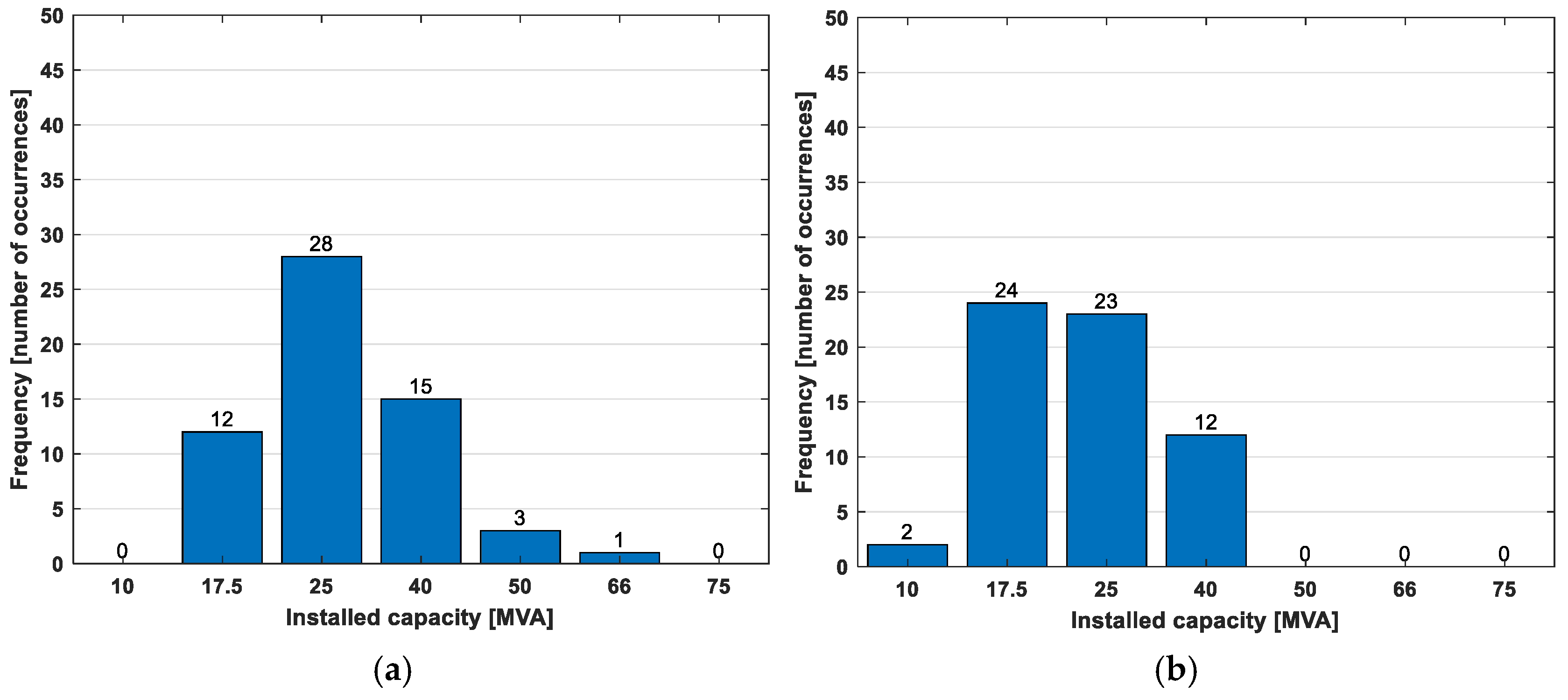
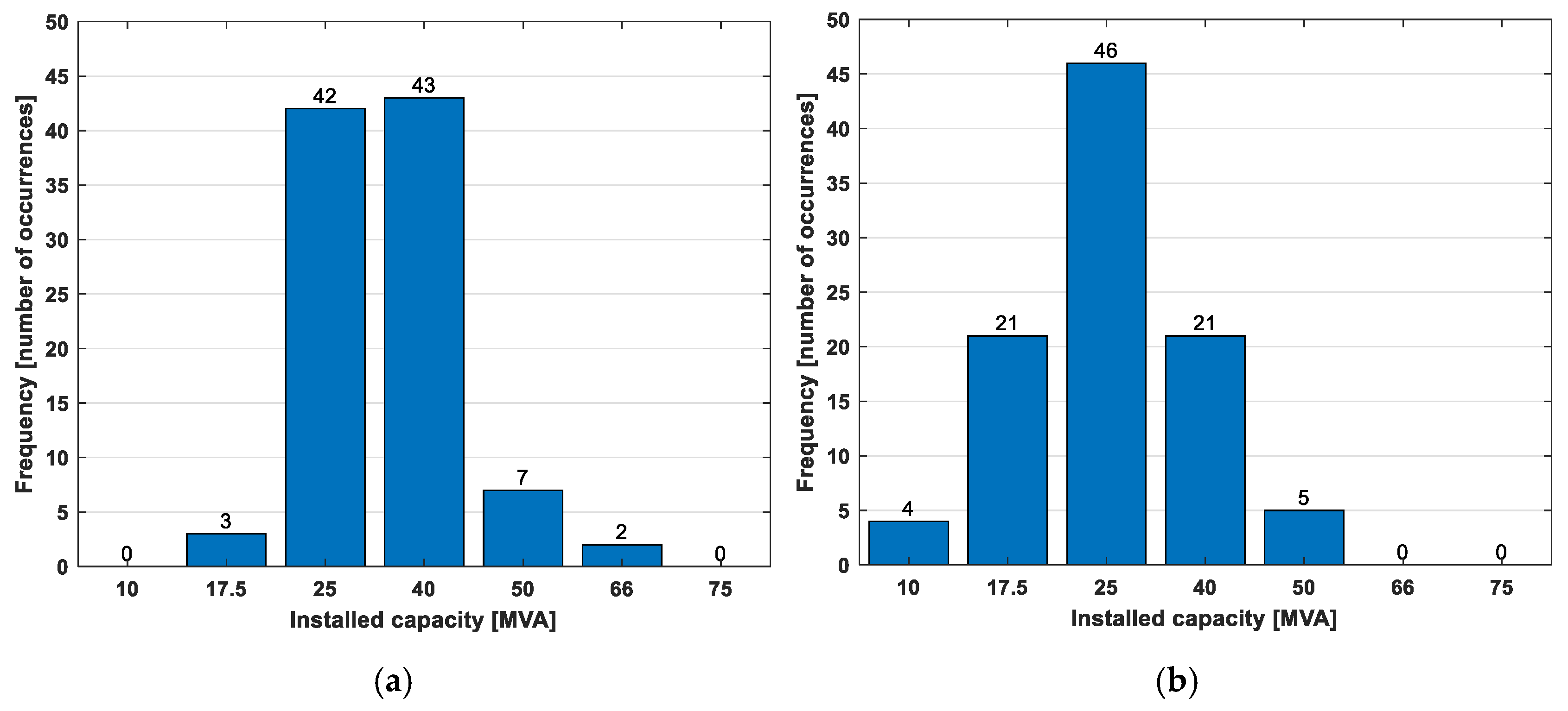
Figure 17.
Histograms of installed capacity for Scenario D (in some cases, more than one electrical substation was recommended by the algorithm in the same run): (a) BW mutation and (b) GA mutation.
Figure 17.
Histograms of installed capacity for Scenario D (in some cases, more than one electrical substation was recommended by the algorithm in the same run): (a) BW mutation and (b) GA mutation.
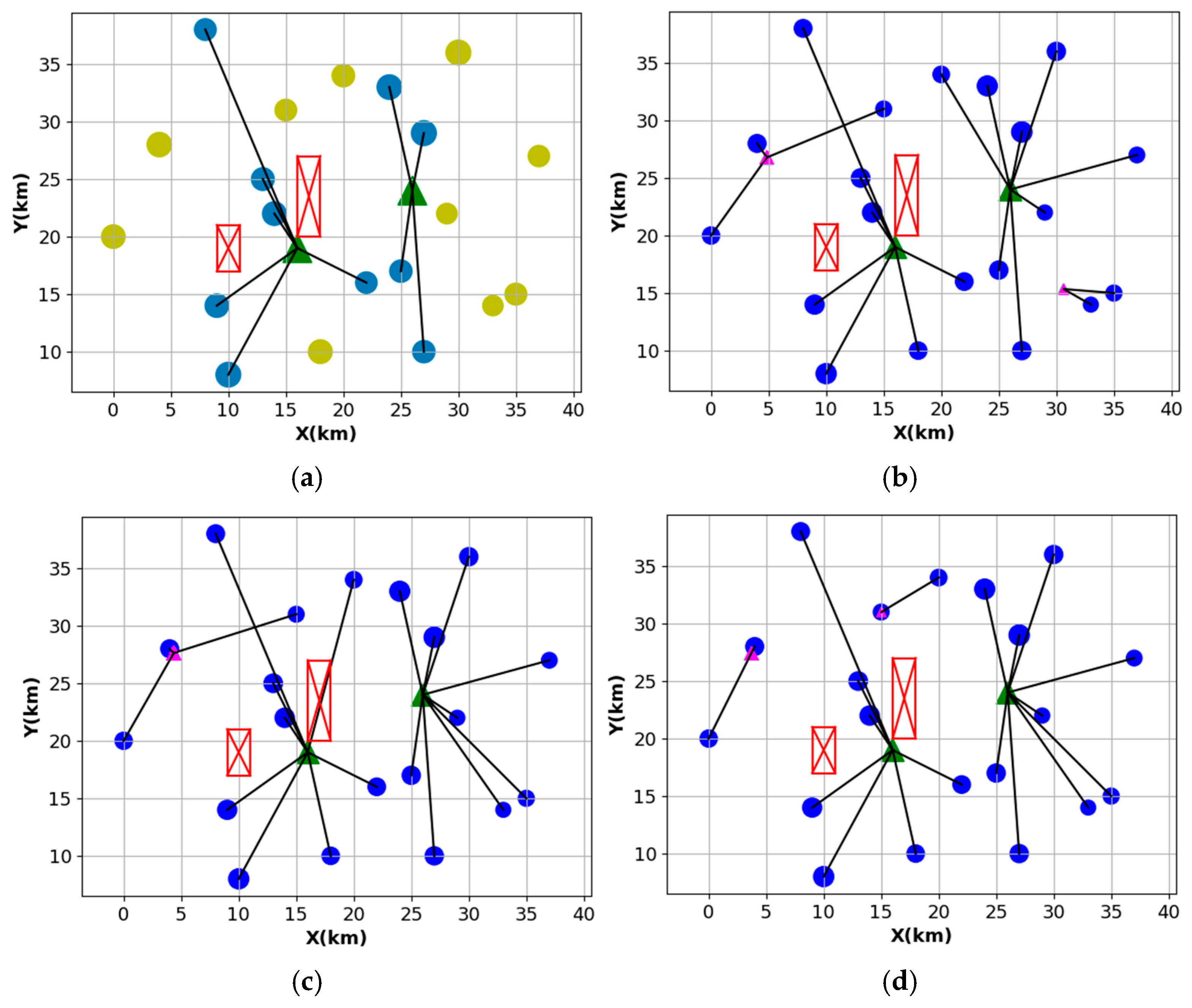
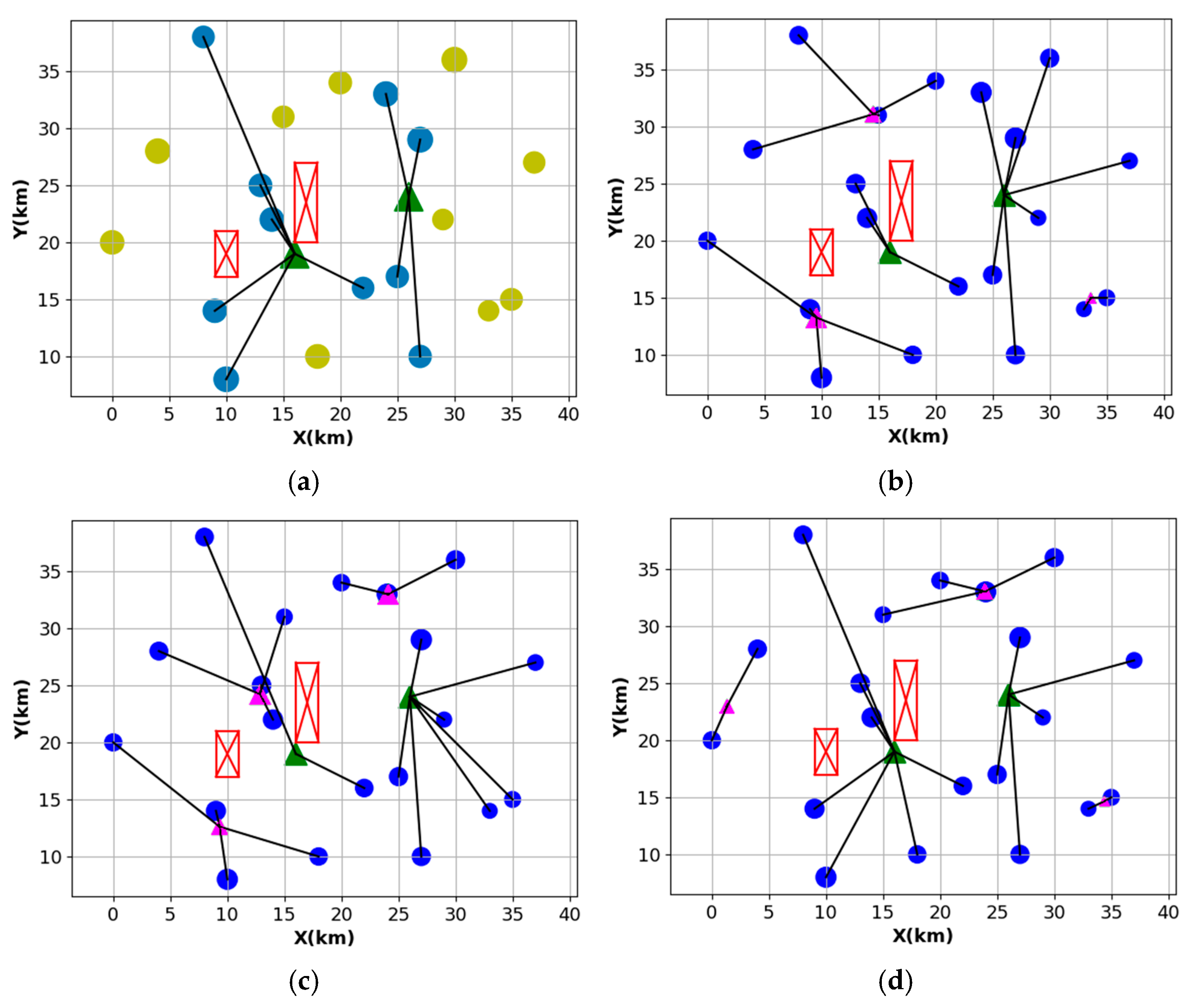
Figure 18.
Optimal solution found for Scenario D with 200 generations and black widows: (a) initial configuration, (b) optimal solution with 100 generations and black widows, (c) optimal solution by BW mutation with 200 generations and black widows, and (d) optimal solution by GA mutation with 200 generations and black widows.
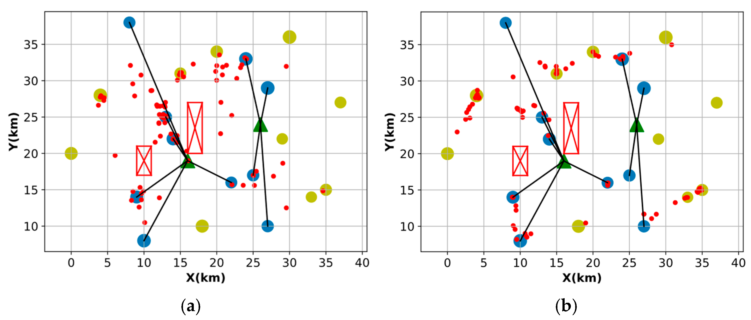
Figure 19.
Dispersion of new electrical substation positions for Scenario D with 200 generations and black widows: (a) BW mutation and (b) GA mutation.
Figure 19.
Dispersion of new electrical substation positions for Scenario D with 200 generations and black widows: (a) BW mutation and (b) GA mutation.
Figure 20.
Optimal solution found for Scenario D with reduced cost of electrical substations: (a) initial configuration, (b) optimal solution by BW mutation, and (c) optimal solution by GA mutation.
Figure 20.
Optimal solution found for Scenario D with reduced cost of electrical substations: (a) initial configuration, (b) optimal solution by BW mutation, and (c) optimal solution by GA mutation.
Figure 21.
Solution evolution for Scenario D with reduced electrical substation costs.
Figure 21.
Solution evolution for Scenario D with reduced electrical substation costs.
Figure 22.
Dispersion of new electrical substation positions for Scenario D with reduced electrical substation costs: (a) BW mutation and (b) GA mutation.
Figure 22.
Dispersion of new electrical substation positions for Scenario D with reduced electrical substation costs: (a) BW mutation and (b) GA mutation.
Figure 23.
Histograms of installed capacity for Scenario D (in some cases, more than one electrical substation was recommended by the algorithm in the same run) with reduced electrical substation costs: (a) BW mutation and (b) GA mutation.
Figure 23.
Histograms of installed capacity for Scenario D (in some cases, more than one electrical substation was recommended by the algorithm in the same run) with reduced electrical substation costs: (a) BW mutation and (b) GA mutation.
Figure 24.
Optimal solution found for Scenario D with reduced electrical substation costs and with 200 generations and black widows: (a) initial configuration, (b) optimal solution with 100 generations and black widows, (c) optimal solution by BW mutation with 200 generations and black widows, and (d) optimal solution by GA mutation with 200 generations and black widows.
Figure 25.
Dispersion of new electrical substation positions for Scenario D with reduced electrical substation costs and with 200 generations and black widows: (a) BW mutation and (b) GA mutation.
Figure 25.
Dispersion of new electrical substation positions for Scenario D with reduced electrical substation costs and with 200 generations and black widows: (a) BW mutation and (b) GA mutation.
Table 1.
Tested scenarios and their parameters.
Table 1.
Tested scenarios and their parameters.
| Scenario | Number of Generations and Black Widows | Electrical Substation Costs |
|---|
| A | 100 | 100% |
| B | 100 | 100% |
| C | 100 | 100% |
| D | 100 | 100% |
| D—200 | 200 | 100% |
| D mod. | 100 | 20% |
| D mod.—200 | 200 | 20% |
Table 2.
Costs of the optimal solution found in Scenario A.
Table 2.
Costs of the optimal solution found in Scenario A.
| Cost | Value (mi USD) |
|---|
| New electrical substations | 2.80 |
| New feeders | 2.54 |
| Power losses | 8.08 |
| Total value | 13.42 |
Table 3.
Cost values obtained after 50 runs for Scenario A.
Table 3.
Cost values obtained after 50 runs for Scenario A.
| Mutation | Optimal Value
(mi USD) | Average Value
(mi USD) | Standard Deviation
(mi USD) |
|---|
| BW | 13.42 | 13.75 | 0.23 |
| GA | 13.42 | 13.71 | 0.38 |
Table 4.
Costs of the optimal solution found in Scenario B.
Table 4.
Costs of the optimal solution found in Scenario B.
| Cost | Value (mi USD) |
|---|
| New electrical substations | 2.80 |
| New feeders | 2.08 |
| Power losses | 8.51 |
| Total value | 13.39 |
Table 5.
Cost values obtained after 50 runs for Scenario B.
Table 5.
Cost values obtained after 50 runs for Scenario B.
| Mutation | Optimal Value
(mi USD) | Average Value
(mi USD) | Standard Deviation
(mi USD) |
|---|
| BW | 13.39 | 13.47 | 0.16 |
| GA | 13.39 | 13.39 | 0.004 |
Table 6.
Costs of the optimal solution found in Scenario C.
Table 6.
Costs of the optimal solution found in Scenario C.
| Cost | Value (mi USD) |
|---|
| BW Mutation | GA Mutation | Δ (GA–BW) |
|---|
| New electrical substations | 0.00 | 1.60 | 1.60 |
| New feeders | 3.05 | 1.94 | −1.11 |
| Power losses | 10.24 | 9.74 | −0.50 |
| Total value | 13.29 | 13.28 | −0.01 |
Table 7.
Cost values obtained after 50 runs for Scenario C.
Table 7.
Cost values obtained after 50 runs for Scenario C.
| Mutation | Optimal Value
(mi USD) | Average Value
(mi USD) | Standard Deviation
(mi USD) |
|---|
| BW | 13.29 | 13.31 | 0.10 |
| GA | 13.28 | 13.30 | 0.06 |
Table 8.
Costs of the optimal solution found in Scenario D.
Table 8.
Costs of the optimal solution found in Scenario D.
| Cost | Value (mi USD) |
|---|
| BW Mutation | GA Mutation | Δ (GA–BW) |
|---|
| New electrical substations | 2.40 | 3.20 | 0.80 |
| New feeders | 6.07 | 5.01 | −1.06 |
| Power losses | 12.48 | 11.75 | −0.73 |
| Total value | 20.95 | 19.96 | −0.99 |
Table 9.
Cost values obtained after 50 runs for Scenario D.
Table 9.
Cost values obtained after 50 runs for Scenario D.
| Mutation | Optimal Value
(mi USD) | Average Value
(mi USD) | Standard Deviation
(mi USD) |
|---|
| BW | 20.95 | 22.29 | 1.49 |
| GA | 19.96 | 21.69 | 0.88 |
Table 10.
Costs of the optimal solution found in Scenario D with 200 generations and black widows.
Table 10.
Costs of the optimal solution found in Scenario D with 200 generations and black widows.
| Cost | Value (mi USD) |
|---|
| BW Mutation—200 Generations and Black Widows | GA Mutation—200 Generations and Black Widows | Δ (GA–BW) |
|---|
| New electrical substations | 2.00 | 3.60 | 1.60 |
| New feeders | 6.06 | 4.75 | −1.32 |
| Power losses | 12.48 | 11.44 | −1.04 |
| Total value | 20.55 | 19.79 | −0.75 |
Table 11.
Costs of the optimal solution found in Scenario D with 100 and 200 generations and black widows for the GA mutation.
Table 11.
Costs of the optimal solution found in Scenario D with 100 and 200 generations and black widows for the GA mutation.
| Cost | Value (mi USD) |
|---|
| GA Mutation—100 Generations and Black Widows | GA Mutation—200 Generations and Black Widows | Δ (GA 200—GA 100) |
|---|
| New electrical substations | 3.20 | 3.60 | 0.40 |
| New feeders | 5.01 | 4.75 | −0.26 |
| Power losses | 11.75 | 11.44 | −0.31 |
| Total value | 19.96 | 19.79 | −0.17 |
Table 12.
Cost values obtained after 50 runs for Scenario D with 100 and 200 generations and black widows for the BW and GA mutations.
Table 12.
Cost values obtained after 50 runs for Scenario D with 100 and 200 generations and black widows for the BW and GA mutations.
| Mutation | Optimal Value
(mi USD) | Average Value
(mi USD) | Standard Deviation
(mi USD) |
|---|
| BW—100 generations and black widows | 20.95 | 22.29 | 1.49 |
| BW—200 generations and black widows | 20.55 | 21.48 | 0.73 |
| GA—100 generations and black widows | 19.96 | 21.69 | 0.88 |
| GA—200 generations and black widows | 19.79 | 21.34 | 0.73 |
Table 13.
Costs of the optimal solution found in Scenario D with reduced electrical substation costs.
Table 13.
Costs of the optimal solution found in Scenario D with reduced electrical substation costs.
| Cost | Value (mi USD) |
|---|
| BW Mutation | GA Mutation | Δ (GA–BW) |
|---|
| New electrical substations | 2.08 | 1.36 | −0.72 |
| New feeders | 5.18 | 4.64 | −0.54 |
| Power losses | 9.50 | 9.35 | −0.15 |
| Total value | 16.76 | 15.35 | −1.41 |
Table 14.
Cost values obtained after 50 runs for Scenario D with reduced electrical substation costs.
Table 14.
Cost values obtained after 50 runs for Scenario D with reduced electrical substation costs.
| Mutation | Optimal Value
(mi USD) | Average Value
(mi USD) | Standard Deviation
(mi USD) |
|---|
| BW | 16.76 | 19.93 | 1.18 |
| GA | 15.35 | 18.30 | 1.21 |
Table 15.
Costs of the optimal solution found in Scenario D with reduced electrical substation costs and with 200 generations and black widows.
Table 15.
Costs of the optimal solution found in Scenario D with reduced electrical substation costs and with 200 generations and black widows.
| Cost | Value (mi USD) |
|---|
| BW Mutation—200 Generations and Black Widows | GA Mutation—200 Generations and Black Widows | Δ (GA–BW) |
|---|
| New electrical substations | 1.60 | 1.20 | −0.40 |
| New feeders | 6.06 | 3.44 | −2.62 |
| Power losses | 9.00 | 9.57 | 0.57 |
| Total value | 16.66 | 14.21 | −2.46 |
Table 16.
Costs of the optimal solution found in Scenario D with reduced electrical substation costs and with 100 and 200 generations and black widows for the GA mutation.
Table 16.
Costs of the optimal solution found in Scenario D with reduced electrical substation costs and with 100 and 200 generations and black widows for the GA mutation.
| Cost | Value (mi USD) |
|---|
| GA Mutation—100 Generations and Black Widows | GA Mutation—200 Generations and Black Widows | Δ (GA 200—GA 100) |
|---|
| New electrical substations | 1.36 | 1.20 | −0.16 |
| New feeders | 4.64 | 3.44 | −1.20 |
| Power losses | 9.35 | 9.57 | 0.23 |
| Total value | 15.35 | 14.21 | −1.14 |
Table 17.
Cost values obtained after 50 runs for Scenario D with reduced electrical substation costs and with 100 and 200 generations and black widows for the BW and GA mutation.
Table 17.
Cost values obtained after 50 runs for Scenario D with reduced electrical substation costs and with 100 and 200 generations and black widows for the BW and GA mutation.
| Mutation | Optimal Value
(mi USD) | Average Value
(mi USD) | Standard Deviation
(mi USD) |
|---|
| BW—100 generations and black widows | 16.76 | 19.93 | 1.18 |
| BW—200 generations and black widows | 16.66 | 19.37 | 0.88 |
| GA—100 generations and black widows | 15.35 | 18.30 | 1.21 |
| GA—200 generations and black widows | 14.21 | 17.63 | 1.65 |
Table 18.
Comparison of the optimal solutions found in each scenario.
Table 18.
Comparison of the optimal solutions found in each scenario.
| Scenario | Value (mi USD) |
|---|
| BW Mutation | GA Mutation | Δ (GA–BW) |
|---|
| A | 13.42 | 13.42 | - |
| B | 13.39 | 13.39 | - |
| C | 13.29 | 13.28 | −0.08 % |
| D | 20.95 | 19.96 | −4.73 % |
| D—200 | 20.55 | 19.79 | −3.67% |
| D mod. | 16.76 | 15.35 | −8.41% |
| D mod.—200 | 16.66 | 14.21 | −14.75% |
Table 19.
Comparison of the average solutions found in each scenario.
Table 19.
Comparison of the average solutions found in each scenario.
| Scenario | Value (mi USD) |
|---|
| BW Mutation | GA Mutation | Δ (GA–BW) |
|---|
| A | 13.75 | 13.71 | −0.23% |
| B | 13.47 | 13.39 | −0.58% |
| C | 13.31 | 13.30 | −0.09% |
| D | 22.29 | 21.69 | −2.68% |
| D—200 | 21.48 | 21.34 | −0.66% |
| D mod. | 19.93 | 18.30 | −8.17% |
| D mod.—200 | 19.37 | 17.63 | −9.00% |


