Microgrid Multivariate Load Forecasting Based on Weighted Visibility Graph: A Regional Airport Case Study

Abstract

This paper introduces an alternative forecasting approach that leverages the application of visibility graphs in the context of multivariate energy forecasting for a regional airport, which incorporates energy demand of diverse types of buildings and wind power generation. The motivation for this research stems from the urgent need to enhance the accuracy and reliability of load forecasting in microgrids, which is crucial for optimizing energy management, integrating renewable sources, and reducing operational costs, thereby contributing to more sustainable and efficient energy systems. The proposed methodology employs visibility graph transformations, the superposed random walk method, and temporal decay adjustments, where more recent observations are weighted more significantly to predict the next time step in the data set. The results indicate that the proposed method exhibits satisfactory performance relative to comparison models such as Exponential smoothing, ARIMA, Light Gradient Boosting Machine and CNN-LSTM. The proposed method shows improved performance in forecasting energy consumption for both stationary and highly variable time series, with SMAPE and NMRSE values typically in the range of 4–10% and 5–20%, respectively, and an $R^2$ reaching 0.96. The proposed method affords notable benefits to the forecasting of energy demand, offering a versatile tool for various kinds of structures and types of energy production in a microgrid. This study lays the groundwork for further research and real-world applications within this field by enhancing both the theoretical and practical aspects of time series forecasting, including load forecasting.

1. Introduction

Microgrids play a pivotal role in sustainable energy solutions by offering localized energy management and integration of renewable energy systems [1]. These systems are indispensable in specialized environments, such as campuses, industrial sites, and airports, where the diverse energy demands and operational constraints necessitate effective management [2]. The precision in load forecasting for microgrids can result in resource optimization, cost reduction, and reliable energy supply, thus minimizing outages [3]. Nonetheless, the task of energy forecasting in microgrids is highly intricate due to the multivariate dynamics that encompass numerous factors [4].

Airports encompass various types of structures, including passenger terminals, maintenance centers, and administrative offices, each exhibiting distinct energy usage patterns subject to influences such as operational schedules, climatic conditions, occupancy levels, and the deployment of equipment [5,6]. The energy demands of terminals are particularly impacted by flight timetables and passenger volume fluctuations, while maintenance facilities consistently demonstrate substantial energy consumption [7]. The variability inherent in load profiles complicates the reliability of energy forecasts, highlighting their critical importance [8].

Traditional forecasting models such as autoregressive (AR) models, autoregressive integrated moving average (ARIMA), and their variants have been commonly applied to predict energy consumption and generation patterns [9]. Despite their ability to capture linear dependencies and stationary processes, these models fail when real-world data present complexity, non-linearity, and non-stationarity [10].

On the other hand, machine learning techniques, such as support vector machines (SVMs), random forests, and neural networks, have introduced a data-driven paradigm in energy forecasting [11]. These models can handle higher-dimensional data and incorporate non-linear relationships, offering improved accuracy over purely statistical methods. However, the multivariate nature of microgrid data, which is characterized by multiple interrelated variables such as weather conditions, building-specific energy consumption patterns, and operational schedules, poses additional challenges. Recent airport prediction studies employed several machine learning techniques, including Multi-layer Perceptron (MLP), Long Short-Term Memory (LSTM), and Bidirectional-LSTM by Vontzos et al. [12], singular spectrum analysis with a CNN-Transformer by Chen et al. [13], and a particle swarm optimized gated recurrent unit (GRU) by Song et al. [14]. Conventional machine learning models often require extensive feature engineering and are limited in their ability to fully capture multiscale and long-range dependencies between variables [15,16].

To address these challenges, recent advances in energy forecasting have increasingly focused on hybrid approaches and advanced data-driven techniques [17]. These methods combine the strengths of traditional models with modern innovations in computational intelligence and data representation. Among these innovations, the integration of graph theory into time series analysis has emerged as a promising direction [18].

Lacasa et al. [19] introduced a novel graph-theoretic method that transforms time series data into networks using visibility graphs (VGs). VGs identify temporal patterns, non-linear dependencies, and long-range correlations within time series data [20]. VG-based methodologies make use of the graph structure to analyze the interconnectedness of data points and reveal patterns that may not be apparent in the raw time series, in contrast to traditional methods that treat time series data as a sequence of independent observations. The visibility graph technique was initially designed for univariate data. VGs are also suitable for multivariate cases [21,22], by constructing individual visibility graphs for each variable or by developing joint visibility graphs that account for interactions between variables. Using VGs, researchers can effectively model the dependencies across diverse data streams. This capability is particularly useful for predicting energy consumption in airport microgrid systems, where energy forecasting involves integrating information from heterogeneous sources such as weather forecasts, renewable energy generation profiles, and building-specific energy demand.

Visibility graphs find applications in numerous research fields, including human health [23,24], financial analysis [25,26], environmental studies [27,28], physics [29], transportation [30,31], and image processing [32,33]. Recent studies have used visibility graphs for energy forecasting [34], showing that they outperform typical machine learning methods in this domain.

Zhang et al. [35] contributed a major advancement by applying complex networks to time series forecasting first. Their algorithm mapped time series into a visibility graph, calculated node similarities using local random walks, and generated predictions by weighting initial forecasts with fuzzy rules. Various researchers were inspired by this pioneering work, such as Mao and Xiao [36], who improved the predictions by refining the similarity measure and introducing distance-based weighting. Liu and Deng [37] incorporated weighted sums of slopes between multiple similar nodes for greater accuracy. Zhao et al. [38] proposed an efficient method that utilizes the slopes of all nodes visible from the last node, taking into account the degree of the node and the temporal distance to obtain the final weighted result. Zhan and Xiao [39] enhanced prior researchers’ work by transforming node similarity into a weight for weighted predictions on forecasted values from various nodes. These works highlight the flexibility of VG-based forecasting methods and their progress in capturing the geometric and temporal characteristics of time series.

This study introduces a different forecasting methodology that utilizes the visibility graph approach within the context of multivariate energy forecasting for a microgrid. This novel technique aims to improve forecast accuracy by incorporating complex network theory, which offers a promising alternative to conventional forecasting methods in energy management systems, using the superposed random walk approach proposed by Zhan and Xiao [39] by integrating temporal weighting. It highlights the advantages, challenges, and future prospects of using these advanced methods for real-world energy forecasting problems. The proposed algorithm contributes as follows:

• Using the superposed random walk approach, the algorithm generates a similarity matrix that captures both local and global structural relationships inherent in the visibility graph, which is constructed from the multivariate time series data.
• A temporal decay factor is introduced to regulate the effect of historical data points, ensuring that more recent observations in the time series are weighted more significantly in the forecasting process.
• The algorithm integrates similarity scores with decay factors, forming a normalized weight vector. This vector balances structural and temporal information, improving the ability of the forecasting model to handle various patterns in the microgrid’s energy and environmental data.
• Forecasts for each time step are generated using weighted aggregation of node predictions, where weights are derived from the adjusted similarity scores. This ensures that the algorithm prioritizes the most relevant data points while minimizing the impact of noise or irrelevant historical patterns.
• The methodology is validated on the multivariate time series of an airport microgrid, which includes variables such as the energy demand of versatile buildings and wind power generation with time series that present different time dependency and seasonality.

The proposed algorithm utilizing visibility graphs offers a unique advantage in transforming time series data into a network structure, which allows for the uncovering of hidden patterns and relationships that traditional machine learning models might overlook. Additionally, the algorithm demonstrates superior performance in predicting energy usage in time series presenting stationarity and high variability. These contributions highlight the adaptability and robustness of the algorithm, making it a promising tool for forecasting in complex, multivariate environments such as airport microgrids, where energy consumption patterns are influenced by multiple interdependent factors.

This paper has been divided into the following parts. Section 2 introduces and analyzes the necessary actions related to graph computation techniques and presents the forecasting model. The description of the data set, preprocessing, the experiments conducted, and their results are presented in Section 3. In Section 4, the results and limitations are discussed, while some directions for future work are suggested. In Section 5, we conclude with the main findings of our work.

2. Materials and Methods

2.1. Preliminaries

The estimation of power usage in microgrid buildings alongside the generation of energy from renewable sources can be analyzed as a problem involving predictions across multiple variables. To formulate multivariate forecasting using a visibility graph (VG), we represent the time series data from multiple variables as a graph structure and utilize it for prediction.

Consider a multivariate time series, $X\left(t\right)$, with n variables:

$$X\left(t\right)=\left[\begin{array}{c}{x}_1\left(t\right)\\ x_2\left(t\right)\\ ⋮\\ x_n\left(t\right)\end{array}\right],t=1,2,\dots ,T,$$

(1)

where $x_i\left(t\right)$ represents the value of the i-th variable at time t, and T is the total number of time steps. Each time series is symbolized as

$$x_i\left(t\right)=\{(t_1,x_i\left(t_1\right)),(t_2,x_i\left(t_2\right)),\dots ,(t_T,x_i\left(t_T\right))\}$$

(2)

while i-th variable prediction is formulated as

$${\widehat{x}}_i(T+1)=w_i\ast F_i$$

(3)

where $w_i$ and $F_i$ are the weight and forecasting vectors, respectively.

2.2. Visibility Graph

The visibility graph (VG) method transforms a time series into a network by assigning each data point as a node and establishing connections (edges) between nodes based on a visibility criterion, where a direct line connecting two points does not intersect any intermediate data points.

For each time series, $x_i\left(t\right)$ (Equation (2)), a visibility graph, $G_i=(V_i,E_i)$, is constructed, where $V_i=\{v_1,v_2,\dots ,v_T\}$ represents the nodes corresponding to the time points t, while $E_i$ represents the edges defined by the visibility criterion between the time points $t_a$ and $t_b$ ($t_a<t_b$), where $x_i\left(t_a\right),x_i\left(t_b\right)$ are visible if Equation (4) is satisfied [19], which ensures that no intermediate points block visibility between nodes:

$$x_i\left(t_c\right)<x_i\left(t_a\right)+{\displaystyle \frac{t_c-t_a}{t_b-t_a}}\left(x_i\left(t_b\right)-x_i\left(t_a\right)\right),\forall t_c\in (t_a,t_b).$$

(4)

Additionally, VG provides an adjacency matrix, A, where each element, $A_{ij}$, is 1 if there is an edge between nodes i and j; otherwise it is 0.

$$A=\left[\begin{array}{cccc}{a}_{11}& a_{12}& \dots & a_{1n}\\ a_{21}& a_{22}& \dots & a_{2n}\\ ⋮& ⋮& \ddots & ⋮\\ a_{n1}& a_{n2}& \dots & a_{nn}\end{array}\right]$$

(5)

2.3. Superposed Random Walk

The superposed random walk (SRW) method is a technique used to compute similarity between nodes in a graph [40]. This similarity is particularly useful for tasks like link prediction and, in this context, forecasting in time series data converted into a visibility graph. The SRW method leverages the random walk process on a graph to iteratively calculate the similarity between nodes. It considers not only the direct connections between nodes, but also the cumulative influence of longer paths. By superposing multiple random walk steps, the method captures both local and global structural relationships within the graph.

Initially, a time series is transformed into an undirected visibility graph, as described in Section 2.2. The transition matrix, P, is calculated based on the adjacency matrix of the graph A, where each element is given by the following equation:

$$P_{ij}={\displaystyle \frac{A_{ij}}{{\sum }_k{A}_{ik}}}$$

(6)

where $A_{ij}$ indicates whether nodes i and j are connected and ${\sum }_k{A}_{ik}$ is the sum of all elements in the i-th row of the adjacency matrix, A.

Next, for the calculation of local similarities for each step, iterative random walks are performed. More specifically, a probability vector, ${\pi }_x\left(t\right)$, is defined for node x at time t. For time $t=0$, the probability vector ${\pi }_x\left(0\right)$ is set to 1 for node x and 0 for all others. Then the vector is updated iteratively:

$${\pi }_x(t+1)=P^T{\pi }_x\left(t\right),$$

(7)

where $P^T$ is the transpose of the transition matrix. Then, after t steps the local similarity between two nodes, x and y, is computed by Equation (8):

$$S_{LRW}(x,y,t)={\displaystyle \frac{k_x}{2\left|E\right|}}{\pi }_y\left(t\right)+{\displaystyle \frac{k_y}{2\left|E\right|}}{\pi }_x\left(t\right),$$

(8)

where $k_x$ and $k_y$ are the degrees of nodes x and y, and $\left|E\right|$ is the total number of edges in the graph. Finally, the superposed similarity matrix across multiple steps is obtained by aggregating the local similarities:

$$S_{SRW}(x,y)=\sum _{t=1}^{\infty }{S}_{LRW}(x,y,t)$$

(9)

This process produces a similarity matrix that encodes both local and global relationships in the time series, which can be used for predictive tasks.

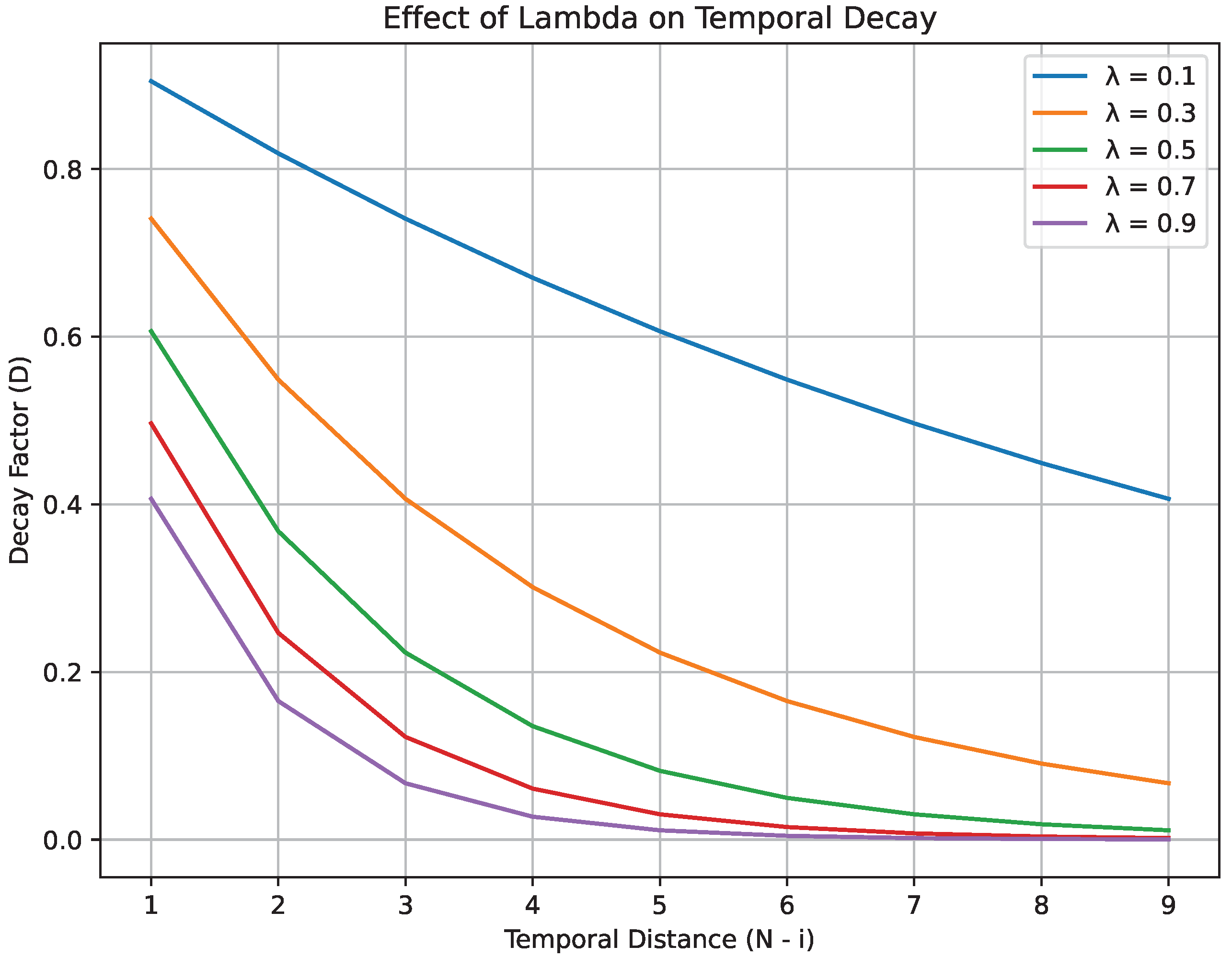
2.4. Exponential Decay Weighting

In this study, to improve the similarity vector produced by the SRW method, we propose a supplementary weight vector computation method that employs an exponential decay weighting scheme, which relies on the temporal distance between nodes. This idea is based on the intuitive assumption that nodes appearing later in the time series exhibit higher predictive significance compared with those appearing earlier. This approach mathematically determines the temporal decay factor assigned to each node, i, based on the temporal distance from the last node, N, which is represented as follows:

$$D_i=e^{-\lambda ·(N-i)},$$

(10)

where $\lambda >0$ controls the rate of decay and $N-i$ is the temporal distance between node i and the last node.

The parameter $\lambda$ in the exponential decay function determines how quickly the impact of older nodes decreases over time. For example, if $\lambda$ values are lower than 0.1, the decay process is gradual, allowing even the most outdated nodes to maintain a notable level of influence. Moreover, a balanced decay rate occurs when $\lambda$ takes values in the range of 0.1 to 0.5. In this case, the more recent nodes assert greater influence, but the older nodes also maintain their presence in the calculation. In contrast, when $\lambda$ exceeds 0.5, the decay is rapid and only the most recent nodes exert considerable influence on the prediction. Figure 1 demonstrates the manner in which varying $\lambda$ values influence the temporal decay factor.

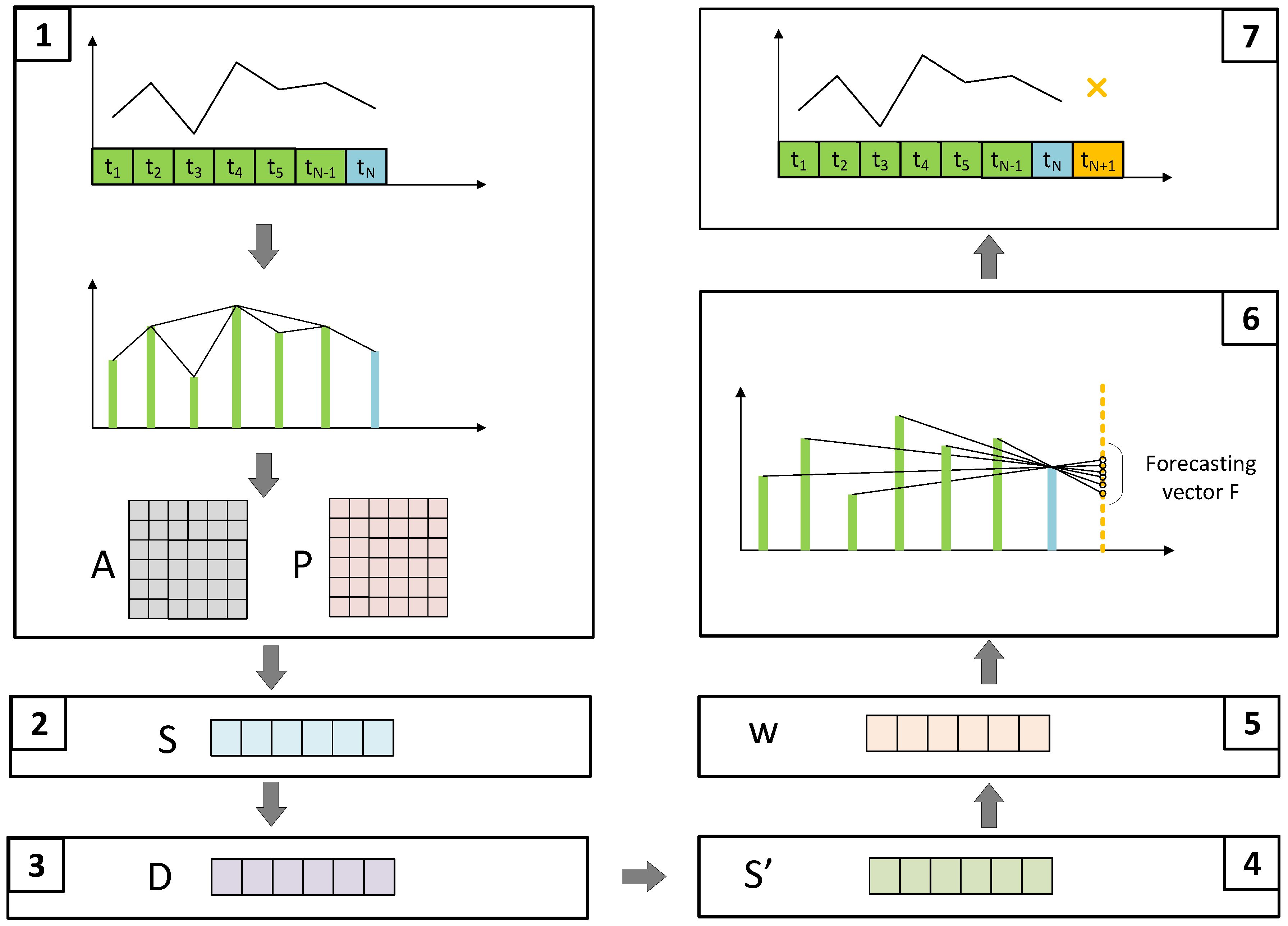
2.5. Forecasting Model

In this research, a weighted forecasting method is presented that combines visibility graphs, similarity vectors, and the notion of temporal decay. The visibility graph transforms time series data into a network, where each node represents a data point, and the edges are determined based on a pre-defined visibility criterion. Furthermore, a similarity vector is employed to measure the similarity between patterns within the time series, enhancing the predictive power of the model. By integrating these two components, the method provides a robust framework for accurate and insightful forecasting.

Our proposed model is an enhancement of previous research that incorporates advanced techniques to improve performance and accuracy.

The forecast methodology introduced, as illustrated in the seven phases in Figure 2, utilizes the proceeding phases for each variable in a multivariate time series, $X\left(t\right)$, to predict the value ${\widehat{y}}_{n+1}$ for the next time step:

• A time series is transformed into an undirected visibility graph, and the adjacency, A, and transition, P, matrices are computed.
• The similarity vector $S=[s_1,s_2,\dots ,s_{N-1}]$ is calculated using the SRW method.
• The temporal decay factor vector, D, is computed.
• An adjusted similarity vector, $S^{\prime }$, is calculated by combining the similarity vector, $S^{\prime }$, with the decay factor, D:

  $$S_i^{\prime }=S_i·D_i,\forall i\in [1,N-1],$$

  where $S_i^{\prime }$ is the adjusted similarity vector after applying the temporal decay.
• The adjusted similarity vector is normalized to form the weight vector, w:

  $$w_i={\displaystyle \frac{S_i^{\prime }}{{\sum }_{j=1}^{N-1}{S}_j^{\prime }}},\forall i\in [1,N-1]$$
  This normalized weight vector ensures that the total weight sums to 1.
• Each element, $\widehat{y_i}$, of the forecasting vector $F=[{\widehat{y}}_1,{\widehat{y}}_2,\dots ,{\widehat{y}}_{N-1}]$ is calculated based on the methodology proposed by Zhan and Xiao [39]. The $\widehat{y_i}$ is the predicted value by linear fitting vertex $t_i$ to the predicted vertex and is computed by the following equation:

  $${\widehat{y}}_i=y_N+{\displaystyle \frac{y_N-y_i}{t_N-t_i}}$$
• The weight vector, w, is used to compute the prediction for the next time step:

  $${\widehat{y}}_{n+1}=w·F$$

2.6. Comparison Models

In order to evaluate the accuracy of the results generated by the proposed methodology, the following models are used for comparison.

LightGBM (LGBM): Light Gradient Boosting Machine (LightGBM) is a distributed gradient-boosting framework created by Microsoft for machine learning. LGBM builds decision trees to find patterns in the data that grow by focusing on the most important parts first, making it a faster algorithm. LightGBM is suitable for classification, regression, and ranking tasks due to its parallelization that enables GPU processing.

ARIMA: the auto-regressive integrated moving average (ARIMA) is one of the variations of the auto-regressive moving average. It is a widely used technique for time series forecasting. It incorporates three elements: autoregression that looks at past values to predict future ones, differencing to stabilize the series by removing trends, and a moving average model to smooth out random fluctuations by averaging past errors.

Exponential smoothing (ES): Exponential smoothing is a forecasting method that assigns more weight to the most recent values and gradually decreases the weight for older values. It smooths out short-term fluctuations and highlights longer-term trends.

CNN-LSTM: The Convolutional Neural Network (CNN) and Long Short-Term Memory network (LSTM) is a hybrid deep learning model that leverages the strengths of both architectures. CNNs are powerful at automatically extracting spatial features from input data, typically used for image processing tasks due to their ability to recognize patterns and structures. LSTMs, a type of recurrent neural network (RNN), are designed to capture and learn temporal dependencies due to their memory cell capabilities, making them effective for sequence prediction. By integrating CNNs and LSTMs, the hybrid model can simultaneously handle complex spatial and sequential patterns, which is particularly beneficial in applications like video analysis, where both spatial and temporal features are critical for accurate predictions and classifications.

3. Experiments

In this section, the data set is described, together with an analysis of its characteristics and features. Following the description of the data set, the prediction performance is evaluated using various error metrics. The software environment and experimental setup are described to ensure reproducibility. The experimental results highlight and detail key findings.

3.1. Data Set Description

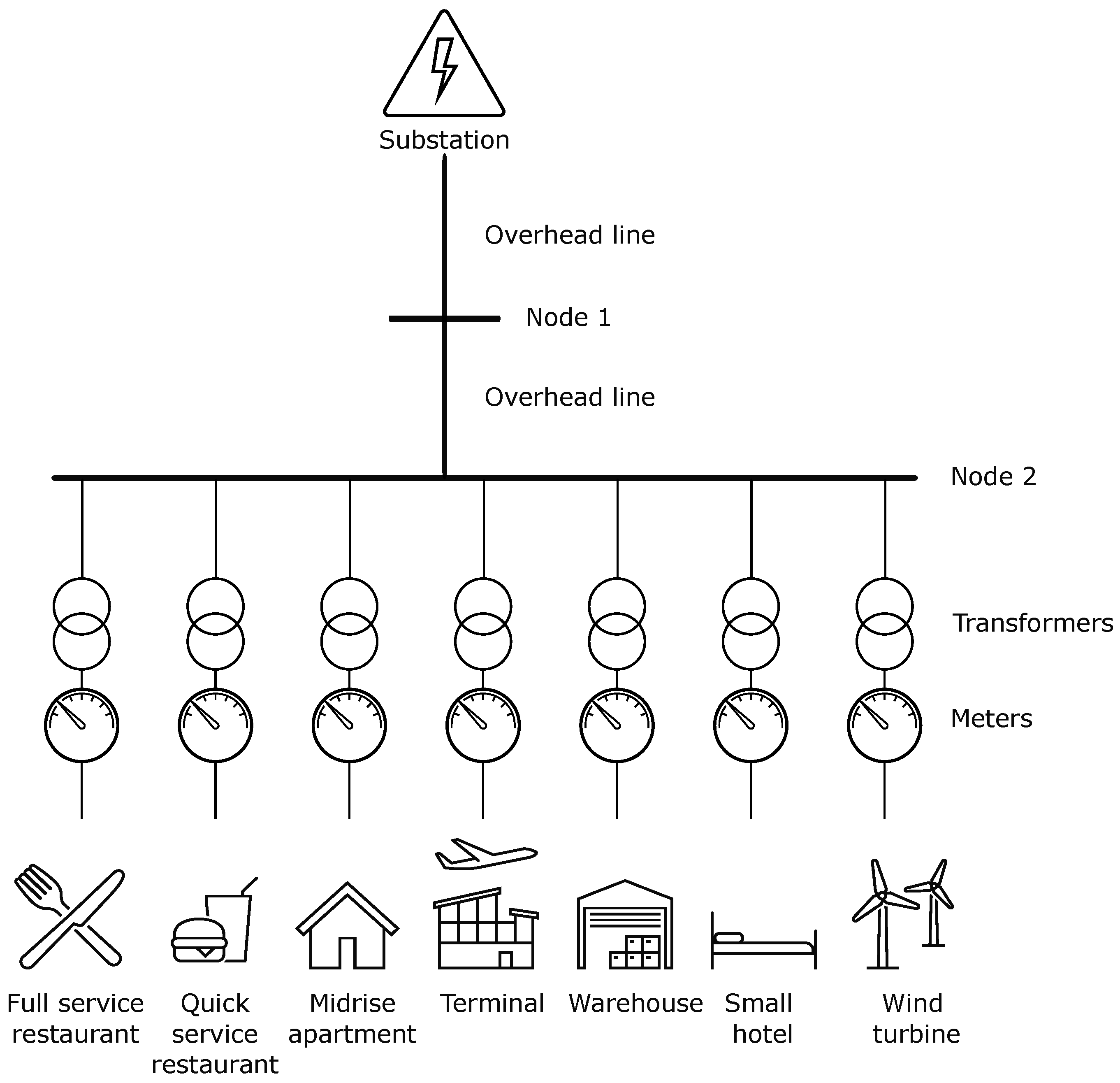
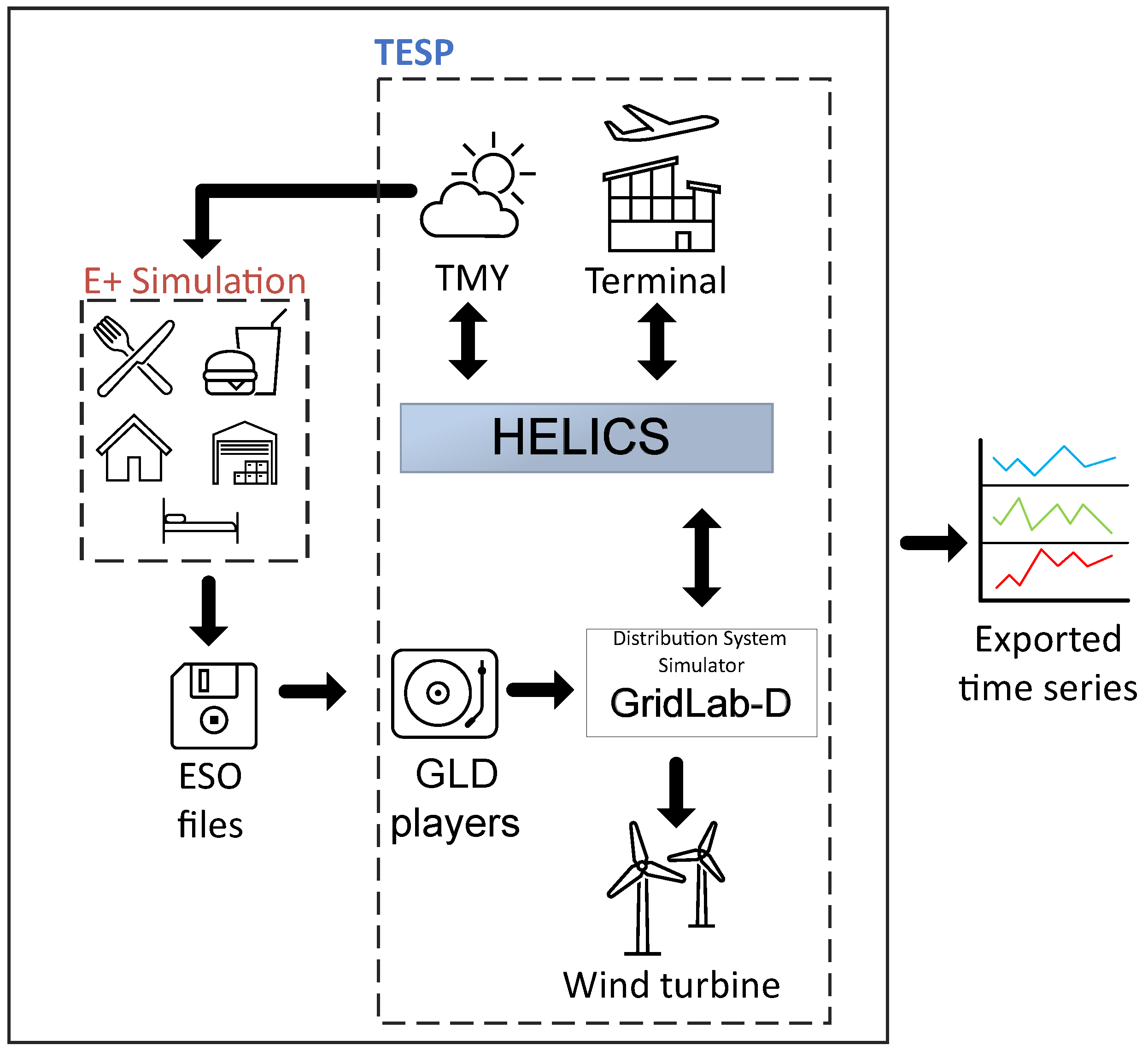
The data set analyzed in this paper is generated using the TESP simulation software, which integrates EnergyPlus (E+) for building simulation, GridLAB-D (GLD) for simulation and modeling of distribution energy systems, and HELICS for co-simulation of energy systems. This synthetic data set represents the energy dynamics of a regional airport in Greece, which includes data on power consumption from various types of buildings, as well as the power production from renewable sources. The use of TESP ensures high fidelity in representing both building-specific energy demands and renewable energy contributions, simulating real-world interactions between the built environment and power systems. This data set offers insights into the interaction of different energy profiles in buildings and renewable energy generation, making it a reliable platform to explore energy optimization, demand response strategies, and sustainability measures in airport settings.

More specifically, the distribution energy system is modeled by GLD and consists of a substation, a GLD object for TESP power metrics, and serves six buildings and a wind turbine that are connected to node 2, as illustrated in Figure 3. The terminal building is modeled with E+ and co-simulated in GLD. The design of the terminal is extensively described in the previous work of the researchers [12,41]. Additionally, the warehouse, full service restaurant, quick service restaurant, small hotel, and midrise apartment buildings are E+ prototype building models [42], which were simulated individually, and the E+ variable of the generated eso file “Facility Total Electric Demand Power” is exported per time step. Subsequently, a GLD player is instantiated for each building, providing phase-specific power input to the GLD model. The flight information fed into the terminal model and the weather conditions for the generation of a Typical Meteorological Year (TMY3) file are used for the Greek island of Santorini for 2018. The simulation period is from 1st of April to 31th of October, a typical tourist season for a Greek island, with a simulation duration of 5148 h and a 30 min time step (2 time steps per hour). It should be noted that the initial data set did not exhibit problematic values, thereby eliminating the need for additional preprocessing. Figure 4 illustrates the simulation procedure described above.

3.2. Data Set Analysis

The data set analysis section is structured into three distinct parts: statistical analysis, stationarity analysis, and dynamics analysis, each providing a comprehensive examination of the characteristics and behavior of the data.

3.2.1. Statistical Analysis

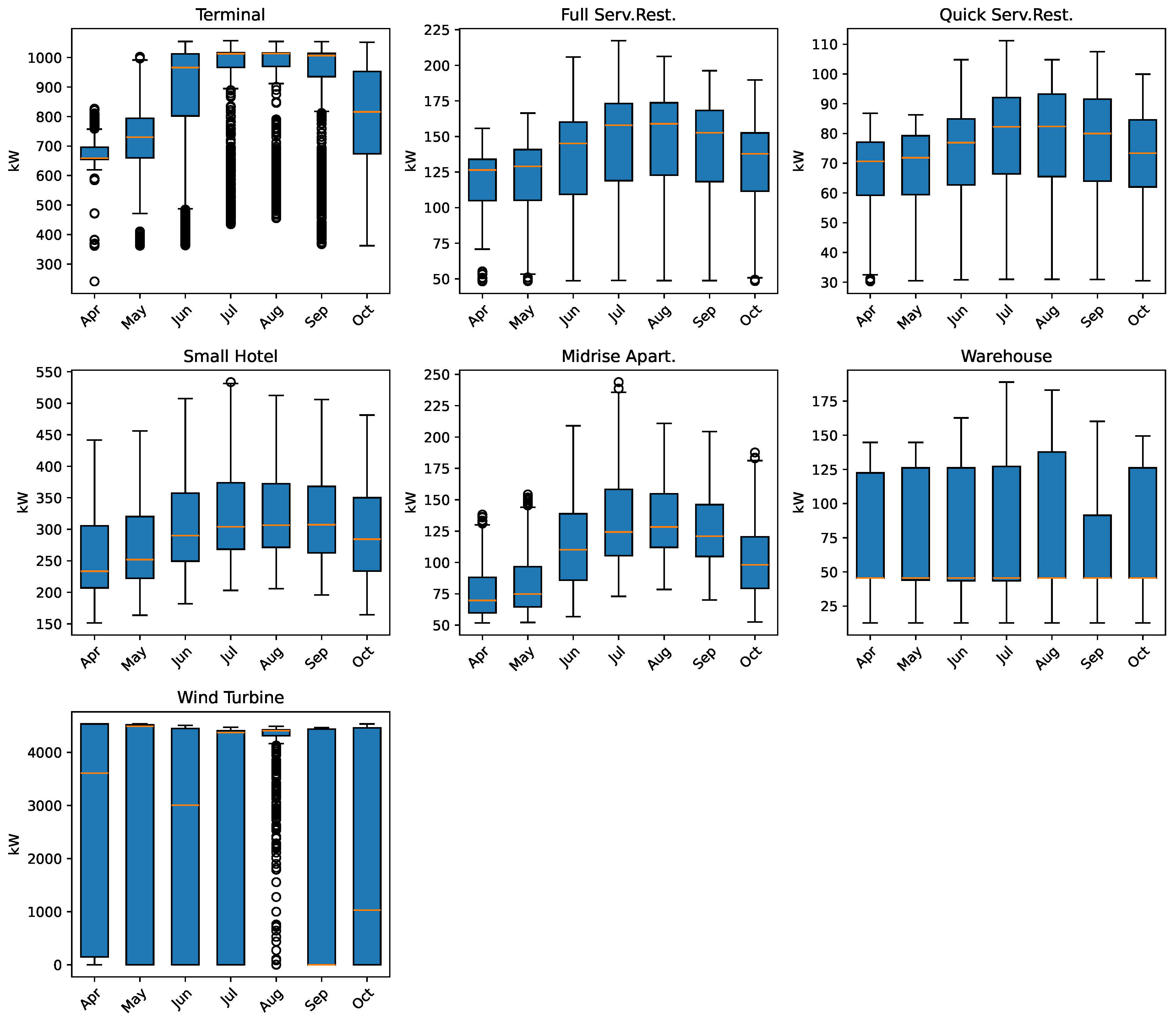
In this section, a comprehensive statistical analysis of the time series data is provided. Figure 5 illustrates box plots for each time series in all months of the data set, which visually depict the central tendency, dispersion, and potential outliers within the data. Furthermore,

Table 1. Statistical values.

Month	Variable	Min	Max	Std Dev	Variance
	Terminal	241.13	826.51	116.47	13,564,604.81
	Full Serv.Rest.	48.15	155.72	31.84	1,013,929.60
	Quick Serv.Rest.	30.25	86.79	17.53	307,211.76
April	Small Hotel	151.45	441.65	74.21	5,507,438.88
	Midrise Apart.	51.75	138.15	21.40	457,957.61
	Warehouse	12.66	144.76	46.12	2,127,365.08
	Wind Turbine	0.00	4537.02	1942.89	3,774,836,614.66
	Terminal	434.95	1057.39	164.14	26,940,590.26
	Full Serv.Rest.	48.78	217.37	47.90	2,294,694.27
	Quick Serv.Rest.	30.97	111.23	23.39	547,280.80
July	Small Hotel	203.05	533.51	77.89	6,067,212.51
	Midrise Apart.	72.92	243.83	35.50	1,259,984.16
	Warehouse	12.66	188.90	52.09	2,713,143.78
	Wind Turbine	0.00	4473.43	2080.26	4,327,460,907.98

presents the minimum, maximum, standard deviation, and variance measures for each time series to provide information about the months April and July, which are the months that present the lowest and maximum dispersion values in the data set, respectively.

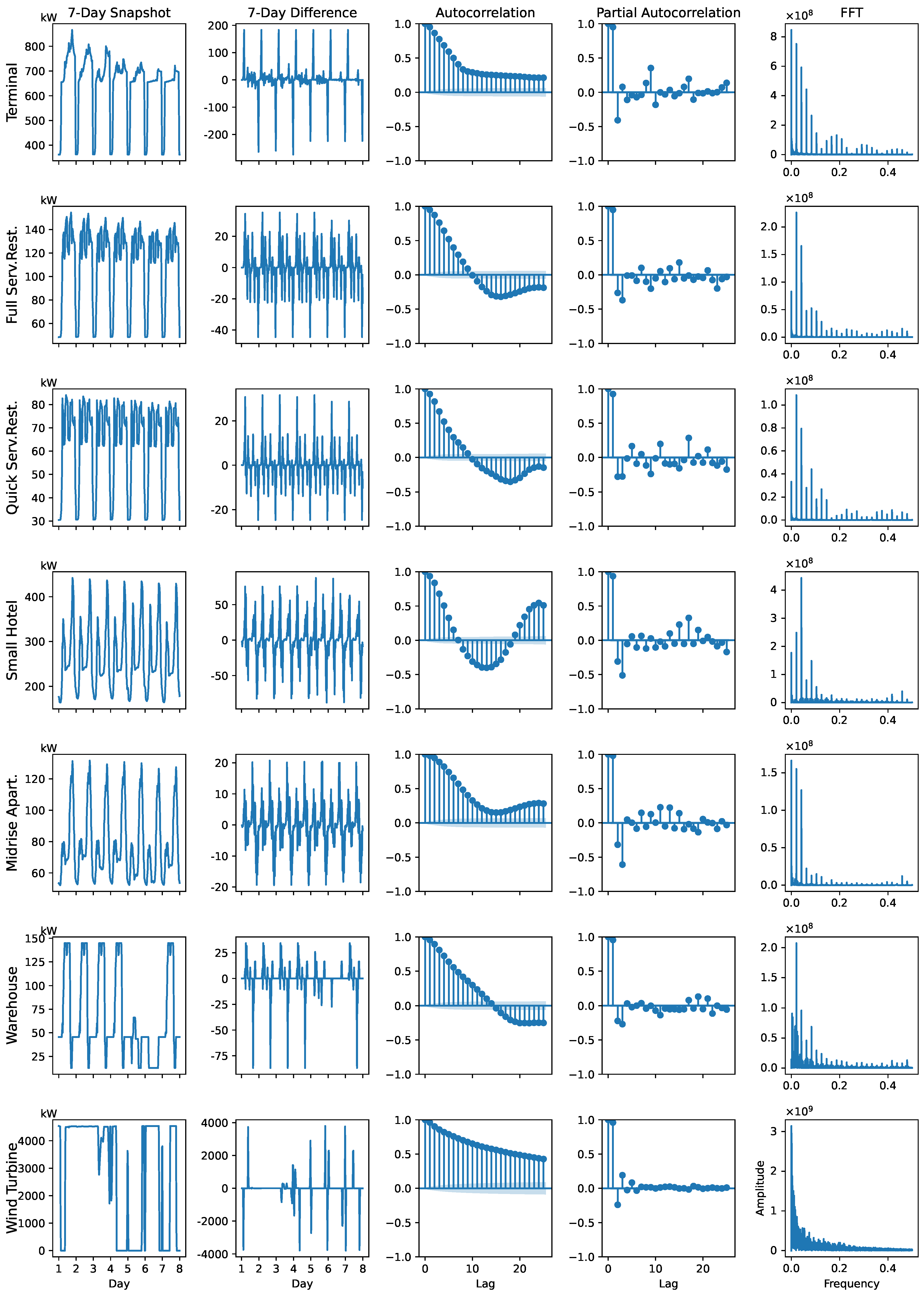
Figure 6 provides a detailed visualization of the energy consumption patterns in different categories, highlighting their temporal characteristics. The first column shows the original time series over a 7-day period, revealing distinct patterns such as daily periodicity and seasonality in most cases, especially for the terminal, full service restaurant, quick service restaurant, small hotel, and midrise apartment. In contrast, the warehouse and wind turbine exhibit irregular and erratic behavior with no consistent cycles.

The second column illustrates the first-order difference series, which effectively removes trends and enhances the focus on shorter-term fluctuations. For the categories with clear periodicity in the original series, this transformation results in stabilized fluctuations, indicating more consistent short-term patterns. However, for the warehouse and wind turbine, the differencing does not eliminate the erratic nature of the fluctuations, suggesting the persistence of irregular behavior.

The third and fourth columns present autocorrelation and partial autocorrelation plots, offering insights into how the values in each time series are related over different time lags. Series such as terminal, full service restaurant, quick service restaurant, small hotel, and midrise apartment show a gradual decay in autocorrelation, reflecting the presence of strong seasonal cycles in the original series. On the other hand, the warehouse and wind turbine display persistent or erratic autocorrelation patterns, indicating less predictable behavior.

The final column displays the frequency domain analysis using fast Fourier transform (FFT), which reveals the dominant frequencies in the series. Strong peaks are evident for series with clear periodicity, such as daily cycles, confirming the influence of recurring patterns. However, for the warehouse and wind turbine, the FFT plots lack dominant frequencies, further emphasizing their irregular and unpredictable nature. In general, the visualizations in Figure 6 highlight different temporal behaviors, with certain series exhibiting well-defined periodic characteristics and others marked by irregular variability.

3.2.2. Stationary Analysis

To assess the stationarity of the time series in this study, a number of unit root tests are executed, as described below. The Augmented Dickey–Fuller (ADF) and Kwiatkowski–Phillips–Schmidt–Shin (KPSS) tests are applied to raw and differenced data. In addition, the Dickey–Fuller GLS test (DFGLS), an enhanced ADF test, is used [43]. This test applies GLS-detrending before the ADF regression without extra deterministic terms. The ADF and DFGLS tests assume that the null hypothesis, $H_0$, implies a unit root, and the alternative hypothesis, $H_A$, implies no unit root. A p-value less than 0.05 leads to rejection of $H_0$, indicating stationarity. Conversely, the KPSS test posits $H_0$ as a non-unit root. In the KPSS test, p-values range from 0.01 to 0.1; values outside this range are not provided.

Table 2. Results of the conducted unit root tests.

Series	KPSS	ADF	KPSS-Diff	ADF-Diff	DFGLS
Terminal	0.01	0	0.10	0	0.498
Full Serv.Rest.	0.01	0	0.10	0	0.570
Quick Serv.Rest.	0.01	0	0.10	0	0.589
Small Hotel	0.01	0	0.10	0	0.631
Midrise Apart.	0.01	0.0937	0.10	0	0.136
Warehouse	0.10	0	0.10	0	0
Wind Turbine	0.10	0	0.10	0	0

shows that the warehouse and wind turbine series are stationary, while the others possess a unit root, corroborating the statistical analysis findings.

3.2.3. Dynamics Analysis

A time series dynamics analysis is performed in order to select the value of the decay rate, $\lambda$, according to Algorithm 1. The algorithm evaluates each time series to recommend the best lambda value for dynamic modeling. It starts by normalizing the series to eliminate scale effects, and then calculates the autocorrelation function (ACF) to evaluate temporal dependencies. The delay in lowering the ACF below a set threshold is identified, indicating the decay rate of the autocorrelation. Based on these findings, the algorithm proposes a lambda: higher for variable series and lower for stable ones. This ensures that the lambda mirrors both the temporal structure and the variability, which are suitable for adaptive modeling.

Algorithm 1 Analyze Time Series for Lambda

Require:  Time series data $time\_series$ Ensure:  Suggested $\lambda$ value Normalize the time series: $$normalized\_series\leftarrow {\displaystyle \frac{time\_series-\mathrm{mean}(time\_series)}{\mathrm{std}(time\_series)}}$$ Compute the autocorrelation function (ACF): $$acf\_values\leftarrow \mathrm{ACF}(normalized\_series,\mathrm{lags}=40)$$ Measure the rate of autocorrelation decay: $$decay\_threshold\leftarrow 0.4$$ $$lag\_decay\leftarrow min\left\{lag\right||acf\_values[lag\left]\right|<decay\_threshold\}$$ Suggest $\lambda$ based on autocorrelation decay: if  $lag\_decay<5$  then   $\lambda \_suggestion\leftarrow 0.5$ else if  $5\le lag\_decay\le 15$  then   $\lambda \_suggestion\leftarrow 0.2$ else   $\lambda \_suggestion\leftarrow 0.1$ end if    return  $\lambda \_suggestion$

3.3. Evaluation of the Predictions

The performance of each model is evaluated by the following metrics: mean absolute error in kW (MAE), symmetric mean absolute percentage error in percentage (SMAPE), normalized root mean square error (NRMSE) and R-squared ($R^2$), which are metrics utilized in power prediction tasks.

$$\mathrm{MAE}={\displaystyle \frac{1}{n}}\sum _{i=1}^n|y_i-{\widehat{y}}_i|$$

(11)

$$\mathrm{SMAPE}={\displaystyle \frac{100\%}{n}}\sum _{i=1}^n{\displaystyle \frac{|{\widehat{y}}_i-y_i|}{\left(\right|y_i|+|{\widehat{y}}_i\left|\right)/2}}$$

(12)

$$\mathrm{NRMSE}={\displaystyle \frac{\sqrt{\frac{1}{n}{\sum }_{i=1}^n{(y_i-{\widehat{y}}_i)}^2}}{\overline{y}}}$$

(13)

$$R^2=1-{\displaystyle \frac{{\sum }_{i=1}^n{(y_i-{\widehat{y}}_i)}^2}{{\sum }_{i=1}^n{(y_i-\overline{y})}^2}}$$

(14)

where, $y_i$ denotes the actual values, $\overline{y}$ is the mean of $y_i$ values, ${\widehat{y}}_i$ represents the predicted values, and n represents the observed samples.

MAE measures the average magnitude of errors in a set of predictions, expressed as an average of absolute differences between predicted and actual values, with a range starting from 0, where lower values indicate better predictions. SMAPE, on the other hand, is used to measure the accuracy of forecasts by comparing the absolute difference between forecasts and actuals with their mean, with values typically ranging from 0% to 200%. NRMSE is a normalization of the root mean square error by dividing it by the mean of the observed data, providing a relative measure of prediction accuracy, with values starting from 0, where lower values signify fewer errors. Finally, R-squared indicates the proportion of variance in the dependent variable that is predictable from the independent variables, ranging from $-\infty$ to 1, with values closer to 1 representing a better fit of the model to the data [44].

3.4. Software Environment and Experimental Setup

These research experiments were conducted on the Google Colab Platform with Python 3 Google Compute Engine backend, which utilizes an Intel Xeon CPU with two virtual CPUs, system RAM 12.7 GB, and available disk space 107.7 GB. Python 3.10 programming language was used for the code development with the incorporation of Python Pandas 2.1.0 and Numpy 1.26.0 libraries for data analysis, Seaborn 0.13.0, and Matplotlib 3.9.0 for visualization purposes of exploratory analysis and predicted results. Additionally, the NetworkX Python library was used for graph analysis, while the statsmodels, arch, and scipy libraries were utilized for the stationary and dynamics analysis of the data set. Moreover, the libraries statsforecast and mlforecast were applied for the comparison models.

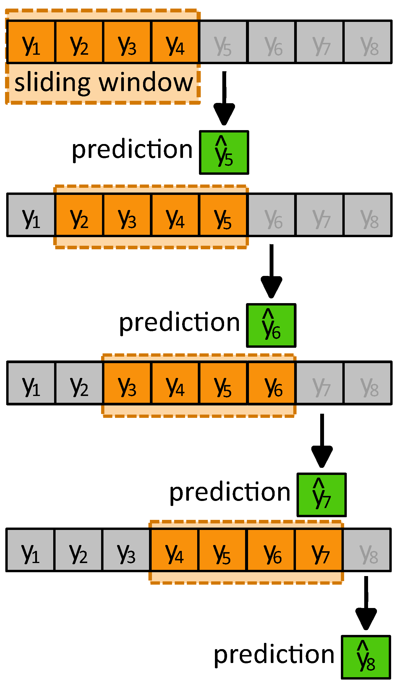
The proposed forecasting method is applied as a monthly prediction. A predetermined number of time steps are chosen as the retained data. The expression “retained data” refers to a set of previous true values used for the projection of the future value. During each prediction phase, the retained data set is updated using the sliding window method by adding the next actual value. This adjustment, implemented by the prediction algorithm, estimates the value of the subsequent step, as shown in Figure 7.

In this application, the first 48 time steps (1 day) are taken as the retained data set, and the prediction starts from the first time step of the second day. Additionally, following the analysis of time series dynamics, the value of the decay rate, $\lambda$, is selected as 0.2 for the entire time series. For the sake of clarity in presenting the results, we limit our illustrations to the months of April and July, which present different value fluctuations resulting from the data set analysis. Given the software configuration and the sliding window approach used, predicting each monthly time series takes around 8 min. In contrast, more advanced prediction algorithms demand more powerful computational resources for time-intensive tasks such as hyperparameter tuning and model training.

3.5. Experimental Results

In this section, the experimental results are presented comparing the proposed method with the baseline models: LGBM, ARIMA, ES, and CNN-LSTM, which are evaluated by the metrics mentioned above. The results are detailed in

Table 3. Experimental results.

		April				July
		MAE	SMAPE (%)	NMRSE (%)	${\mathit{R}}^{\mathbf{2}}$	MAE	SMAPE (%)	NMRSE (%)	${\mathit{R}}^{\mathbf{2}}$
Terminal	LGBM	13.13	2.01	3.86	0.96	40.32	4.55	6.13	0.87
	ARIMA	18.44	2.96	3.97	0.95	29.25	3.81	4.54	0.93
	ES	10.43	1.49	4.12	0.95	48.75	6.56	7.09	0.83
	CNN-LSTM	71.56	12.68	13.88	0.45	53.52	6.82	9.07	0.72
	proposed	25.43	5.32	7.68	0.83	34.3	4.82	7.4	0.82
Full Serv.Rest.	LGBM	8.17	8.58	9.72	0.89	33.81	32.26	27.61	0.34
	ARIMA	1.24	1.01	2.35	0.99	18.18	14.11	15.3	0.8
	ES	1.25	1.02	2.39	0.99	12.17	7.97	10.88	0.9
	CNN-LSTM	7.03	7.44	9.18	0.9	9.34	7.96	9.29	0.93
	proposed	9.22	10.03	11.84	0.83	10.92	10.8	10.49	0.9
Quick Serv.Rest.	LGBM	3.91	7.26	9.13	0.89	7.01	9.37	11.43	0.87
	ARIMA	0.46	0.7	1.55	1.0	6.14	8.02	10.21	0.89
	ES	0.46	0.7	1.56	1.0	5.15	6.33	8.88	0.92
	CNN-LSTM	4.61	7.95	10.22	0.86	5.76	8.39	10.0	0.90
	proposed	5.67	9.76	13.33	0.77	5.92	9.6	11.28	0.87
Small Hotel	LGBM	56.12	20.28	25.27	0.23	99.4	26.01	36.72	−
	ARIMA	10.11	3.88	6.86	0.94	35.92	10.7	13.35	0.69
	ES	10.29	3.96	6.93	0.94	20.29	6.46	8.21	0.88
	CNN-LSTM	19.73	7.36	10.23	0.87	20.21	5.96	8.31	0.88
	proposed	20.59	7.85	11.42	0.84	19.7	5.94	8.8	0.87
Midrise Apart.	LGBM	3.22	4.34	6.32	0.95	116.83	133.6	100.05	−
	ARIMA	3.09	4.15	6.34	0.95	57.43	60.57	49.17	−
	ES	2.56	3.4	6.1	0.95	21.81	17.91	19.07	0.45
	CNN-LSTM	5.26	6.64	8.92	0.9	6.25	4.8	6.14	0.94
	proposed	5.23	6.69	9.25	0.89	5.25	4.04	5.43	0.96
Warehouse	LGBM	16.22	22.69	60.61	0.22	371.92	139.05	629.62	−
	ARIMA	15.3	21.04	60.01	0.24	35.7	52.51	83.17	−
	ES	15.36	21.17	59.91	0.24	35.4	49.31	86.71	−
	CNN-LSTM	9.51	18.66	20.83	0.91	5.59	11.81	13.58	0.97
	proposed	7.46	21.06	22.84	0.89	7.44	22.68	23.77	0.9
Wind Turbine	LGBM	11,889.8	139.53	496.11	−	6940.3	198.94	275.49	−
	ARIMA	1793.93	77.33	87.53	−	2786.0	185.84	116.45	−
	ES	1849.73	75.38	97.89	−	2832.95	0.0	119.97	−
	CNN-LSTM	965.05	73.14	50.03	0.53	2649.56	180.23	113.66	−
	proposed	323.21	63.63	30.41	0.83	160.04	0.0	22.04	0.93

$R^2$ values represented by “−” indicate negative values.

, highlighting the effectiveness of our approach, in certain series, relative to the other models.

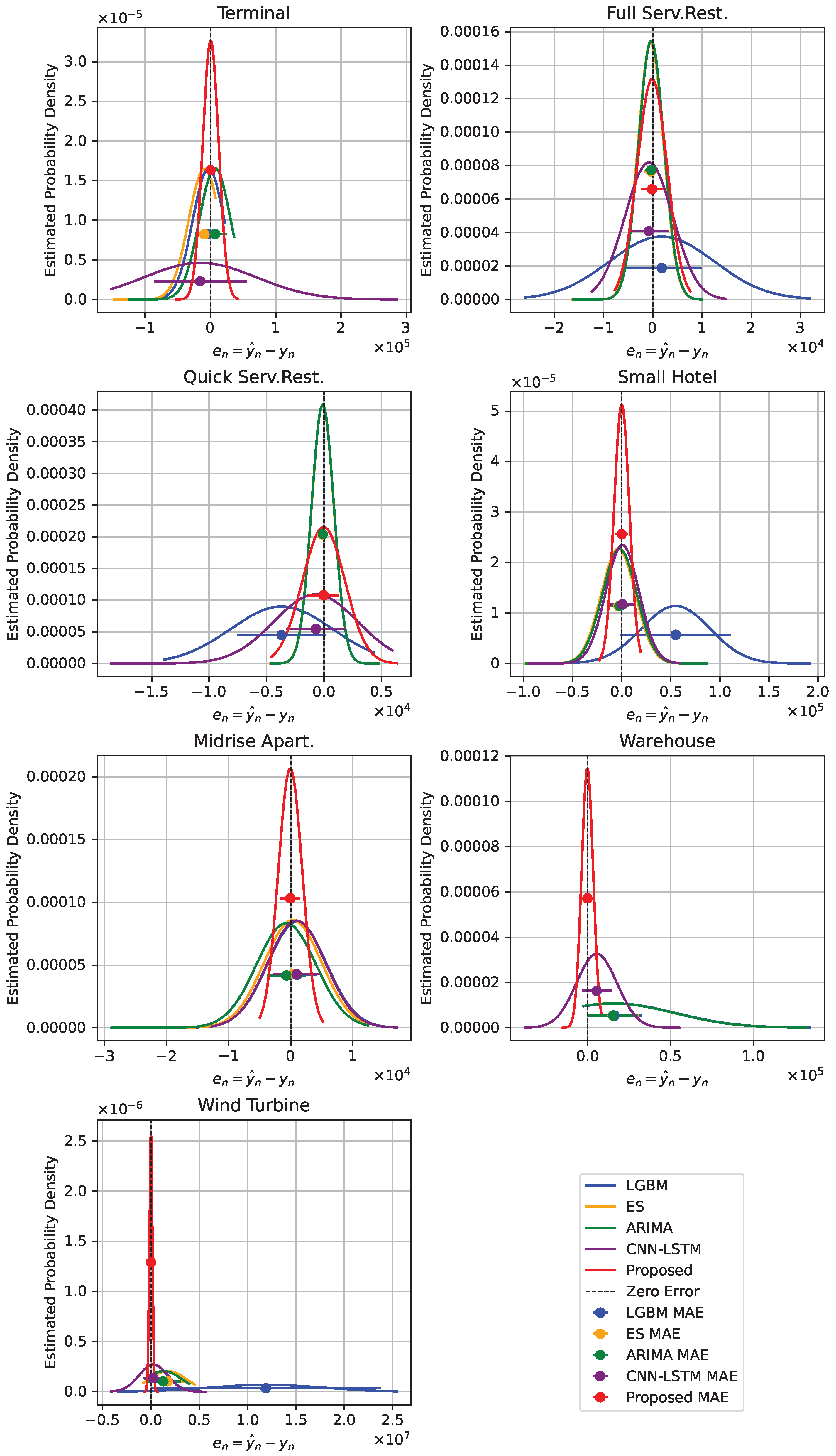
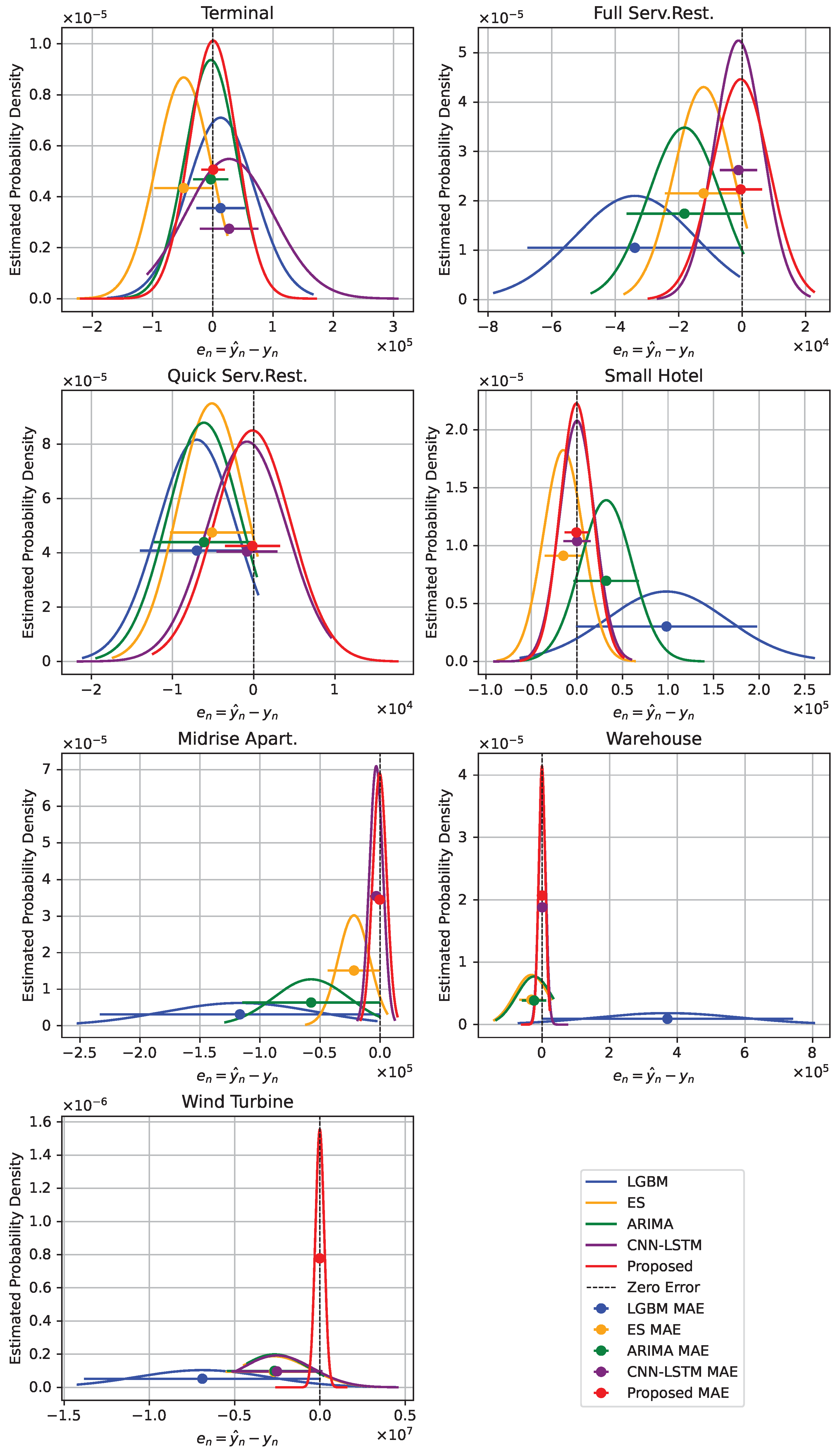
Furthermore, Figure 8 provides a comparative analysis between the outcomes proposed in the study and the actual data gathered for the months of April and July. Figure 9 and Figure 10 provide visual representations of probability density plots, which are used to compare the error distributions of the newly proposed model against those of the established baseline models. This comparison is specifically made for microgrid items over the periods corresponding to the months of April and July.

4. Discussion

This research offers an extensive assessment of the suggested method by comparing it with well-established models, including Exponential smoothing, ARIMA, LGBM, and CNN-LSTM. The evaluation is carried out across a diverse array of time series data, each displaying distinct characteristics. The suggested forecasting model shows satisfactory performance compared with other related methods. Although the proposed methodology is effective in many time series in July, it exhibits higher error rates in certain series in April compared with baseline models. In specific cases, the performance of the proposed approach lags behind other models, as evidenced by higher MAE, SMAPE, and NMRSE values. Despite its strengths, the proposed method shows limitations in data sets that present a smaller variability, where alternative methods perform better.

One of the key contributions of the proposed model is its robustness across varied building types and energy usage profiles. While methods like ES excel in specific domains, the proposed method maintains relatively consistent performance, avoiding the extreme variability observed in LGBM for categories like the wind turbine and midrise apartment, where LGBM shows large errors and negative $R^2$ values. The proposed model’s performance in wind turbine for instance is noteworthy, as it significantly reduces MAE and SMAPE compared with LGBM, demonstrating its suitability for scenarios involving complex energy usage patterns. More specifically, the perfect alignment of the forecasted time series with the actual values is remarkable, both for the terminal and the wind turbine, for time steps 200–240 in the month of April. No oscillations are observed in the predictions, as is the case with comparable deep learning models, which further strengthens the performance of the proposed model. The results of the proposed model demonstrate robustness and stability in terms of prediction accuracy. This is further reinforced by the small hotel curves, where the fluctuations of the predicted and actual values are almost identical for April.

In addition, its $R^2$ values across categories suggest that the proposed model explains a substantial proportion of variance in energy consumption, offering a balance between accuracy and generalization. In particular for wind turbine forecasts conducted in July, all the comparative models display negative values, suggesting a tendency to underpredict the actual observed values. Moreover, the proposed method demonstrates a remarkable capacity to preserve high performance across various seasons, as evidenced by the data collected in April and July. This observation underscores its resilience to temporal fluctuations, which is of paramount importance for applications involving long-term forecasting. In such contexts, the variations due to different seasons can have a significant effect on the accuracy of predictions. Also, compared with the hybrid CNN-LSTM model, it is observed that in the cases of the terminal, midrise apartment, warehouse, and wind turbine, our proposed model exhibits a lower MAE. This is quite promising, as hybrid models are generally considered to be more powerful than single models most of the time.

Furthermore, Figure 9 and Figure 10 depict the error distribution plots, which effectively showcase the relative performance of the proposed methodology, consistently exhibiting superior accuracy and robustness in comparison with other methods. It is important to note that the suggested approach consistently demonstrates error forecasting distributions that are more tightly clustered around the zero-error line. This observation suggests that the prediction capability of our proposed methodology is more reliable when applied to various time series data sets, especially when compared with established baseline models. In particular, for complex elements like the wind turbine, the proposed method exhibits enhanced performance, demonstrating its robustness and dependability in varied contexts. These outcomes underscore the proposed method’s effectiveness in delivering more accurate and consistent forecasts.

Some challenges still need further exploration. Converting large time series into visibility graphs and adjusting similarity vectors based on decay can be computationally demanding, which might make real-time use difficult. Additionally, the effectiveness of the method across different data sets relies on the quality of the input data. Future research should focus on improving its efficiency and testing its performance in real-time forecasting situations.

The findings show that this approach has strong potential for energy forecasting in microgrids. While there are some limitations in minimizing error rates, the model remains a reliable and flexible tool for predictions. Future work could refine its accuracy by combining it with other techniques or fine-tuning its parameters to make it more competitive, especially for fast-changing data like those from the quick service restaurant and terminal. Moreover, this forecasting model could be applied to the task of multistep prediction. By improving its methodology, this model could become a valuable tool for predicting energy demand in different types of buildings.

5. Conclusions and Future Directions

This study presents a new approach to load forecasting that uses visibility graph transformations, the SRW method, and temporal decay adjustments to predict future energy demand. The method was tested in a microgrid at a regional airport, which includes multiple buildings with different patterns of energy use and a renewable energy source.

The results show that the proposed forecasting model exhibits satisfactory performance relative to comparison models, such as Exponential smoothing, ARIMA, Light Gradient Boosting Machine, and CNN-LSTM, while it performs reasonably well in various types of buildings and energy consumption patterns. The proposed method shows improved performance in forecasting energy consumption for both stationary and highly variable time series, with SMAPE and NMRSE values typically in the range of 4–10% and 5–20%, respectively, and an $R^2$ reaching 0.96. It provides a flexible tool for predicting energy demand in different structures and energy production systems within a microgrid.

In our approach, the SRW method improves the accuracy of the prediction by adjusting the influence of past observations on the forecast, and temporal decay adjustments give more weight to recent data, making it easier to respond to changing demand. Together, these techniques create a forecasting model that works well for different types of building and scenarios of energy consumption. Moreover, unlike many deep learning models, it avoids issues such as overfitting and high computational demands, making it a practical option for forecasting tasks. More generally, this method introduces a new way of forecasting time series data by combining graph theory, temporal decay, and similarity-based weighting. Its flexibility makes it useful for a wide range of applications, including power systems, finance, and environmental science.

Regarding future research directions, the proposed model should aim to build on the current methodology by testing its performance across a wider variety of scenarios and data sets. One promising direction is to incorporate additional external variables, such as weather conditions, occupancy data, and economic indicators, to further improve the accuracy of the prediction. Also, alternative weighting schemes for the temporal decay adjustment must be studied, allowing for a more dynamic response to shifts in demand patterns. Moreover, to further bolster the robustness of our proposed model, it is essential to conduct comparisons with other sophisticated hybrid approaches and data-driven methods that extend beyond traditional machine and deep learning methodologies. Additionally, incorporating supplementary features or employing hybrid modeling approaches could further augment the model’s performance, especially when dealing with data sets characterized by significant seasonal variability. Another noteworthy case is the integration of our own proposed model into hybrid and ensemble advanced models, aiming to further enhance its performance and create even more novel algorithms.

Furthermore, extending the evaluation to other industries and longer time frames would provide a more holistic understanding of the model’s capabilities and limitations. Moreover, performing a sensitivity analysis on the parameters of the visibility graph transformations and the SRW method may uncover opportunities for fine-tuning the model. In addition, application of the approach in real-time microgrid environments and integration with other advanced forecasting techniques could provide valuable insights into its scalability and operational robustness in practical settings. It is anticipated that further comparison of the model proposed here with other models and simulations in related studies will stimulate scientific interest in this field and promote research efforts in this area.