Article

Effect of Battery Degradation on the Probabilistic Optimal Operation of Renewable-Based Microgrids

by
Mahshid Javidsharifi
1,*,
Hamoun Pourroshanfekr Arabani
2,
Tamas Kerekes
1,
Dezso Sera
3,
Sergiu Spataru
4 and
Josep M. Guerrero
1
1
Department of AAU Energy, Aalborg University, 9220 Aalborg, Denmark
2
Division of Industrial Electrical Engineering and Automation, Lund University, SE-22100 Lund, Sweden
3
Faculty of Science and Engineering, Queensland University of Technology, Brisbane, QLD 4000, Australia
4
Department of Photonics Engineering, Technical University of Denmark, 4000 Roskilde, Denmark
*
Author to whom correspondence should be addressed.
Electricity 2022, 3(1), 53-74; https://doi.org/10.3390/electricity3010005
Submission received: 16 November 2021 / Revised: 26 December 2021 / Accepted: 6 January 2022 / Published: 4 February 2022
(This article belongs to the Special Issue Recent Advances in Energy Storage Systems)

Abstract

:
In order to maximize the use of renewable-based distributed generators (DGs), in addition to dealing with the effects of the inherent power management uncertainties of microgrids (MGs), applying storage devices is essential in the electrical system. The main goal of this paper is to minimize the total operation cost as well as the emissions of MG energy resources, alongside the better utilization of renewable energy sources (RES) and energy storage systems. The uncertainties of wind speed, solar irradiation, market price and electrical load demand are modeled using reduced unscented transformation (RUT) method. Simulation results reveal that, as expected, by increasing the battery efficiency, the achievable minimum daily operational cost of the system is reduced. For example, with 93% battery efficiency, the operational cost equals EUR 9200, while for an efficiency of 97%, the achievable minimum daily operational cost is EUR 8900. Moreover, the proper economic/environmental performance of the suggested approach, which contributes to the possibility of selecting a compromise solution for the MG operator in accordance with technical and economic constraints, is justified.

1. Introduction

In order to fulfill the increasing energy demand and to mitigate the environmental concerns related to energy generation from fossil fuels, the development of RESs has been expedited [1,2,3,4,5]. MGs, as an aggregation of DERs and loads with distribution networks, were presented to provide three main advantageous features, including reliability, sustainability and cost-effectiveness [1]. DERs include both renewable (such as PV systems and WTs) and non-renewable technologies (such as micro-turbines and diesel generators). RESs attracted much attention owing to their availability and sustainability. However, their inherent uncertainties raise new challenges [2]. These challenges, however, can be resolved by combining energy storage devices to RESs in MGs [2]. Energy storage devices, such as batteries, play an important role in the stability, reliability and performance of renewable-based MGs [1,2,3,4,5]. A review of different storage technologies and some major storage devices that are used in MGs were deliberated in [3,4], respectively.
The multi-objective probabilistic economic/emission optimal operation of renewable-based MGs is considered in this paper. A variety of methodologies were suggested in the literature to solve the multi-objective problems related to energy systems, including programming-based optimization approaches and meta-heuristic algorithms [5]. However, the two main reasons that make meta-heuristic algorithms more suitable than mathematical programming approaches for solving multi-objective optimization problems are listed as follows [5]:
  • Meta-heuristic algorithms deal simultaneously with a set of feasible solutions; this allows different solutions to be found in the Pareto optimal front in just one execution of the algorithm. While in the mathematical programming approaches, a sequence of independent executions should be dealt with.
  • Meta-heuristic algorithms are not sensitive to the continuity and formation of the Pareto front, which is one of the drawbacks of mathematical programming.
Research was conducted that dealt with the optimal operation management of MGs, considering different constraints and objectives. Some papers focused on conventional economic dispatch [6,7], while some studied the scheduling of energy storage systems [8]. Soares et al. [9] proposed a “signaled particle swarm optimization” for MG scheduling. A day-ahead MG scheduling problem was considered in [10], using a hybrid harmony search algorithm with differential evolution. The authors of [11] proposed a robust optimization-based method for solving optimal MG management problems. Elsied et al. [12] applied a binary PSO to optimize MG performance in real-time operations, where the objectives were to minimize the energy cost, carbon dioxide and pollutant emissions, while maximizing the power of the available RESs. In [13], a “real-time energy management system” was introduced to take the advantage of GA for minimizing energy costs and carbon dioxide emissions, while maximizing the power of available RESs. A multi-objective PSO algorithm was used in [14] for the short-term minimization of operating costs and emissions in a smart MG. In [15], a “multi-period artificial bee colony-based approach”, combined with a Markov chain, was proposed for solving the problem of the optimal energy management of an islanded MG. A grey wolf optimization technique was applied in [16] to minimize the operation cost of MG. Marzband et al. scrutinized the optimal operation scheduling of MGs using a gravitational search algorithm, while fulfilling technical constraints [17]. A two-stage optimization method was presented in [18], which applied to PSO along with a deterministic technique based on mixed-integer linear programming for the daily operation of a smart grid. A multi-objective, model-based optimization method was expressed in [19] for the optimal sizing of all components and determination of the power electronic layout. In order to minimize the economic and environmental objectives, the problem was divided into three optimization problems.
Some papers were devoted to ODED problems [20,21,22]. The DED of a hybrid MG was solved in [20] considering cost minimization as the objective function, while a building-based virtual energy storage system was taken into account. The authors of [21] applied a chaotic GA to decrease operational costs including the economic and environmental costs of the power plant with WTs. In [22], a group search optimizer was proposed, in which transmission losses and ramp rate limits were the constraints. Azizipanah et al. [23] implemented a “θ-improved cuckoo optimization” algorithm in order to resolve the deficiencies of some previous methods.
The MG energy management problem was investigated in [5,24,25,26,27]. In order to deal with grid-connected MG optimal energy management, the authors in [24] applied a GA algorithm, while in [6], a modified multi-objective bird-mating optimization algorithm was applied to minimize operational cost and emissions. The modified multi-objective grey wolf optimizer was utilized to study the multi-objective day-ahead scheduling of MGs [25]. In [26], a whale optimization algorithm was used. The authors of [27] employed a modified PSO algorithm for dealing with single-objective MG energy management. However, in [24,26], renewable-based DGs are considered as dispatchable units, which is an incorrect assumption from a technical viewpoint. Moreover, in [5,24,25,26,27], the uncertainties related to RESs, market price and load demand were not investigated.
For properly dealing with multi-objective optimization problems, a meta-heuristic algorithm should be so robust that it cannot become trapped in local optima, while also converging to a suitable Pareto optimal front in a relatively short period of time [5]. In comparison with other meta-heuristic algorithms, “JAYA”, introduced by “R. Venkata Rao” [28] manifested an approximately accurate search speed and convergence in solving optimization problems. The major convenience of JAYA is that there is no need to tune the algorithmic parameters. In each iteration performed by this algorithm, particles move towards the best solution and avoid the worst solution so that the global solution be optimally found [28].
In this paper, in order to investigate the MG’s MOOM problem, the EMOJAYA algorithm is suggested. Different modifications are proposed such that the search space can become more immense, which leads to the more precise identification of the optimum global (i.e., best-compromised) solution. Most algorithms need an onerous tuning process for controlling their parameters, while this cumbersome process is not required in EMOJAYA, which makes it predominant when compared to all other algorithms. In short, a fast convergence and low computational time can be highlighted as the outstanding features of the proposed algorithm as well as its ability to independently control the algorithmic parameters.
On the other hand, the application of RESs increased in new MGs in order to achieve clean energy production. However, the operation and control of MGs have become complicated due to load demand and market price fluctuations, as well as the inherent uncertainties of RESs. Consequently, numerous approaches have been developed for the sake of a probabilistic analysis of MGs’ performance [29]. A comprehensive comparison of different probabilistic approaches in solving MGs’ optimal operation management problem was conducted in our previous work [29]. The multi-objective, probabilistic MG optimal energy management was mentioned as a possible and valuable future work in [29], which is addressed in this article.
In order to deal with the uncertainties related to the forecasted values of load demand, market price and the available outputs of RESs, the reduced unscented transformation (RUT) approach is applied. In the suggested RUT method, the number of samples is considerably reduced compared to other probabilistic methods. Consequently, applying RUT in solving problems with too many random variables leads to a significant reduction in the computational time of the process. In addition to being time-efficient, RUT is very accurate for dealing with problems with high data rates [29].
In this paper, an RUT-EMOJAYA algorithm is proposed to tackle the probabilistic economic/emission optimal operation of renewable-based MGs. The effectiveness of the proposed RUT-EMOJAYA algorithm in solving probabilistic MG’s MOOM problem is verified by applying the method on the low-voltage, grid-connected MG of Figure 1, including five DG units, i.e., PV, WT, FC and MT, along with a battery as the storage device of the test system [30]. The MG is connected to the main utility grid through the PCC as it is able to exchange power. To control the battery charging current, avoid battery overcharging and satisfy the SOC limits, a charging controller is needed. Each DG unit has an LC to communicate with the MGCC for applying operational commands.
The main contributions of the paper are summarized as follows:
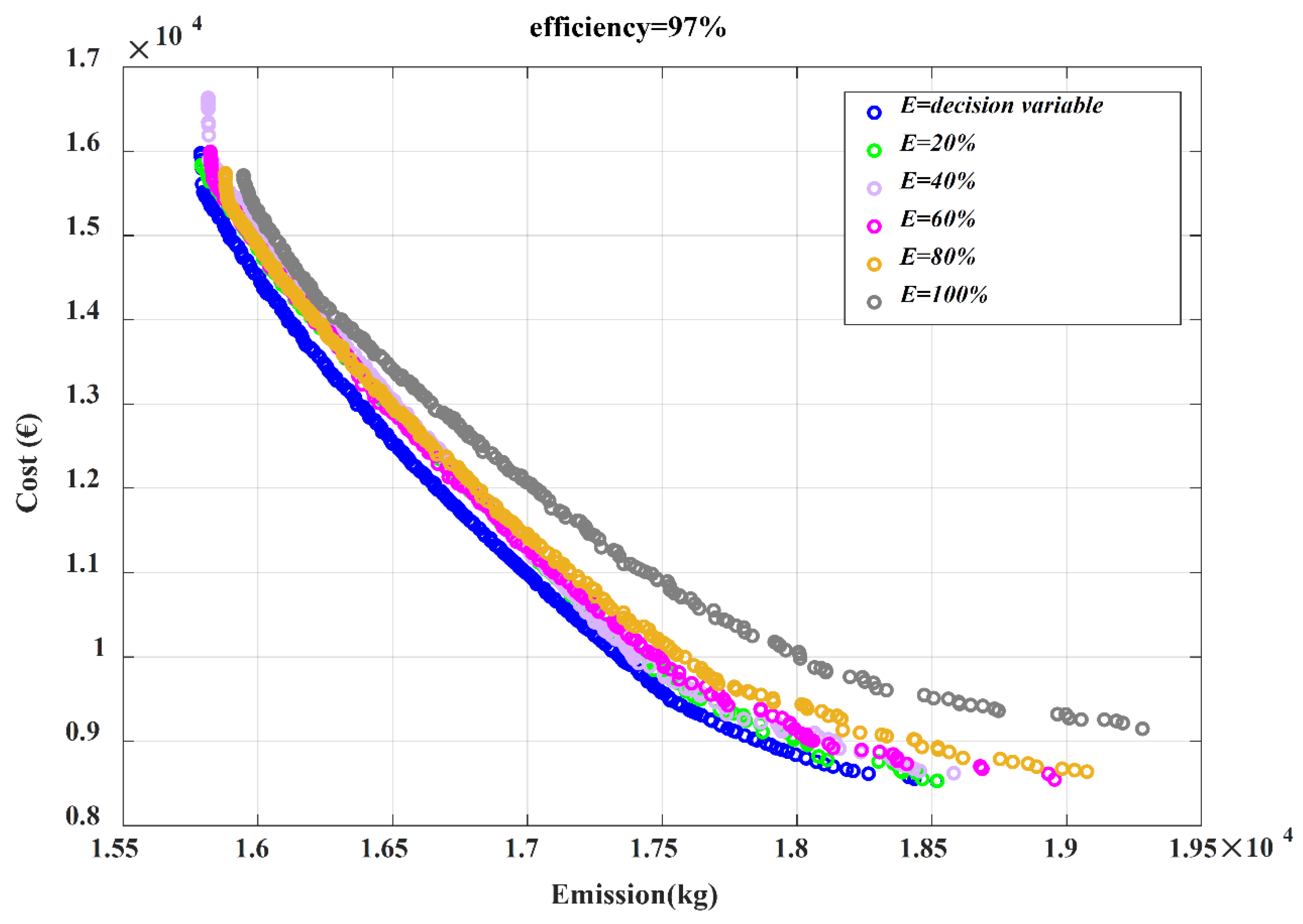
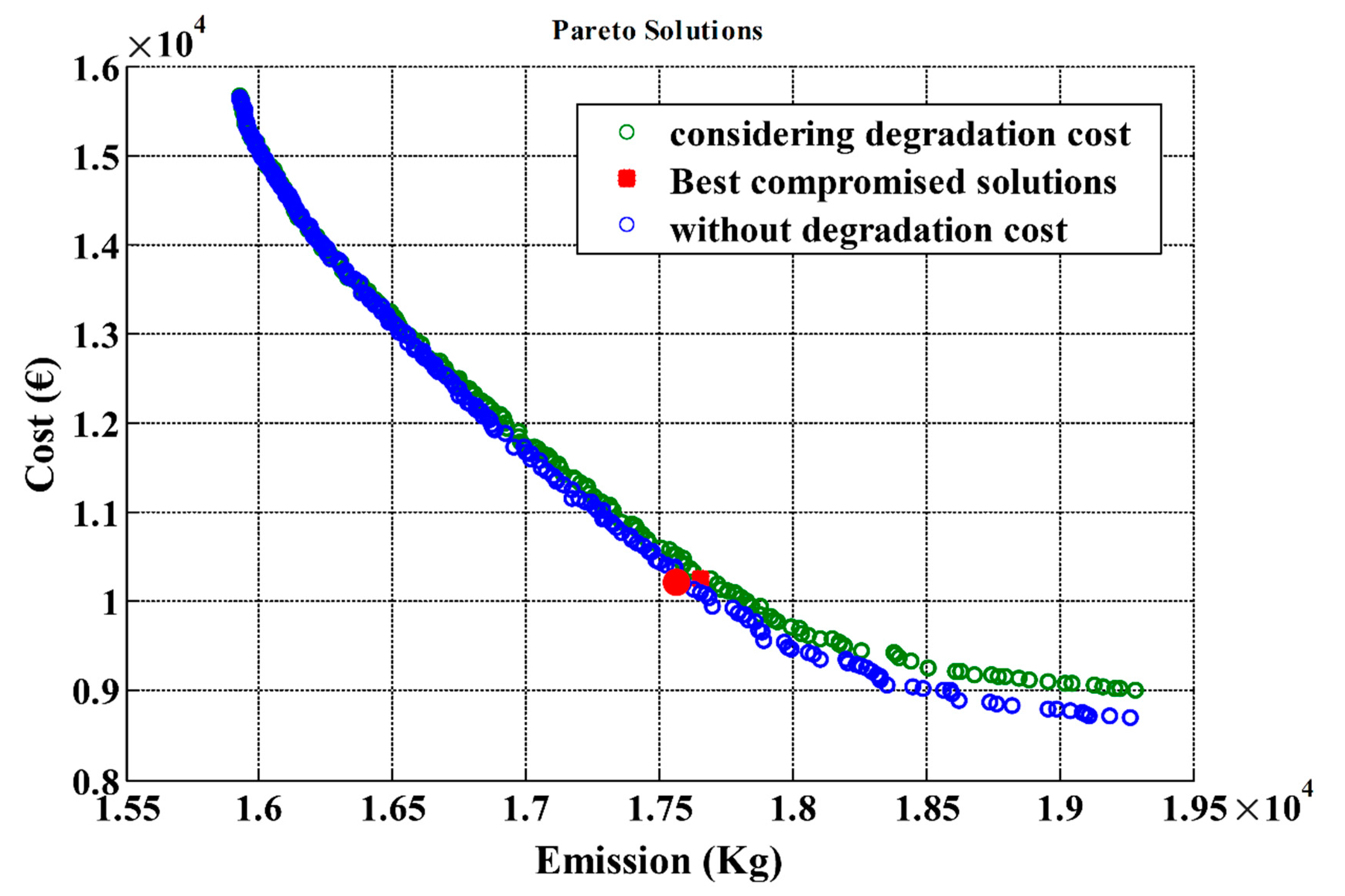
  • The power constraints of the storage device (i.e., Li-ion battery in this study) as well as the degradation cost are considered in the MG’s MOOM problem. In order to consider different battery characteristics, including the battery efficiency, the battery’s initial charge, SOC, and different scenarios of the battery’s degradation cost are studied in the probabilistic MG’s MOOM problem.
  • Modifications are added to the JAYA algorithm that make it more efficient in dealing with multi-objective problems. The efficiency of the suggested algorithm is examined by comparing its performance with some other well-known algorithms.
  • The total cost of day-ahead market transactions and fuel costs, along with the emission of MG, are minimized through the introduced optimal scheduling approach. The suggested RUT-EMOJAYA reduces the MG’s dependency on the main grid and the electricity market, while maximizing the utilization of RESs in the studied region.
  • The uncertainties related to the forecasted values of the load demand and market price, and the available outputs of RESs, as well as their correlations, are considered and dealt with efficiently using the suggested RUT-EMOJAYA.
The remainder of this paper is organized as follows: the economic model of the storage device is described in Section 2. In Section 3, the problem is formulated and the objective functions along with the constraints are presented. The RUT method is discussed in Section 4. Section 5 is devoted to the presentation of the applied algorithm. In Section 6, the applied methodology for solving MOOM in an ordinary MG is explained. Results are investigated in Section 7. Finally, the conclusions are highlighted in Section 8.

2. Economic Model of Battery Storage Devices

An economic model of storage devices is presented in this section. As dispatchable units, storage devices can be charged in low demand hours, while they discharge in peak load hours when there is a power shortage in the system [31]. In this paper, the degradation cost of the storage device is added to the operational cost of the system in order to improve the cost objective function. During the discharge hours, the degradation cost is a function of a number of factors, including the battery DoD at start and end of the discharging process, the investment cost and the usable energy of the battery, as well as battery-specific parameters [32]. Different factors can affect the N c y c l e of a battery, including, DoD, discharge rate, ambient temperature, charging regime, etc. N c y c l e is defined as the number of complete charge–discharge cycles that the battery can undergo before its nominal capacity falls below 80% of its initial rated capacity [31].
DoD is an absolute discharge relative to the rated battery capacity that is a function of the battery’s state of charge (SOC). SOC ( S O C ( t ) = Q ( t ) Q n ) is defined as the ratio of the battery’s current capacity, Q(t) (kWh), to the battery’s nominal capacity, Q n (kWh). Q n is representative of the maximum amount of charge that can be stored in the battery and is given by the manufacturer [33]. In this paper, the DoD of the battery is considered as follows [32]:
D o D t = E B a t t , max E t E B a t t , max
where E B a t t , max is the maximum energy stored in the battery and Et is the energy stored in the battery at a specific hour of the day. The cycle life of the battery is as follows:
N c y c l e = a . D o D b
where a and b are battery-specific parameters considered equal to 1331 and −1.825, respectively, for Li-ion batteries [32]. Consequently, the battery degradation cost C o s t D e g t is formulated as:
C o s t D e g t = C B a t t . D o D . E B a t t N c y c l e
where C B a t t is the investment cost of the battery, and E B a t t is the usable energy of the battery [32].

3. Problem Formulation

3.1. Objective Functions

The first objective is to minimize the total operation cost as presented in the following [33]:
F 1 ( X ) = t = 1 T C o s t t = t = 1 T { i = 1 N D G [ u i t . ( P D G i t ) . B D G i t + S U C D G i . u i t . ( 1 u i t 1 ) + S D C D G i . u i t 1 . ( 1 u i t ) ] + r = 1 N R E S [ P R E S r t . B R E S r t ] + s = 1 N B a t t [ P B a t t s t . B B a t t s t + C o s t D e g t ] + P G r i d t . B G r i d t }
X = [ U D G , P D G , P B a t t , P G r i d ] 1 × n
n = [ ( ( 2 × N D G ) + N B a t t ) + 1 ] × T
U D G = [ u 1 , u 2 , , u N D G ] = { u i } 1 × N D G { 0 , 1 }
u i = [ u i 1 , u i 2 , , u i t , , u i T ] ; i = 1 , 2 , , N D G
P D G = [ P D G 1 , P D G 2 , , P D G N D G ]
P D G i = [ P D G i 1 , P D G i 2 , , P D G i t , , P D G i T ] ; i = 1 , 2 , , N D G
P B a t t = [ P B a t t 1 , P B a t t 2 , , P B a t t N B a t t ]
P B a t t , s = [ P B a t t , s 1 , P B a t t , s 2 , , P B a t t , s t , , P B a t t , s T ] ; s = 1 , 2 , , N B a t t
P R E S = [ P R E S 1 , P R E S 2 , , P R E S N R E S ]
P R E S r = [ P R E S r 1 , P R E S r 2 , , P R E S r t , , P R E S r T ] ; r = 1 , 2 , , N R E S
P G r i d = [ P G r i d 1 , P G r i d 2 , , P G r i d t , , P G r i d T ]
where DG demonstrates the dispatchable units including fuel cell (FC) and micro-turbine (MT), while Grid and Batt present the utility grid and the battery, respectively. The WT and photovoltaic (PV) are shown with RES as non-dispatchable units. Note that the utility has to buy all of the electrical power produced by RES units; consequently, the RESs’ output powers ( P R E S , r t ) are not included in the design variables’ vector; u i t is applied to imply the on/off states of the ith dispatchable DG during each hour of the day.
The minimization of environmental pollutants is considered as the second objective as follows [33]:
F 2 ( X ) = t = 1 T E m i s s i o n t = t = 1 T { i = 1 N D G [ u i t . ( P D G i t ) . E G i t ] + s = 1 N B a t t [ P B a t t s t . E B a t t s t ] + P G r i d t . E G r i d t }
where the extent of produced pollutants in one hour of the MG’s operation is shown by Emission t [5]:
E D G i t = C O 2 D G i t + S O 2 D G i t + N O x D G i t
E B a t t s t = C O 2 B a t t , s t + S O 2 B a t t , s t + N O x B a t t , s t
E G r i d t = C O 2 G r i d t + S O 2 G r i d t + N O x G r i d t
In the equations above, C O 2 D G i t , S O 2 D G i t and N O x D G i t are the levels of CO2, SO2 and NOx emissions from the ith DG source; C O 2 B a t t , s t , S O 2 B a t t , s t and N O x G r i d t are the amounts of CO2, SO2 and NOx emission from the sth battery unit and C O 2 G r i d t , S O 2 G r i d t and N O x G r i d t are the amounts of CO2, SO2 and NOx emission from the utility at hour t, respectively [5].

3.2. Constraints

3.2.1. Power Balance Constraint

The balance of electricity demand and power supply is one of the most important requirements in MG energy management [33]; hence:
i = 1 N D G [ u i t . P D G i t ] + r = 1 N R E S [ P R E S r t ] + s = 1 N B a t t [ P B a t t s t ] + P G r i d t = P L D t
where P L D t is the total MG load at hour t.

3.2.2. Battery Limits

The constraints of the battery SOC limits during each time interval are considered as follows [34]:
W B a t t s , min W B a t t t s W B a t t s , max
where W B a t t t s is the SOC of the sth battery at the end of one-hour interval, which is associated with the time t as follows:
E B a t t t = E B a t t t 1 + η c P c h . Δ t 1 η d P d i s c h . Δ t
P c h t P c h , max
P d i s c h t P d i s c h , max
where E B a t t t and E B a t t t 1 are the energies stored inside the battery at hours t and t − 1, respectively. The lower and upper limits of the stored energy inside the sth battery are E B a t t s , min and E B a t t s , max .
Additionally, E B a t t t should not violate the following limits:
0.1 E B a t t , max E B a t t t E B a t t , max

3.2.3. Real Power Constraints

Power generations of each dispatchable DG are limited as follows:
u i t . P D G i , min t P D G i t u i t . P D G i , max t
The power exchange with the utility grid is constrained as follows:
P G r i d , min t P G r i d t P G r i d , max t
The following shows the constraints of the battery rates of charge and discharge during each hour:
P B a t t s , min t P B a t t s t P B a t t s , max t

4. Reduced Unscented Transformation (RUT)

Wind power generation, solar irradiation, load demand and market price are the most important, uncertain parameters to be considered for solving the problem of MGs’ optimal operation. In this paper, the RUT method is used to model uncertainties based on [29]. The uncertain variables follow a normal distribution function with mean values equal to those expressed in [29] and standard deviations equal to 10% of their mean values. The main steps followed by the RUT method are summarized in the following [29].
Step 1: Choose 0 ≤ W0 ≤ 1:
Step 2: Choose weight sequence according to the following criterion:
W k = ( 1 W 0 ) ( m + 1 ) ,   k = 1 , , m + 1
Step 3: Initialize vector sequence:
Step 4: Expand vector sequence ( ξ k j ) for j = 2,…, m according to the following:
[ ξ 0 j 1 0 ] k = 0 , [ ξ k j 1 1 j ( j + 1 ) W 1 ] k = 1 , , j , [ 0 j 1 j j ( j + 1 ) W 1 ] k = j + 1
If a random variable vector Z has a mean μ z and a covariance matrix P z z , the kth sigma point is:
Z k j = μ z + P z z ξ k j ξ 0 1 = [ 0 ] , ξ 1 1 = [ 1 2 W 1 ] , ξ 2 1 = [ 1 2 W 1 ]
where P z z is a matrix square root of P z z . For a positive definite matrix P, the matrix square root means that a matrix A = P exists such that P = A A T , which should be calculated using numerically efficient and stable methods such as Cholesky decomposition [35]. If there is no correlation between uncertain variables, the elements of P z z ’s main diameter will be the square of uncertain variables’ standard deviations ( σ ). However, in correlated conditions, depending on which uncertain variables are correlated, the corresponding elements of the rows and columns of P z z may have negative or positive values. Accordingly, the P z z matrix can be obtained as follows:
P z z = [ p z z ( α , β ) ] m × m α , β = 1 , 2 , , m p z z ( α , α ) = σ i 2 α = β p z z ( α , β ) = γ α , β . σ α . σ β α β
where γα,β is the correlation coefficient between the αth and βth elements of the covariance matrix Pzz.
Step 5: Input m + 2 sigma points to the function to find the output samples:
Y k = f ( Z k )
Step 6: Calculate the mean μ y and covariance matrix P y y of the output Y as follows:
Ε ( y ) = μ y = k = 0 m + 1 W k Y k
P y y = k = 0 m + 1 W k ( Y k μ y ) ( Y k μ y ) T

5. Enhanced Multi-Objective JAYA Algorithm

5.1. A Brief Overview of the Original JAYA

The JAYA algorithm, which was proposed by “R. Venkata Rao” [28], is enhanced and applied in this article. The inspiration of the original JAYA algorithm is derived from the Sanskrit word “JAYA” the meaning of which is “victory”. In the JAYA algorithm, each individual moves toward the best solution while trying to move far away from the worst in order to achieve the best solution. As the methodology is demonstrated in the following, due to the simplicity and rapidity of the algorithm, and since there is no need to have any information regarding control parameters, JAYA becomes more advantageous compared to other meta-heuristic algorithms [28,29].
The goal is to minimize F ( X ) as the objective function. Assume that the best solution, ‘ X b e s t ’, and the worst solution, ‘ X w o r s t ’, obtain the best and the worst values of F ( X ) in the entire candidate solutions, respectively. Let X i , i t e r n e w be the ith candidate during the iterth iteration. Then, to modify the decision variables, individuals could be changed according to the following [28]:
X i , i t e r n e w = X i , i t e r + r 1 , i , i t e r ( X b e s t X i , i t e r ) r 2 , i , i t e r ( X w o r s t X i , i t e r )
where r1 and r2 are random variables in [0, 1], X b e s t is the best solution in each iteration, while X w o r s t is the worst solution in the population; X i , i t e r n e w will be accepted if its objective function value is better than that of X i , i t e r .

5.2. Multi-Objective JAYA (MOJAYA)

Since, in this paper, a multi objective problem is implemented, new definitions should be considered for ‘ X b e s t ’ and ‘ X w o r s t ’. For this purpose, the initial population should be organized according to the following [35]:
B C S = M i n ( ω 1 ( f 1 n d f 1 m i n f 1 m a x f 1 m i n ) + ω 2 ( f 2 n d f 2 m i n f 2 m a x f 2 m i n ) ) n d = 1 , 2 , , N n o n _ d o m
where f 1 and f2 are the cost and emission of the objective functions, respectively. The initial guess for ω1 and ω2 is equal to 0.5 [36]. The worst solution is the most dominant solution in each iteration and is then selected as ‘ X w o r s t ’. In order to select the best solution, in each iteration, after choosing the non-dominated solutions and controlling the size of the repository according to Algorithm 1, the best solution is selected from the repository as ‘ X b e s t ’ based on (33) and is used in the subsequent iterations.
Algorithm 1. Pseudo code for controlling the size of repository.
1: κ = [ 0 ]
2: for i = 1 t o N n o n d o m 1
3:       for  j = i + 1 t o N n o n d o m
4:            distance = m = 1 M ( f i m f j m ) 2
5:            if distance < Epsilon
6:               κ j = κ j + 1
7:           end
8:       end
9:   end
10: sort non-dominated solutions ascending according to κ j
11: save the first N L elements of the non-dominated solutions in the repository
where κ is a column matrix, the dimension and the elements of which are the number of non-dominated solutions, and the counters related to each non-dominated solution, respectively. N n o n d o m is the number of non-dominated solutions, f i and f j are the objective functions, and M is the number of objective functions. N L is a predefined value, and when the size of the repository exceeds N L , the repository size will be controlled by comparing the distances of the stored, non-dominated solutions [37,38].

5.3. Enhanced MOJAYA (EMOJAYA)

When the dimensions of the problem increase, the original JAYA may not find the global optimum solution easily. Consequently, in order to achieve a real and well-scattered Pareto optimal front, and for improving the performance, convergence ability and the accuracy of the algorithm, some modifications are necessary. In the suggested EMOJAYA algorithm, the main superiority of the original JAYA, which is independency to algorithmic parameters, is also preserved. The modification process of the algorithm is as follows:
Step 1: Set i = 1
Step 2: Select the ith individual from the initial population.
Step 3: Choose five constants k 1 k 2 k 3 k 4 k 5 , unequal to i, randomly from the initial population, and select three constants k 1 k 2 k 3 from the repository.
Step 4: Calculate four new individuals as follows:
X i , n e w 1 = X k 1 + r a n d × ( X k 2 X k 3 )
X i , n e w 2 = X n e w 1 + r a n d × ( X b e s t X w o r s t )
X i , n e w 3 = X k 4 + r a n d × ( X b e s t X k 5 )
X i , n e w 4 = X k 1 + r a n d × ( X k 2 X k 3 )
Step 5: Calculate objective functions for the new individuals.
Step 6: Determine and save non-dominated solutions.
Step 7: Update X i from the new non-dominated solutions of Step 6 using (32).
Step 8: If all individuals are updated, stop; otherwise, set i = i + 1 and return to Step 2.

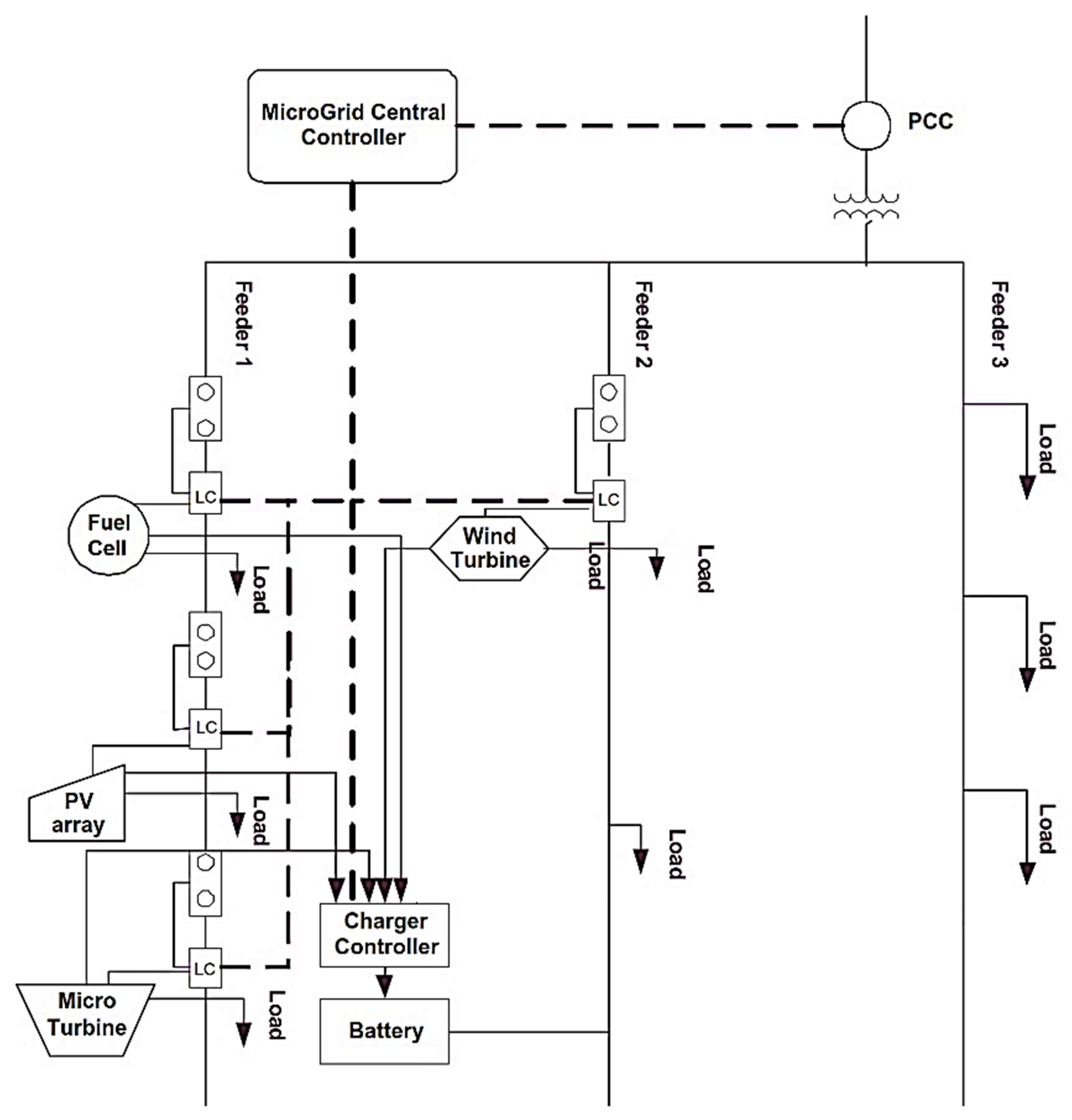
6. Application of the Suggested EMOJAYA Algorithm

In order to apply the proposed EMOJAYA algorithm on the considered MOOM problem, the following steps should be taken:
Step 1: Initialize the population size, number of design variables and termination criterion. Problem information including MG properties, as well as bids and power information of DGs, storages and utility and emission coefficients shall be specified. The initial charge of the battery is also defined in this step.
Step 2: Hourly WT and PV power forecasts, demand and electricity price are determined through RUT.
Step 3: Since a mixed-integer problem is considered in this study, two types of variables, i.e., binary and continuous, are assumed. For states of generators as binary variables, ui s according to (5) are generated as follows:
u i t = r o u n d ( r a n d 4 ( . ) × ( u i , max t u i , min t ) + u i , min t )
However, in order to consider the states of dispatchable units, U i t should satisfy the following condition for all hours:
i = 1 N D G [ u i t . P D G i , min t ] + r = 1 N R E S [ P R E S r , min t ] + s = 1 N B a t t [ P B a t t s , min t ] + P G r i d min t P L o a d t i = 1 N D G [ u i t . P D G i , max t ] + r = 1 N R E S [ P R E S r , max t ] + s = 1 N B a t t [ P B a t t s , max t ] + P G r i d max t
If the equation above is satisfied, a random population for continuous variables based on the achieved ui s and according to (5) must be generated as follows:
P D G i t = r a n d 5 ( . ) × ( P D G i , max t P D G i , min t ) + P D G i , min t
P B a t t s t = r a n d 6 ( . ) × ( P B a t t s , max t P B a t t s , min t ) + P B a t t s , min t
P G r i d t = r a n d 7 ( . ) × ( P G r i d , max t P G r i d , min t ) + P G r i d , min t
while the power constraints in (12)–(14) should be satisfied.
Step 4: Since in the considered problem, some limitations, such as battery constraints, depend on previous and future hours, constraints change in different hours of the day as follows:
For discharging mode:
E d i s c h , B a t t t + 1 = max { ( E B a t t t Δ t P B a t t t η d ) , E B a t t , min } , t = 1 , , T
For charging mode:
E c h , B a t t t + 1 = min { ( E B a t t t Δ t P B a t t t , η c ) , E B a t t , max } , t = 1 , , T
where for both discharging and charging modes:
P c h , max P B a t t t P d i s c h , max , t = 1 , , T
P d i s c h , max t = min { ( P B a t t , max , ( E B a t t t E B a t t , min ) η d Δ t ) } , t = 1 , , T
P c h , max t = max { ( P B a t t , min , ( E B a t t t E B a t t , max ) ( η c Δ t ) ) } , t = 1 , , T
The limitation of the released energy in the discharging mode and the stored energy in charging mode are mentioned in (27) and (28), respectively, while (30) and (31) demonstrate the power discharged by the battery in the discharge mode and the power charged by the grid in the charging mode. Using (30) and (31), the maximum and minimum rates of charging and discharging modes can be calculated [16].
Step 5: Calculate the objective functions for the population.
Step 6: Determine the non-dominated solutions in the population and store them in the repository.
Step 7: Choose ‘Xbest’ and ‘Xworst’ as described in Section 5.1.
Step 8: Update the initial population as Section 5.
Step 9: Determine the non-dominated solutions in the new population.
Step 10: Update the repository based on new and old non-dominated solutions.
Step 11: If the number of non-dominated solutions is more than a predefined value, NL, control the size of the repository according to Algorithm 1.
Step12: Control the termination criterion (iteration = iterationmax). If it is satisfied, terminate the algorithm; otherwise, set iteration = iteration + 1 and return to Step 7.
Step 13: Report the BCS that is achieved using the technique proposed in Section 5.1.

7. Simulation Results

In order to justify the efficient performance and competitiveness of the proposed EMOJAYA algorithm, two subsections are investigated in this section. First, the performance of the suggested EMOJAYA is compared with the original JAYA and PSO algorithms by applying these algorithms (40 independent runs of each algorithm are performed, and the results are reported) to three test functions of [39]. In the second sub-section, three different scenarios are considered to inspect the effectiveness of the EMOJAYA algorithm in solving MG energy management problems in the presence of storage devices.

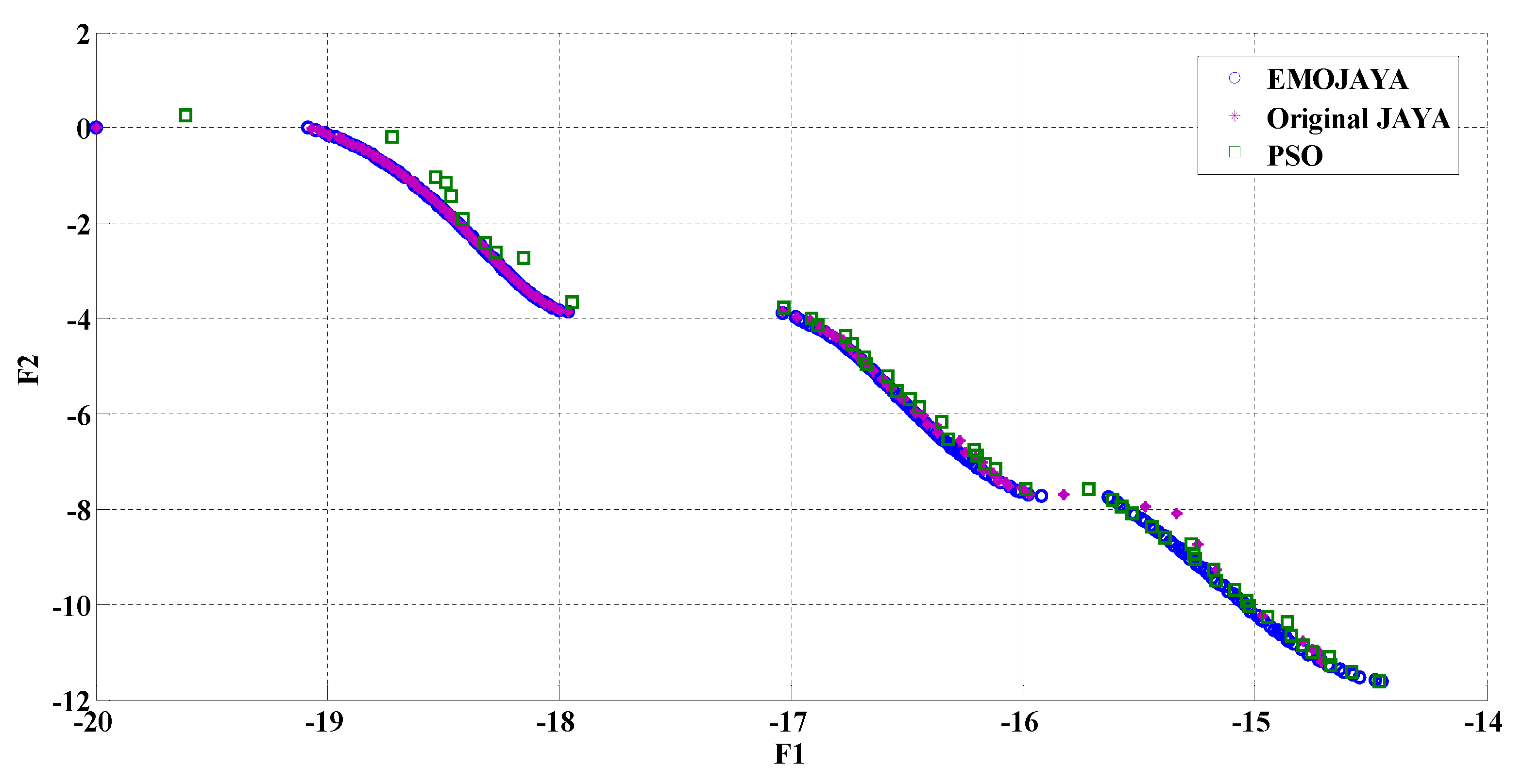
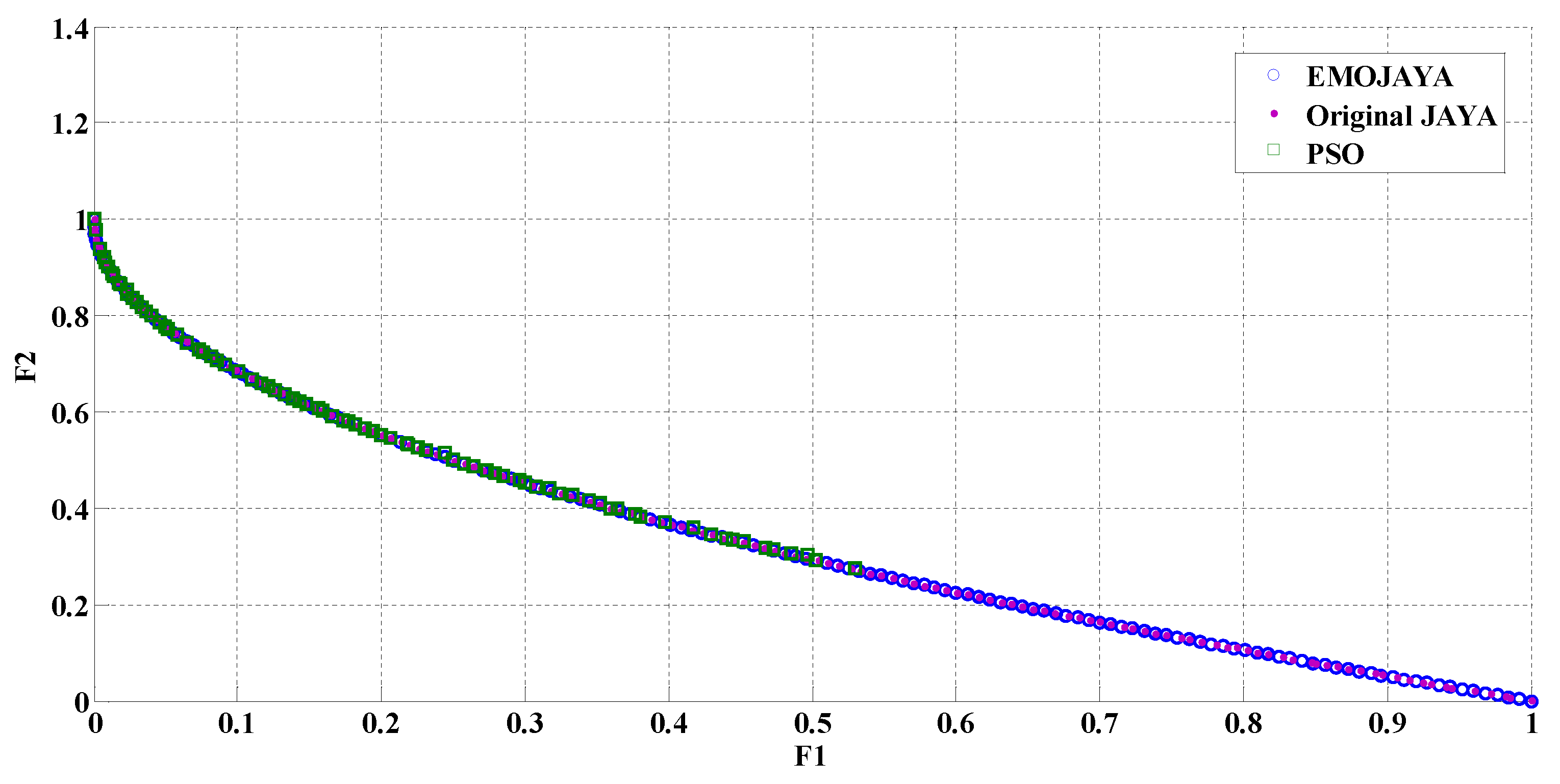
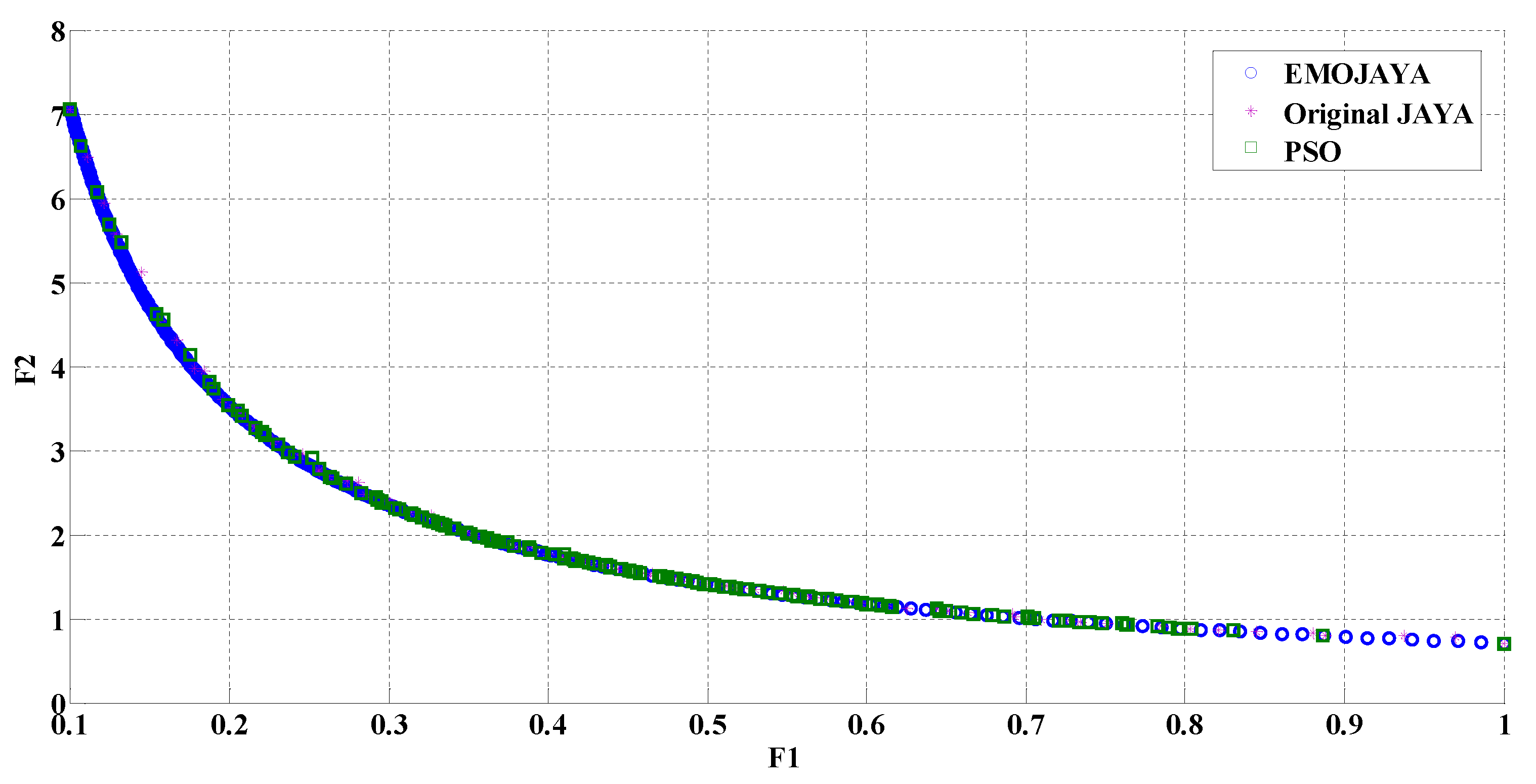
7.1. A Comparison between the Performance of Proposed EMOJAYA with Original JAYA and PSO Algorithms on Different Test Functions

In this section, three different test functions of [39] are considered and the proposed EMOJAYA algorithm is applied to solve the problems.
-Test Function 1: The first test objective functions of [39] are as follows:
M i n i m i z e f 1 ( x ) = i = 1 n 1 ( 10 exp ( 0.2 x i 2 + x i + 1 2 ) ) M i n i m i z e f 2 ( x ) = i = 1 n ( | x i | 0.8 + 5 sin ( x i ) 3 )
where 5 x 1 , x 2 , x 3 5
The Pareto front of the suggested EMOJAYA and those of the original JAYA and PSO are compared in Figure 2, and the prior performance of EMOJAYA in solving the first chosen test function is observed.
-Test Function 2: The second proposed benchmark in [39] is as follows:
M i n i m i z e f 1 ( x 1 , x 2 ) = x 1 M i n i m i z e f 2 ( x 1 , x 2 ) = g ( x 1 , x 2 ) . h ( x 1 , x 2 )
where:
g ( x 1 , x 2 ) = 11 + x 2 2 10 . cos ( 2 π x 2 ) h ( x 1 , x 2 ) = { 1 f 1 ( x 1 , x 2 ) g ( x 1 , x 2 ) , i f   f 1 ( x 1 , x 2 ) = x 1 0 , o t h e r w i s e
and 0 x 1 1 , 30 x 2 30
Figure 3 shows the performance and the resulting Pareto front of EMOJAYA, original JAYA and PSO algorithms for solving the second test case study. It is observed that the suggested EMOJAYA has a better performance compared to the two other algorithms.
-Test Function 3: The third test function is [39]:
M i n i m i z e f 1 ( x 1 , x 2 ) = x 1 M i n i m i z e f 2 ( x 1 , x 2 ) = g ( x 2 ) x 1
g ( x 2 ) = 2 exp { ( x 2 0.2 0.004 ) 2 } 0.8 exp { ( x 2 0.6 0.4 ) 2 }
and 0.1 x 1 1 , 0.1 x 2 1
In Figure 4, the Pareto front of the proposed EMOJAYA and the results of the original JAYA and PSO are demonstrated. It can be concluded that EMOJAYA has a better performance compared to PSO and JAYA algorithms.
From Figure 2, Figure 3 and Figure 4, and by comparing the Pareto optimal fronts of the investigated algorithms, it is clear that the proposed EMOJAYA has an efficient performance in solving multi-objective problems.

7.2. Solving the MG Energy Managemnet Problem

In this section, three different scenarios are investigated to verify the effectiveness of the proposed RUT-EMOJAYA algorithm in solving the probabilistic MG energy management problem in the presence of storage devices. The MG of Figure 1 is considered as the test system. A 24-hour scheduling scheme is assumed for the analysis of the simulated system. For all DGs, the unity power factor is considered; thus, they only produce active power. The MGCC is responsible for controlling the power exchange between the MG and the utility, which is allowed at any hour in a day in order to more profitably exploit the market. The hourly active power of PV and WT, the forecasted load demand, and the utility power production bid are shown in Figure 5 and Figure 6. It is assumed that all loads are electrical [40].
In Table 1, the entire bid data for all DGs and utility grid, as well as the amount of emission of DGs, are available [41]. Since PV and WT units do not consume any fuel when they produce electric power, the utility grid has to buy all electric power produced by these units [5]. Since the two considered objective functions (cost and emission) are conflicting, a Pareto-optimal set is achieved for each considered case.
The proposed method was implemented in MATLAB. The number of both populations and maximum iterations is considered to be 100.
The on\off states of dispatchable DGs (i.e., FC and MT) are taken into account in the considered MG’s energy management problem. Therefore, in the algorithm process, if the solutions for dispatchable units are lower than their minimum limit powers, then the power will be set to zero.
Three scenarios are studied in this section to investigate the effect of storage devices on solving the MOOM problem. In the two first scenarios, it is assumed that the battery has a degradation cost, as in (3), while in the third scenario, a comparison between the situations with and without considering the battery degradation cost is carried out.
Scenario I: In this case, the battery efficiencies are considered to be 93%, 95% and 97%, taking the influence of the Li-ion battery efficiency into account. Additionally, the impact of different initial and final charges is contemplated in the three aforementioned efficiencies. In each case, the battery’s initial and final charges (initial charge = final charge = E) differ from E B a t t , max to 0.2 E B a t t , max so that this variation effect can be investigated. Accordingly, the comparison of cost and emission objective functions in the BCS point for different efficiencies, including 93%, 95% and 97%, are shown in Figure 7, Figure 8 and Figure 9. Moreover, the Pareto optimal front for different efficiencies, along with their BCS points are illustrated in Figure 10. It should be mentioned that, in Figure 10, results are compared for the case that E is equal to E B a t t , max .
Scenario II: In the second scenario, in order to obtain the best value of the battery initial and final charges (initial charge = final charge = E), they are considered as decision variables. Figure 11, Figure 12 and Figure 13 show comparisons of the Pareto optimal fronts for different E values in different efficiencies (i.e., 93%, 95% and 97%). It can be observed from Figure 11, Figure 12 and Figure 13 that when E is considered as a decision variable, a better Pareto optimal front is achieved in all efficiencies and, consequently, the obtained BCS will be more convenient.
Scenario III: In the third scenario, the battery degradation cost is neglected and results are compared with the situation in which the battery degradation cost is taken into account as Equation (3). In this case, the battery efficiency is considered equal to 95%. The comparison of Pareto optimal fronts with and without considering degradation cost is given in Figure 14. According to this figure, as already expected, the Pareto optimal front reveals a drop in cost objective function when the degradation cost is ignored.
The advantage and perfection of an optimization algorithm for solving multi-objective problems is decided based on its effective and fast convergence, resulting in a smooth and accurate Pareto front. According to the simulation results, it is confirmed that the presented EMOJAYA algorithm successfully satisfies these criteria.

8. Conclusions

The probabilistic economic/emission optimal operation of a typical MG was dealt with in this paper using the new RUT-EMOJAYA algorithm. In order to investigate the role of storage devices, as well as the effective performance of the suggested algorithm, three different scenarios were studied. In the first case, different efficiencies for the storage device were considered, while the battery’s initial and final charges were not included in the decision variables. Simulation results showed that, by increasing the battery efficiency from 93% to 97%, the daily operational cost of the MG system was reduced from EUR 9200 to EUR 8900. In the second case, the battery’s initial and final charges were considered as decision variables, and it was observed that the Pareto optimal front in this case was better distributed than in the previous case. In the third case, the degradation cost of the storage device was ignored in order to compare the results with those of other two cases where this cost was taken into account. It was seen that the Pareto optimal front, without considering the degradation cost, demonstrated a decrease (USD 270) in the minimum achievable daily operation cost of the MG system, which is expected to be true. It was concluded that the proposed method for dealing with mixed-integer optimization problems in the presence of uncertainties is accurate. It should be pointed out that as the RUT-EMOJAYA algorithm is comparably simple and not dependent on control parameters, its application is recommended for clarifying other problems. Future studies can include the following:
i.
Investigating elements of the future smart grids, including demand response and the influence of electric vehicles on the considered MG’s energy management problem.
ii.
Inspecting reliability as an objective function in the MG’s optimal operation management.
iii.
Comparing different energy storage devices, as well as a variety of battery technologies to decide on the most optimal economic design of the system.

Author Contributions

Conceptualization, M.J. and H.P.A.; methodology, M.J., H.P.A. and T.K.; software, M.J. and H.P.A.; validation, M.J., H.P.A. and T.K.; formal analysis, M.J.; investigation, M.J; writing—original draft preparation, M.J.; writing—review and editing, T.K., D.S., S.S. and J.M.G.; supervision, T.K., D.S., S.S. and J.M.G. All authors have read and agreed to the published version of the manuscript.

Funding

This research was funded by the European Union’s Horizon 2020 research and innovation programme under the Marie Sklodowska-Curie grant agreement No 812991. J. M. Guerrero was supported by VILLUM FONDEN under the VILLUM Investigator Grant (no. 25920): Center for Research on Microgrids (CROM); www.crom.et.aau.dk, accessed date: 15 October 2021.

Institutional Review Board Statement

Not applicable.

Informed Consent Statement

Not applicable.

Data Availability Statement

Not applicable.

Conflicts of Interest

The authors declare no conflict of interest.

Nomenclature

RESrenewable energy source
MGmicrogrid
DERdistributed energy source
PSOparticle swarm optimization
ODEDoptimal dynamic economic dispatch
WTwind turbines
DGdistributed generator
MOOMmulti-objective optimal operation management
PCCpoint of common coupling
LClocal controller
MGCCmicro grid central controller
EMOJAYAenhanced multi-objective JAYA
RUTreduced unscented transformation
SOCstate of charge
DoDdepth of discharge
FCfuel cell
MTmicro-turbine
PVphotovoltaic
BCSbest-compromised solution
X vector of decision variables
Nnumber of decision variables
Ttotal number of hours
N c y c l e battery cycle life
Qnbattery nominal capacity (kWh)
Q(t)battery current capacity (kWh)
C o s t D e g t battery degradation cost (EUR) at hour t
CBattbattery investment cost (EUR/kWh)
NDGtotal number of dispatchable generations
NBatttotal number of batteries
NREStotal number of RESs
Ndtotal number of load levels
CosttMG’s operation cost in hour t (EUR)
P R E S , r t real output powers (kWh) of rth RES at hour t
P D G , i t real output powers (kWh) of ith DG at hour t
P B a t t , s t real output powers of sth storage at hour t
P G r i d t active power bought (sold) from (to) the utility at hour t
B R E S , r t bids of RESs at hour t (EUR/kWh)
B D G i t bids of dispatchable DGs at hour t (EUR/kWh)
B B a t t , s t bids of battery at hour t (EUR/kWh)
B G r i d t bids of the utility grid at hour t (EUR/kWh)
S U C D G i start-up cost for ith dispatchable DG
S D C D G i shut down cost for ith dispatchable DG
( P D G i t . B D G i t ) operational cost of dispatchable DGs
( P R E S r t . B R E S r t ) operational cost of RESs
( P B a t t s t . B B a t t s t ) operational cost of battery
( P G r i d t . B G r i d t ) cost of power exchange between the MG and the utility grid (EUR)
PLDamount of dth load level
E D G i t amount of pollutants emission for each generator at hour t (kg/MWh)
E B a t t s t amount of pollutants emission for storage device at hour t (kg/MWh)
E G r i d t amount of pollutants emission for the utility grid at hour t (kg/MWh)
W B a t t t amounts of energy stored inside the battery at hour t
Pch (Pdisch) permitted rate of charge (discharge) of the battery
ηc (ηd)efficiency of the battery during charge (discharge) process
W B a t t s , min lower limit of amounts of energy storage inside the battery
W B a t t s , max upper limit of amounts of energy storage inside the battery
P c h , max ( P d i s c h , max ) maximum rate of battery charge (discharge) during each time interval ∆t
P D G , min t minimum active power of the ith DG
P D G , max t maximum active power of the ith DG
P B a t t , min t minimum active power of the bth storage
P B a t t , max t maximum active power of the bth storage
P G r i d , min t minimum active power of the utility at hour t.
P G r i d , max t maximum active power of the utility at hour t.
P L D load demand

References

  1. Ali, S.; Zheng, Z.; Aillerie, M.; Sawicki, J.P.; Péra, M.C.; Hissel, D. A Review of DC Microgrid Energy Management Systems Dedicated to Residential Applications. Energies 2021, 14, 4308. [Google Scholar] [CrossRef]
  2. Javidsharifi, M.; Pourroshanfekr, H.; Kerekes, T.; Sera, D.; Spataru, S.; Guerrero, J.M. Optimum Sizing of Photovoltaic and Energy Storage Systems for Powering Green Base Stations in Cellular Networks. Energies 2021, 14, 1895. [Google Scholar] [CrossRef]
  3. Linden, D.; Reddy, T. Handbook of Batteries, 3rd ed.; McGraw-Hill Professional: New York, NY, USA, 2001. [Google Scholar]
  4. González, A.; Goikolea, E.; Barrena, J.A.; Mysyk, R. Review on Supercapacitors: Technologies and Materials. Renew. Sustain. Energy Rev. 2016, 58, 1189–1206. [Google Scholar] [CrossRef]
  5. Javidsharifi, M.; Niknam, T.; Aghaei, J.; Mokryani, G. Multi-objective short-term scheduling of a renewable-based microgrid in the presence of tidal resources and storage devices. Appl. Energy 2018, 216, 367–381. [Google Scholar] [CrossRef] [Green Version]
  6. Rezvani, A.; Gandomkar, M.; Izadbakhsh, M.; Ahmadi, A. Environmental/economic scheduling of a micro-grid with renewable energy resources. J. Clean. Prod. 2015, 87, 216–226. [Google Scholar] [CrossRef]
  7. Modiri-Delshad, M.; Kaboli, S.H.A.; Taslimi-Renani, E.; Abd Rahim, N. Backtracking search algorithm for solving economic dispatch problems with valve-point effects and multiple fuel options. Energy 2016, 116, 637–649. [Google Scholar] [CrossRef]
  8. Hemmati, R.; Saboori, H.; Jirdehi, M.A. Stochastic planning and scheduling of energy storage systems for congestion management in electric power systems including renewable energy resources. Energy 2017, 133, 380–387. [Google Scholar] [CrossRef]
  9. Soares, J.; Silva, M.; Sousa, T.; Vale, Z.; Morais, H. Distributed energy resource short-term scheduling using Signaled Particle Swarm Optimization. Energy 2012, 42, 466–476. [Google Scholar] [CrossRef] [Green Version]
  10. Zhang, J.; Wu, Y.; Guo, Y.; Wang, B.; Wang, H.; Liu, H. A hybrid harmony search algorithm with differential evolution for day-ahead scheduling problem of a microgrid with consideration of power flow constraints. Appl. Energy 2016, 183, 791–804. [Google Scholar] [CrossRef]
  11. Gupta, R.A.; Gupta, N.K. A robust optimization based approach for microgrid operation in deregulated environment. Energy Convers. Manag. 2015, 93, 121–131. [Google Scholar] [CrossRef]
  12. Elsied, M.; Oukaour, A.; Gualous, H.; Brutto, O.A.L. Optimal economic and environment operation of micro-grid power systems. Energy Convers. Manag. 2016, 122, 182–194. [Google Scholar] [CrossRef]
  13. Elsied, M.; Oukaour, A.; Youssef, T.; Gualous, H.; Mohammed, O. An advanced real time energy management system for microgrids. Energy 2016, 114, 742–752. [Google Scholar] [CrossRef]
  14. Aghajani, G.R.; Shayanfar, H.A.; Shayeghi, H. Demand side management in a smart micro-grid in the presence of renewable generation and demand response. Energy 2017, 126, 622–637. [Google Scholar] [CrossRef]
  15. Marzband, M.; Azarinejadian, F.; Savaghebi, M.; Guerrero, J.M. An optimal energy management system for islanded microgrids based on multiperiod artificial bee colony combined with Markov chain. IEEE Syst. J. 2015, 11, 1712–1722. [Google Scholar] [CrossRef] [Green Version]
  16. Sharma, S.; Bhattacharjee, S.; Bhattacharya, A. Grey wolf optimisation for optimal sizing of battery energy storage device to minimise operation cost of microgrid. IET Gener. Transm. Distrib. 2016, 10, 625–637. [Google Scholar] [CrossRef]
  17. Marzband, M.; Ghadimi, M.; Sumper, A.; Domínguez-García, J.L. Experimental validation of a real-time energy management system using multi-period gravitational search algorithm for microgrids in islanded mode. Appl. Energy 2014, 128, 164–174. [Google Scholar] [CrossRef] [Green Version]
  18. Soares, J.; Ghazvini, M.A.F.; Vale, Z.; de Moura Oliveira, P.B. A multi-objective model for the day-ahead energy resource scheduling of a smart grid with high penetration of sensitive loads. Appl. Energy 2016, 162, 1074–1088. [Google Scholar] [CrossRef]
  19. Sachs, J.; Sawodny, O. Multi-objective three stage design optimization for island microgrids. Appl. Energy 2016, 165, 789–800. [Google Scholar] [CrossRef]
  20. Jin, X.; Mu, Y.; Jia, H.; Wu, J.; Jiang, T.; Yu, X. Dynamic economic dispatch of a hybrid energy microgrid considering building based virtual energy storage system. Appl. Energy 2017, 194, 386–398. [Google Scholar] [CrossRef]
  21. Liao, G.C. A novel evolutionary algorithm for dynamic economic dispatch with energy saving and emission reduction in power system integrated wind power. Energy 2011, 36, 1018–1029. [Google Scholar] [CrossRef]
  22. Guo, C.X.; Zhan, J.P.; Wu, Q.H. Dynamic economic emission dispatch based on group search optimizer with multiple producers. Electr. Power Syst. Res. 2012, 86, 8–16. [Google Scholar] [CrossRef]
  23. Azizipanah-Abarghooee, R.; Niknam, T.; Zare, M.; Gharibzadeh, M. Multi-objective short-term scheduling of thermoelectric power systems using a novel multi-objective θ-improved cuckoo optimisation algorithm. IET Gener. Transm. Distrib. 2014, 8, 873–894. [Google Scholar] [CrossRef]
  24. Sarshar, J.; Moosapour, S.S.; Joorabian, M. Multi-objective energy management of a micro-grid considering uncertainty in wind power forecasting. Energy 2017, 139, 680–693. [Google Scholar] [CrossRef]
  25. Javidsharifi, M.; Niknam, T.; Aghaei, J.; Mokryani, G.; Papadopoulos, P. Multi-objective day-ahead scheduling of microgrids using modified grey wolf optimizer algorithm. J. Intell. Fuzzy Syst. 2019, 36, 2857–2870. [Google Scholar] [CrossRef] [Green Version]
  26. Sharma, S.; Bhattacharjee, S.; Bhattacharya, A. Probabilistic operation cost minimization of Micro-Grid. Energy 2018, 148, 1116–1139. [Google Scholar] [CrossRef]
  27. Hossain, M.A.; Pota, H.R.; Squartini, S.; Abdou, A.F. Modified PSO algorithm for real-time energy management in grid-connected microgrids. Renew. Energy 2019, 136, 746–757. [Google Scholar] [CrossRef]
  28. Rao, R. Jaya: A simple and new optimization algorithm for solving constrained and unconstrained optimization problems. Int. J. Ind. Eng. Comput. 2016, 7, 19–34. [Google Scholar] [CrossRef]
  29. Javidsharifi, M.; Niknam, T.; Aghaei, J.; Shafie-khah, M.; Catalão, J.P. Probabilistic Model for Microgrids Optimal Energy Management Considering AC Network Constraints. IEEE Syst. J. 2019, 14, 2703–2712. [Google Scholar] [CrossRef] [Green Version]
  30. Mohamed, F.A.; Koivo, H.N. Multiobjective optimization using Mesh Adaptive Direct Search for power dispatch problem of microgrid. Int. J. Electr. Power Energy Syst. 2012, 42, 728–735. [Google Scholar] [CrossRef]
  31. Zhou, C.; Qian, K.; Allan, M.; Zhou, W. Modeling of the cost of EV battery wear due to V2G application in power systems. IEEE Trans. Energy Convers. 2011, 26, 1041–1050. [Google Scholar] [CrossRef]
  32. Dallinger, D. Plug-in Electric Vehicles Integrating Fluctuating Renewable Electricity; Kassel University Press GmbH: Kassel, Germany, 2013; Volume 20. [Google Scholar]
  33. Chang, W.Y. The state of charge estimating methods for battery: A review. ISRN Appl. Math. 2013, 2013, 953792. [Google Scholar] [CrossRef]
  34. Deihimi, A.; Zahed, B.K.; Iravani, R. An interactive operation management of a micro-grid with multiple distributed generations using multi-objective uniform water cycle algorithm. Energy 2016, 106, 482–509. [Google Scholar] [CrossRef]
  35. Gazijahani, F.S.; Hosseinzadeh, H.; Tagizadeghan, N.; Salehi, J. A new point estimate method for stochastic optimal operation of smart distribution systems considering demand response programs. In Proceedings of the 2017 Conference on Electrical Power Distribution Networks Conference (EPDC), Semnan, Iran, 19–20 April 2017; IEEE: New York, NY, USA, 2017; pp. 39–44. [Google Scholar] [CrossRef]
  36. Rajasomashekar, S.; Aravindhababu, P. Biogeography based optimization technique for best compromised solution of economic emission dispatch. Swarm Evol. Comput. 2012, 7, 47–57. [Google Scholar] [CrossRef]
  37. Coello, C.C.; Dehuri, S.; Ghosh, S. (Eds.) Swarm Intelligence for Multi-Objective Problems in Data Mining; Springer: Berlin/Heidelberg, Germany, 2009; Volume 242. [Google Scholar]
  38. Fieldsend, J.E.; Singh, S. A Multi-Objective Algorithm Based upon Particle Swarm Optimisation, an Efficient Data Structure and Turbulence. 2002. Available online: http://hdl.handle.net/10871/11690 (accessed on 9 October 2019).
  39. Coello, C.A.C.; Pulido, G.T.; Lechuga, M.S. Handling multiple objectives with particle swarm optimization. IEEE Trans. Evol. Comput. 2004, 8, 256–279. [Google Scholar] [CrossRef]
  40. Niknam, T.; Golestaneh, F.; Malekpour, A. Probabilistic energy and operation management of a microgrid containing wind/photovoltaic/fuel cell generation and energy storage devices based on point estimate method and self-adaptive gravitational search algorithm. Energy 2012, 43, 427–437. [Google Scholar] [CrossRef]
  41. Moghaddam, A.A.; Seifi, A.; Niknam, T.; Pahlavani MR, A. Multi-objective operation management of a renewable MG (micro-grid) with back-up micro-turbine/fuel cell/battery hybrid power source. Energy 2011, 36, 6490–6507. [Google Scholar] [CrossRef]
Figure 1. A typical MG test system [30].
Electricity 03 00005 g001
Figure 2. The comparison between the Pareto front of the proposed EMOJAYA and results of JAYA and PSO (Test Function 1).
Electricity 03 00005 g002
Figure 3. Comparison of the Pareto front from the EMOJAYA, JAYA and PSO (Test Function 2).
Electricity 03 00005 g003
Figure 4. Comparison of the Pareto front from EMOJAYA, JAYA and PSO (Test Function 3).
Electricity 03 00005 g004
Figure 5. Estimated output powers (normalized) of PV and WT [40].
Electricity 03 00005 g005
Figure 6. Estimated values of (a) load demand and (b) utility hourly prices [40].
Electricity 03 00005 g006
Figure 7. Cost and emission of the BCS in different initial charge values for 93% efficiency.
Electricity 03 00005 g007
Figure 8. Cost and emission of the BCS in different initial charge values for 95% efficiency.
Electricity 03 00005 g008
Figure 9. Cost and emission of the BCS in different initial charge values for 97% efficiency.
Electricity 03 00005 g009
Figure 10. Pareto optimal front for different efficiencies along with their BCS points (E = 100%).
Electricity 03 00005 g010
Figure 11. Comparison of Pareto optimal fronts for different E values (93% efficiency).
Electricity 03 00005 g011
Figure 12. Comparison of Pareto optimal fronts for different E values (95% efficiency).
Electricity 03 00005 g012
Figure 13. Comparison of Pareto optimal fronts for different E values (97% efficiency).
Electricity 03 00005 g013
Figure 14. Comparison of Pareto optimal fronts with/without considering degradation cost (efficiency = 95%).
Electricity 03 00005 g014
Table 1. The limits and bids of DG sources and the utility grid [41].
TypeMin Power
(kW)
Max Power
(kW)
Bid
(EUR /kWh)
Startup/
Shut Down
Cost (EUR)
CO2
(kg/MWh)
SO2
(kg/MWh)
NOx
(kg/MWh)
MT404000.4570.967200.00360.1
FC404000.2941.654600.0030.007
PV03002.5840000
WT03001.0730000
Battery03000.380100.00020.001
Utility01500--0.9210.00360.0023
Publisher’s Note: MDPI stays neutral with regard to jurisdictional claims in published maps and institutional affiliations.

