


Assessing a Large-Scale Sequential In Situ Chloroethene Bioremediation System Using Compound-Specific Isotope Analysis (CSIA) and Geochemical Modeling


Abstract
1. Introduction
- Lack of model-based analyses of sequential ISBs. Mathematical models are particularly important to provide quantitative support for decision makers [4,10,11,12,13,14]. As the usefulness of mathematical tools was already demonstrated for single ISBs [14,15,16,17], we maintain that such models could also be fundamental for the correct design and implementation of sequential ISBs. While coupled biogeochemical and hydrogeological modeling was traditionally computationally prohibitive, we highlight that modern workstations have considerably alleviated the computational burden and multiple open-source codes are now available [18] to efficiently reproduce the main processes involved in an ISB. Moreover, in most bioremediation studies, one-dimensional (1-D) reactive transport models (RTMs) are utilized, i.e., solute transport models that couple 1-D flow dynamics and geochemical processes [18]. Such models are useful to identify geochemical processes that occur along individual flow paths [19], limiting the computational demand compared with more challenging multidimensional models.
- Lack of studies applying compound-specific isotope analysis (CSIA) to sequential ISBs. In the presence of organic compounds that undergo parent–daughter reaction chains, transformation reactions produce an enrichment of heavy isotopes in the parent compound and the formation of isotopically lighter products [20]. The combined use of compound-specific carbon isotope analysis (C-CSIA) and concentration data can provide a more complete and precise evaluation of the biodegradation processes occurring at a site than the analysis of concentration data alone [15,21]. Therefore, the use of CSIA could be highly valuable for the evaluation of sequential ISBs. For instance, it could help to detect the occurrence of anaerobic or aerobic degradation; evaluate potentially interfering mechanisms, such as the mixing of waters undergoing different degradation pathways; or provide constraints for the development of mathematical models [15].
2. Materials and Methods
2.1. Background Information
- Initial microbiological molecular surveys detected the presence of organohalide-respiring bacteria Dehalobacter restrictus and Dehalococcoides ethenogenes on site, demonstrating the potential of the site to sustain RD of chloroethenes. Dehalobacter restrictus is known to dechlorinate highly chlorinated compounds, such as PCE and TCE [26]. Dehalococcoides ethenogenes can also transform less chlorinated compounds, such as DCE and VC to ethene [26].
- However, anaerobic and aerobic microcosms suggested that natural biodegradation was insufficient to achieve a reduction in concentrations of PCE and its degradation products below the Italian MCL. The addition of reducing substrates in anaerobic microcosms and nutrients containing N and P in aerobic microcosms showed that stimulated biodegradation was much more effective, leading to concentrations that were generally below the MCL.
- Pilot-scale in situ biodegradation tests confirmed the laboratory results. On-site tests demonstrated that a sequential anaerobic and aerobic treatment could attain a high degradation efficiency of all chloroethenes under biostimulated conditions in the field. For the most chlorinated compounds, such as PCE and TCE, the concentrations dropped to values close to the MCLs.
- At the end of the experimental activities, further microbiological analyses detected the presence of “aerobic bacteria” that were able to degrade toluene, chlorobenzene, benzene and VC. These bacteria were found within and outside the aerobic pilot site, suggesting that natural aerobic biodegradation of organic compounds could also occur in other parts of the site. Moreover, the abundance of such bacteria was higher inside the pilot site, demonstrating the efficiency of the aerobic treatment in stimulating aerobic degradation.
2.2. Hydrochemical and Isotopic Analyses
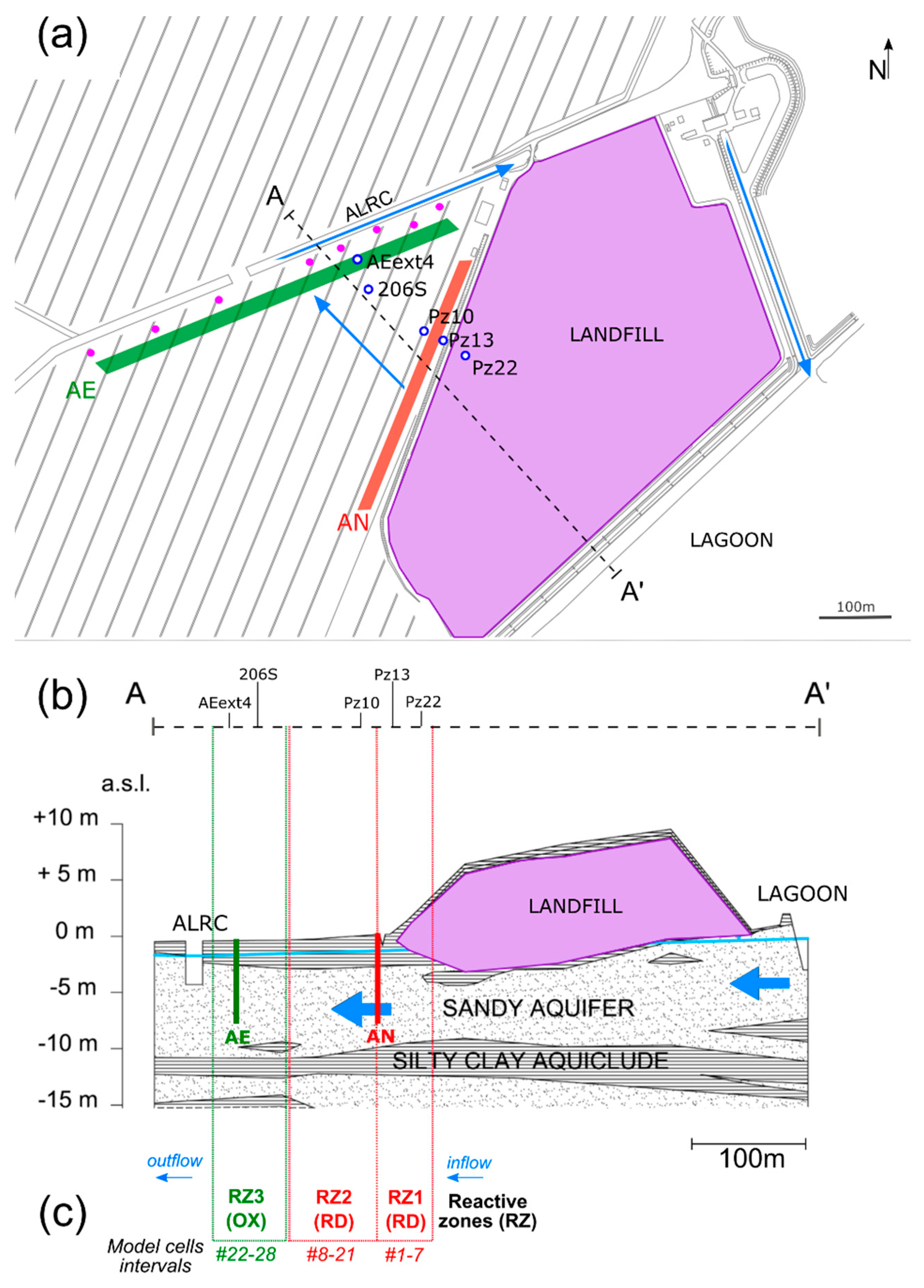
- Pz22 was close to the landfill and far upgradient of the AN and AE barriers. Hence, chloroethenes concentrations and isotopic compositions at Pz22 should be representative of the source conditions.
- Pz13 was located at a distance = 30 m from Pz22, immediately upgradient of the AN barrier and far upgradient of the AE barrier. Hence, chloroethenes at Pz13 should be mainly affected by natural degradation.
- Pz10 was located at = 60 m from Pz22, immediately downgradient of the AN barrier, but upgradient of the AE barrier. Chloroethenes at Pz10 should therefore be affected by anaerobic biostimulation and no aerobic biostimulation was expected here.
- 206S was located at = 164 m from Pz22, further downgradient of the AN barrier and immediately upgradient of the AE one. Here, the transition from RD to OX of chloroethenes took place.
- AEext4 was located at = 200 m from Pz22, downgradient of the AE barrier and upgradient of the P&T wells. Chloroethenes at AEext4 should be mainly affected by OX.
2.3. Geochemical Model
2.3.1. Reaction Network
2.3.2. Reactive Transport Model
- Reactive zone 1 (RZ1), including model cells 1–7 and parametrized by and . It represented the portion of the flow path immediately upgradient of the AN barrier, from Pz22 to between Pz13 and Pz10, where the AN barrier was located. Here, only natural RD was expected to take place without stimulation by the AN barrier.
- Reactive zone 2 (RZ2), including cells 8–21 and parametrized by and . It represented the portion of the flow path located between the AN and AE barriers until just upgradient of the piezometer 206S. Stimulated RD was expected to take place in this section of the flow path.
- Reaction zone 3 (RZ3), including cells 22–28 and parametrized by and . It represented the last portion of the flow path extending from 206S to the end of the transect, which included the AE barrier and piezometer AEext4 just downgradient of it. OX was expected to be largely stimulated by the AE barrier, while RD was not expected to be as efficient as in the upgradient zones.
2.3.3. Model Calibration
3. Results
3.1. Hydrochemical and Isotopic Analyses
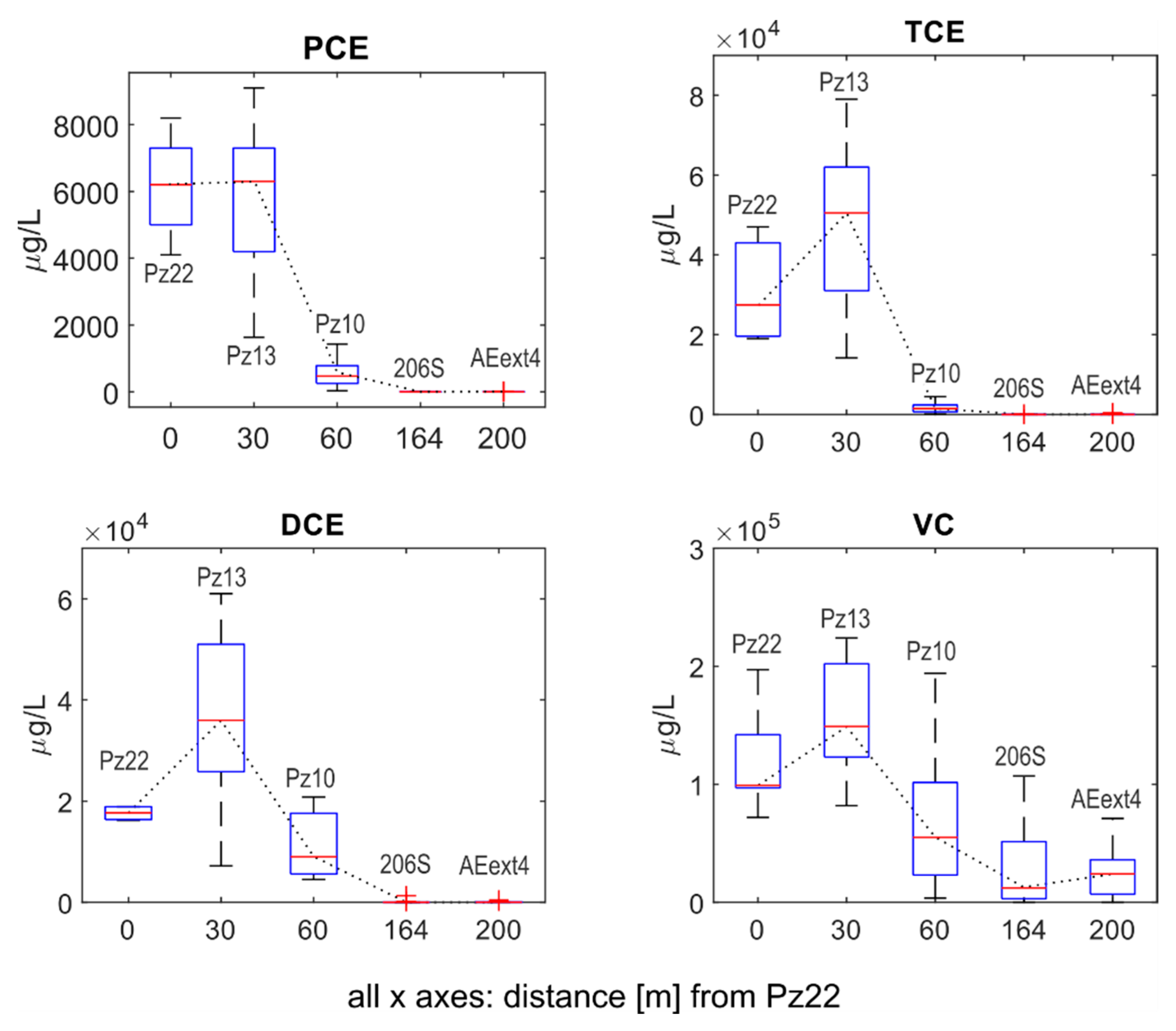
3.1.1. Concentration Data
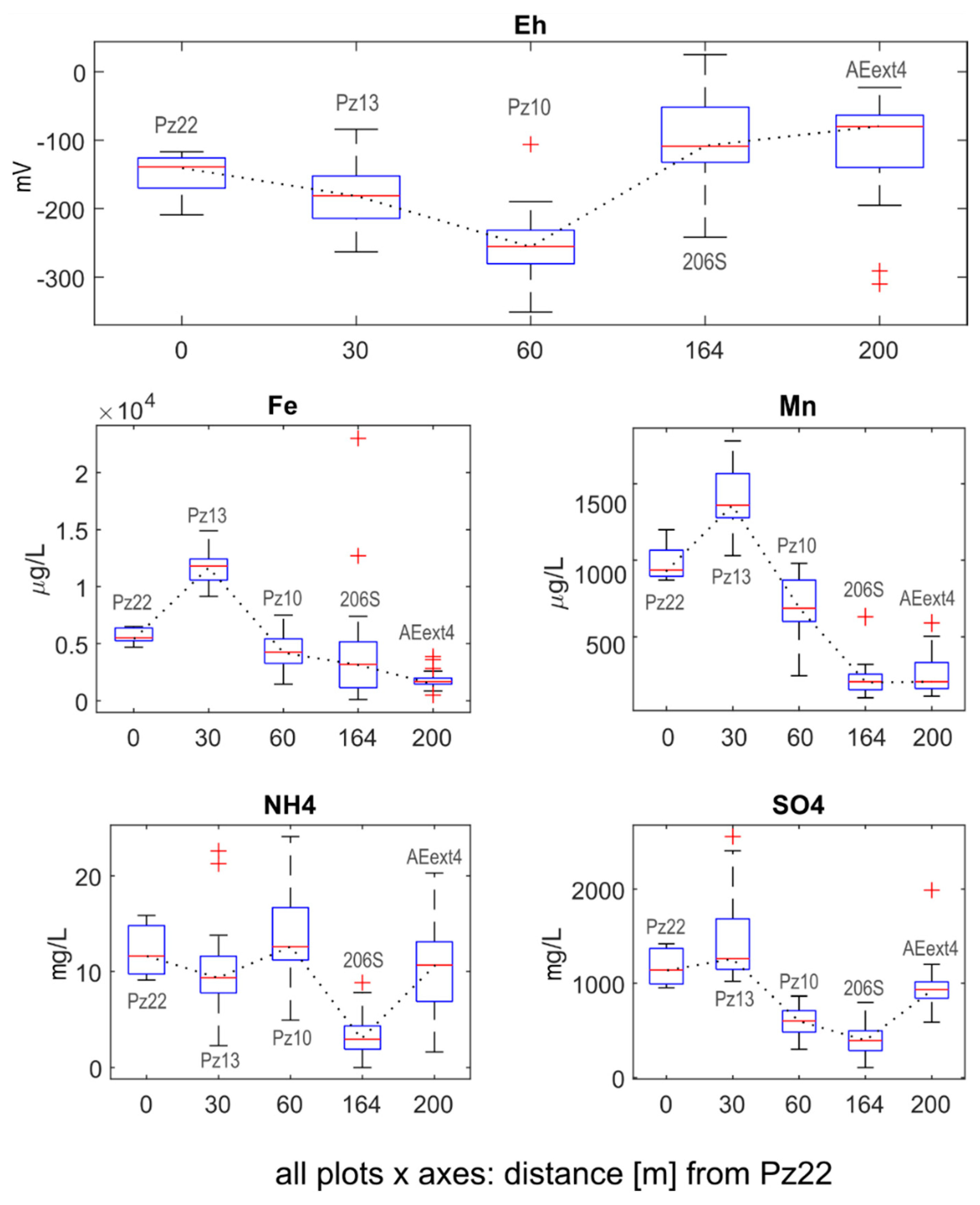
3.1.2. Environmental Parameters
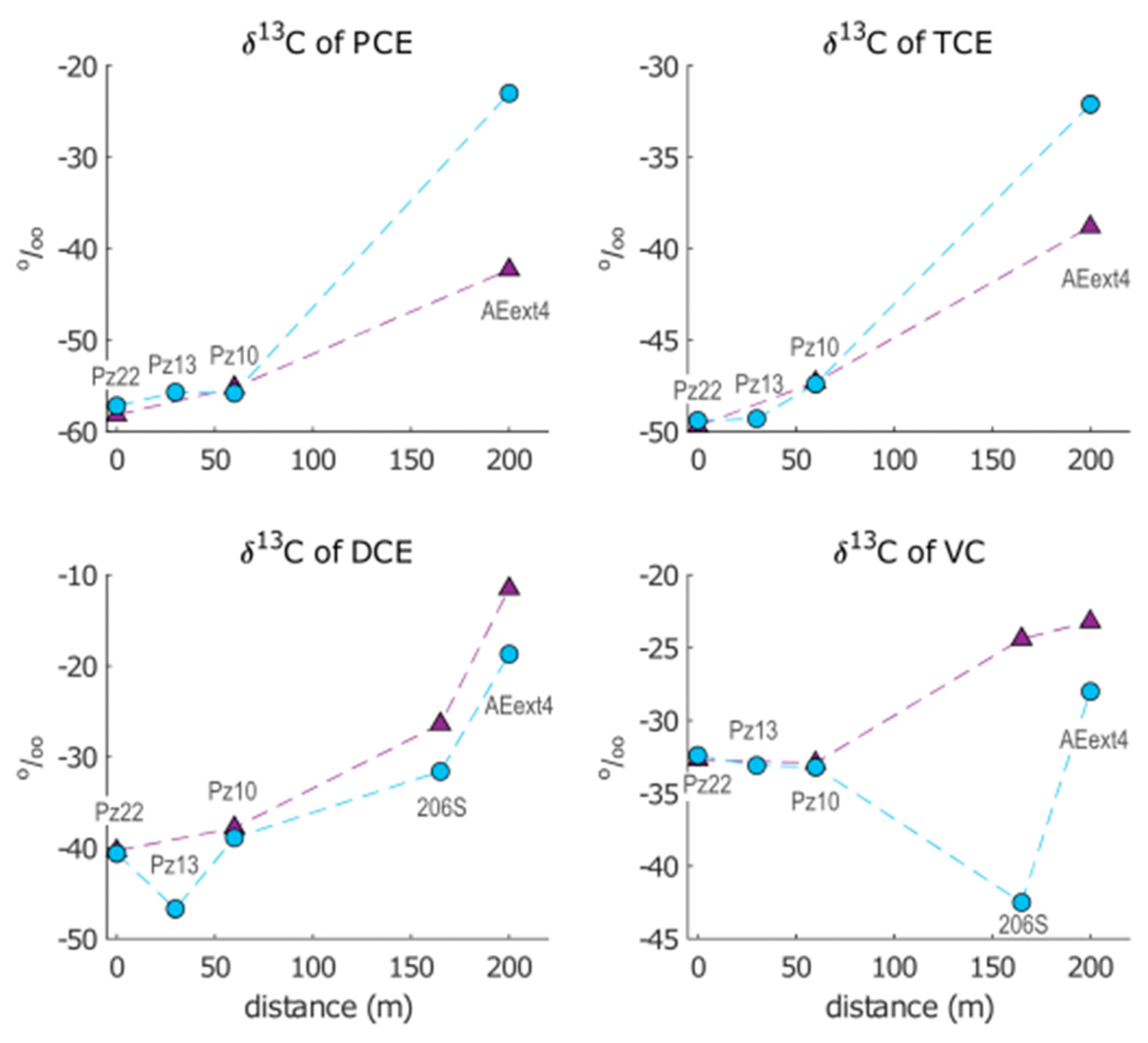
3.1.3. C-CSIA Data
3.2. Geochemical Model
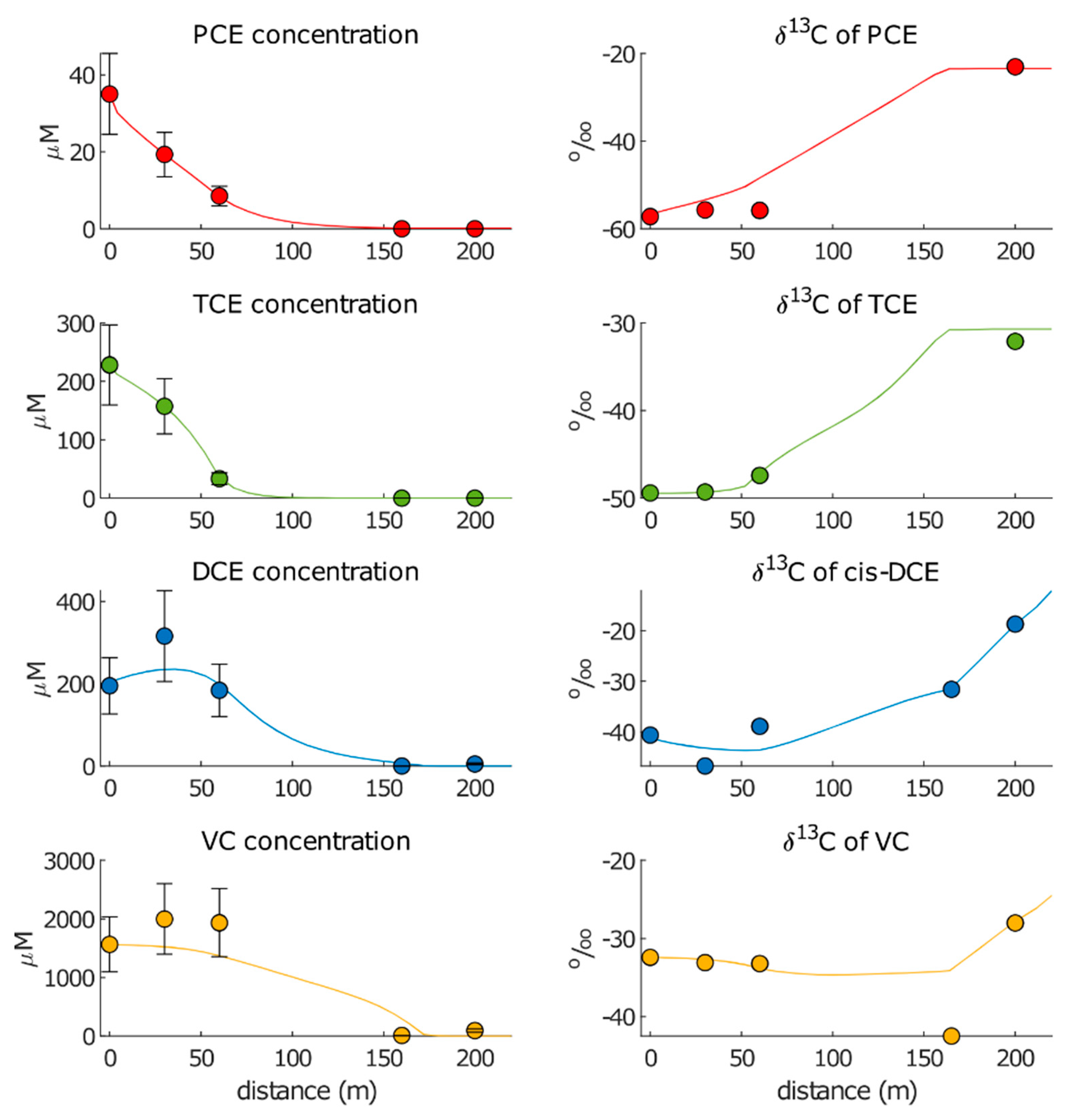
3.2.1. Approach 1
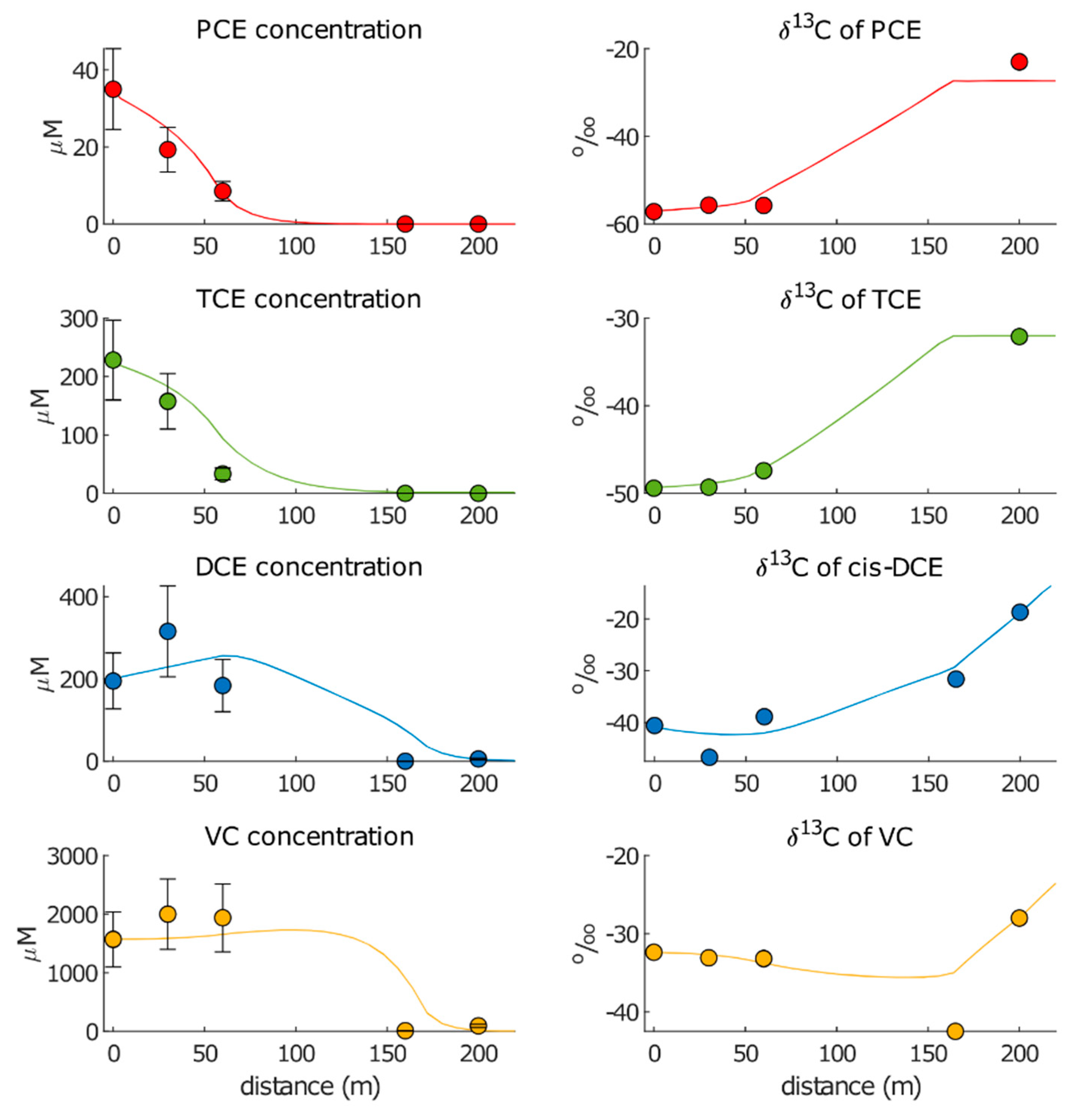
3.2.2. Approach 2
4. Discussion
4.1. Interpretation of the Fitted Parameters in “Approach 2”
4.2. Limitations and Future Developments
5. Conclusions
Supplementary Materials
Author Contributions
Funding
Institutional Review Board Statement
Informed Consent Statement
Data Availability Statement
Acknowledgments
Conflicts of Interest
Abbreviations
| M | Unit of mass |
| L | Unit of length |
| T | Unit of time |
| CSIA | Compound-specific isotope analysis |
| ISB | In situ bioremediation |
| AN | Anaerobic |
| AE | Aerobic |
| PCE | Tetrachloroethene |
| TCE | Trichloroethene |
| DCE | Dichloroethene |
| VC | Vinyl chloride |
| RD | Reductive dechlorination |
| OX | Oxidation |
| ALRC | Artificial land reclamation canal |
| RZ | Reactive zone |
| kOX | Degradation rate constant for OX |
| kRD | Degradation rate constant for RD |
| L | Longitudinal dispersivity |
| Enrichment factor | |
| Retarded velocity | |
| Non-reactive velocity or tracer velocity | |
| Retardation factor | |
| Average retardation factor | |
| Bulk density | |
| Porosity | |
| Fraction of organic carbon | |
| Partition coefficient between organic carbon and water (L/kg or cm3/g) | |
| Distribution coefficient (mg sorbed/kg solid)/(mg solute/L pore water) (L/kg or cm3/g) |
References
- Devlin, J.F.; Katic, D.; Barker, J.F. In Situ Sequenced Bioremediation of Mixed Contaminants in Groundwater. J. Contam. Hydrol. 2004, 69, 233–261. [Google Scholar] [CrossRef]
- Leeson, A.; Beevar, E.; Henry, B.; Fortenberry, J.; Coyle, C. Principles and Practices of Enhanced Anaerobic Bioremediation of Chlorinated Solvents; Naval Facilities Engineering Service Center: Port Hueneme, CA, USA, 2004. [Google Scholar]
- Tiehm, A.; Schmidt, K.R. Sequential Anaerobic/Aerobic Biodegradation of Chloroethenes—Aspects of Field Application. Curr. Opin. Biotechnol. 2011, 22, 415–421. [Google Scholar] [CrossRef] [PubMed]
- Antelmi, M.; Mazzon, P.; Höhener, P.; Marchesi, M.; Alberti, L. Evaluation of MNA in A Chlorinated Solvents-Contaminated Aquifer Using Reactive Transport Modeling Coupled with Isotopic Fractionation Analysis. Water 2021, 13, 2945. [Google Scholar] [CrossRef]
- Thomas, J.M.; Ward, C.H. In Situ Biorestoration of Organic Contaminants in the Subsurface. Environ. Sci. Technol. 1989, 23, 760–766. [Google Scholar] [CrossRef]
- Fralish, M.S.; Downs, J.W. Vinyl Chloride Toxicity. In StatPearls; StatPearls Publishing: Treasure Island, FL, USA, 2022. [Google Scholar]
- Frascari, D.; Fraraccio, S.; Nocentini, M.; Pinelli, D. Aerobic/Anaerobic/Aerobic Sequenced Biodegradation of a Mixture of Chlorinated Ethenes, Ethanes and Methanes in Batch Bioreactors. Bioresour. Technol. 2013, 128, 479–486. [Google Scholar] [CrossRef]
- Němeček, J.; Marková, K.; Špánek, R.; Antoš, V.; Kozubek, P.; Lhotský, O.; Černík, M. Hydrochemical Conditions for Aerobic/Anaerobic Biodegradation of Chlorinated Ethenes—A Multi-Site Assessment. Water 2020, 12, 322. [Google Scholar] [CrossRef]
- Lai, A.; Aulenta, F.; Mingazzini, M.; Palumbo, M.T.; Papini, M.P.; Verdini, R.; Majone, M. Bioelectrochemical Approach for Reductive and Oxidative Dechlorination of Chlorinated Aliphatic Hydrocarbons (CAHs). Chemosphere 2017, 169, 351–360. [Google Scholar] [CrossRef]
- Zheng, C.; Bennett, G.D. Applied Contaminant Transport Modeling, 2nd ed.; John Wiley & Sons: New York, NY, USA, 1997. [Google Scholar]
- Varisco, S.; Beretta, G.P.; Raffaelli, L.; Raimondi, P.; Pedretti, D. Model-Based Analysis of the Link between Groundwater Table Rising and the Formation of Solute Plumes in a Shallow Stratified Aquifer. Pollutants 2021, 1, 66–86. [Google Scholar] [CrossRef]
- Casasso, A.; Tosco, T.; Bianco, C.; Bucci, A.; Sethi, R. How Can We Make Pump and Treat Systems More Energetically Sustainable? Water 2019, 12, 67. [Google Scholar] [CrossRef]
- Ciampi, P.; Esposito, C.; Petrageli Papini, M. Hydrogeochemical Model Supporting the Remediation Strategy of a Highly Contaminated Industrial Site. Water 2019, 11, 1371. [Google Scholar] [CrossRef]
- Van Breukelen, B.M.; Thouement, H.A.A.; Stack, P.E.; Vanderford, M.; Philp, P.; Kuder, T. Modeling 3D-CSIA Data: Carbon, Chlorine, and Hydrogen Isotope Fractionation during Reductive Dechlorination of TCE to Ethene. J. Contam. Hydrol. 2017, 204, 79–89. [Google Scholar] [CrossRef] [PubMed]
- Van Breukelen, B.M.; Hunkeler, D.; Volkering, F. Quantification of Sequential Chlorinated Ethene Degradation by Use of a Reactive Transport Model Incorporating Isotope Fractionation. Environ. Sci. Technol. 2005, 39, 4189–4197. [Google Scholar] [CrossRef] [PubMed]
- Barajas-Rodriguez, F.J.; Murdoch, L.C.; Falta, R.W.; Freedman, D.L. Simulation of in Situ Biodegradation of 1,4-Dioxane under Metabolic and Cometabolic Conditions. J. Contam. Hydrol. 2019, 223, 103464. [Google Scholar] [CrossRef] [PubMed]
- Liu, P.; Wang, G.; Shang, M.; Liu, M. Groundwater Nitrate Bioremediation Simulation of In Situ Horizontal Well by Microbial Denitrification Using PHREEQC. Water. Air. Soil Pollut. 2021, 232, 356. [Google Scholar] [CrossRef]
- Steefel, C.I.; Appelo, C.a.J.; Arora, B.; Jacques, D.; Kalbacher, T.; Kolditz, O.; Lagneau, V.; Lichtner, P.C.; Mayer, K.U.; Meeussen, J.C.L.; et al. Reactive Transport Codes for Subsurface Environmental Simulation. Comput. Geosci. 2014, 19, 445–478. [Google Scholar] [CrossRef]
- Appelo, C.A.J.; Postma, D. Geochemistry, Groundwater and Pollution; A.A. Balkema Publishers: London, UK, 2005. [Google Scholar]
- Pooley, K.E.; Blessing, M.; Schmidt, T.C.; Haderlein, S.B.; MacQuarrie, K.T.B.; Prommer, H. Aerobic Biodegradation of Chlorinated Ethenes in a Fractured Bedrock Aquifer: Quantitative Assessment by Compound-Specific Isotope Analysis (CSIA) and Reactive Transport Modeling. Environ. Sci. Technol. 2009, 43, 7458–7464. [Google Scholar] [CrossRef]
- Courbet, C.; Rivière, A.; Jeannottat, S.; Rinaldi, S.; Hunkeler, D.; Bendjoudi, H.; de Marsily, G. Complementing Approaches to Demonstrate Chlorinated Solvent Biodegradation in a Complex Pollution Plume: Mass Balance, PCR and Compound-Specific Stable Isotope Analysis. J. Contam. Hydrol. 2011, 126, 315–329. [Google Scholar] [CrossRef]
- Casiraghi, G.; Pedretti, D.; Beretta, G.P.; Bertolini, M.; Bozzetto, G.; Cavalca, L.; Ferrari, L.; Masetti, M.; Terrenghi, J. Piloting Activities for the Design of a Large-Scale Biobarrier Involving In Situ Sequential Anaerobic–Aerobic Bioremediation of Organochlorides and Hydrocarbons. Water. Air. Soil Pollut. 2022, 233, 425. [Google Scholar] [CrossRef]
- Dalla Libera, N.; Pedretti, D.; Tateo, F.; Mason, L.; Piccinini, L.; Fabbri, P. Conceptual Model of Arsenic Mobility in the Shallow Alluvial Aquifers near Venice (Italy) Elucidated through Machine Learning and Geochemical Modeling. Water Resour. Res. 2020, 56, e2019WR026234. [Google Scholar] [CrossRef]
- Carraro, A.; Fabbri, P.; Giaretta, A.; Peruzzo, L.; Tateo, F.; Tellini, F. Effects of Redox Conditions on the Control of Arsenic Mobility in Shallow Alluvial Aquifers on the Venetian Plain (Italy). Sci. Total Environ. 2015, 532, 581–594. [Google Scholar] [CrossRef]
- Beretta, G.P.; Terrenghi, J. Groundwater Flow in the Venice Lagoon and Remediation of the Porto Marghera Industrial Area (Italy). Hydrogeol. J. 2017, 25, 847–861. [Google Scholar] [CrossRef]
- Holliger, C.; Wohlfarth, G.; Diekert, G. Reductive Dechlorination in the Energy Metabolism of Anaerobic Bacteria. FEMS Microbiol. Rev. 1998, 22, 383–398. [Google Scholar] [CrossRef]
- Lee, I.-S.; Bae, J.-H.; Yang, Y.; McCarty, P.L. Simulated and Experimental Evaluation of Factors Affecting the Rate and Extent of Reductive Dehalogenation of Chloroethenes with Glucose. J. Contam. Hydrol. 2004, 74, 313–331. [Google Scholar] [CrossRef] [PubMed]
- Bouwer, E.; Norris, R.; Hinchee, R.; Brown, R.A.; Semprini, L.; Wilson, J.T.; Kampbell, D.H.; Reinhard, M.; Borden, R.C.; Vogel, T.; et al. Bioremediation of Chlorinated Solvents Using Alternate Electron Acceptors. In Hanbook Bioremediation; CRC Press: Boca Raton, FL, USA, 1994; pp. 149–175. [Google Scholar]
- Parkhurst, D.L.; Appelo, C.A.J. Description of Input and Examples for PHREEQC Version 3—A Computer Program for Speciation, Batch-Reaction, One-Dimensional Transport, and Inverse Geochemical Calculations; U.S. Geological Survey: Denver, CO, USA, 2013; p. 493. [Google Scholar]
- Dolinová, I.; Štrojsová, M.; Černík, M.; Němeček, J.; Macháčková, J.; Ševců, A. Microbial Degradation of Chloroethenes: A Review. Environ. Sci. Pollut. Res. 2017, 24, 13262–13283. [Google Scholar] [CrossRef] [PubMed]
- Craig, H. Isotopic Standards for Carbon and Oxygen and Correction Factors for Mass-Spectrometric Analysis of Carbon Dioxide. Geochim. Cosmochim. Acta 1957, 12, 133–149. [Google Scholar] [CrossRef]
- Tillotson, J.M.; Borden, R.C. Rate and Extent of Chlorinated Ethene Removal at 37 ERD Sites. J. Environ. Eng. 2017, 143, 04017028. [Google Scholar] [CrossRef]
- Suarez, M.P.; Rifai, H.S. Biodegradation Rates for Fuel Hydrocarbons and Chlorinated Solvents in Groundwater. Bioremediat. J. 1999, 3, 337–362. [Google Scholar] [CrossRef]
- ESTCP Project ER-201029. Environmental Security and Technology Certification Program, Arlington, Virginia; Report; 2014; p. 244. Available online: https://clu-in.org/download/contaminantfocus/tce/ER-201029-User-Guide.pdf (accessed on 20 October 2022).
- Domenico, P.; Schwartz, F.W. Physical and Chemical Hydrogeology; John Wiley & Sons, Inc.: Hoboken, NJ, USA, 1990; ISBN 978-0-471-59762-9. [Google Scholar]
- Gelhar, L.W.; Welty, C.; Rehfeldt, K.R. A Critical Review of Data on Field-Scale Dispersion in Aquifers. Water Resour. Res. 1992, 28, 1955–1974. [Google Scholar] [CrossRef]
- Freeze, R.A.; Cherry, J.A. Groundwater; Prentice-Hall: Englewood Cliffs, NJ, USA, 1979. [Google Scholar]
- Terrenghi, J. Flusso Idrico E Trasporto Reattivo Di Contaminanti In Acquiferi Eterogenei E Applicazioni. PhD Thesis, Università degli Studi di Milano, Milan, Italy, 2018. (In Italian). [Google Scholar] [CrossRef]
- ISS-INAIL ISS-INAIL Database for Environmental Health Risk Analysis. Online Database. Available online: https://www.isprambiente.gov.it/it/attivita/suolo-e-territorio/siti-contaminati/analisi-di-rischio (accessed on 1 May 2022). (In Italian)
- Christensen, T.H.; Bjerg, P.L.; Banwart, S.A.; Jakobsen, R.; Heron, G.; Albrechtsen, H.-J. Characterization of Redox Conditions in Groundwater Contaminant Plumes. J. Contam. Hydrol. 2000, 45, 165–241. [Google Scholar] [CrossRef]
- Hyun, S.P.; Hayes, K.F. Feasibility of Using In Situ FeS Precipitation for TCE Degradation. J. Environ. Eng. 2009, 135, 1009–1014. [Google Scholar] [CrossRef]
- D’Affonseca, F.M.; Prommer, H.; Finkel, M.; Blum, P.; Grathwohl, P. Modeling the Long-Term and Transient Evolution of Biogeochemical and Isotopic Signatures in Coal Tar-Contaminated Aquifers: Modeling Coal Tar-Contaminated Aquifers. Water Resour. Res. 2011, 47, 22. [Google Scholar] [CrossRef]
- He, Y.T.; Wilson, J.T.; Su, C.; Wilkin, R.T. Review of Abiotic Degradation of Chlorinated Solvents by Reactive Iron Minerals in Aquifers. Groundw. Monit. Remediat. 2015, 35, 57–75. [Google Scholar] [CrossRef]
- Dalla Libera, N.; Fabbri, P.; Mason, L.; Piccinini, L.; Pola, M. A Local Natural Background Level Concept to Improve the Natural Background Level: A Case Study on the Drainage Basin of the Venetian Lagoon in Northeastern Italy. Environ. Earth Sci. 2018, 77, 487. [Google Scholar] [CrossRef]
- Slater, G.F.; Sherwood Lollar, B.; Sleep, B.E.; Edwards, E.A. Variability in Carbon Isotopic Fractionation during Biodegradation of Chlorinated Ethenes: Implications for Field Applications. Environ. Sci. Technol. 2001, 35, 901–907. [Google Scholar] [CrossRef]
- Cichocka, D.; Siegert, M.; Imfeld, G.; Andert, J.; Beck, K.; Diekert, G.; Richnow, H.-H.; Nijenhuis, I. Factors Controlling the Carbon Isotope Fractionation of Tetra- and Trichloroethene during Reductive Dechlorination by Sulfurospirillum Ssp. and Desulfitobacterium Sp. Strain PCE-S: Carbon Isotope Fractionation during Reductive Dechlorination. FEMS Microbiol. Ecol. 2007, 62, 98–107. [Google Scholar] [CrossRef]
- Liang, X.; Dong, Y.; Kuder, T.; Krumholz, L.R.; Philp, R.P.; Butler, E.C. Distinguishing Abiotic and Biotic Transformation of Tetrachloroethylene and Trichloroethylene by Stable Carbon Isotope Fractionation. Environ. Sci. Technol. 2007, 41, 7094–7100. [Google Scholar] [CrossRef]
- Wiegert, C.; Mandalakis, M.; Knowles, T.; Polymenakou, P.N.; Aeppli, C.; Macháčková, J.; Holmstrand, H.; Evershed, R.P.; Pancost, R.D.; Gustafsson, Ö. Carbon and Chlorine Isotope Fractionation During Microbial Degradation of Tetra- and Trichloroethene. Environ. Sci. Technol. 2013, 47, 6449–6456. [Google Scholar] [CrossRef]
- Renpenning, J.; Hitzfeld, K.L.; Gilevska, T.; Nijenhuis, I.; Gehre, M.; Richnow, H.-H. Development and Validation of an Universal Interface for Compound-Specific Stable Isotope Analysis of Chlorine (37 Cl/ 35 Cl) by GC-High-Temperature Conversion (HTC)-MS/IRMS. Anal. Chem. 2015, 87, 2832–2839. [Google Scholar] [CrossRef]
- Hourbron, E.; Escoffier, S.; Capdeville, B. Trichloroethylene Elimination Assay by Naural Consortia of Heterotrophic and Methanotrophic Bacteria. Water Sci. Technol. 2000, 42, 395–402. [Google Scholar] [CrossRef]
- Powell, C.L.; Goltz, M.N.; Agrawal, A. Degradation Kinetics of Chlorinated Aliphatic Hydrocarbons by Methane Oxidizers Naturally-Associated with Wetland Plant Roots. J. Contam. Hydrol. 2014, 170, 68–75. [Google Scholar] [CrossRef]
- Zalesak, M.; Ruzicka, J.; Vicha, R.; Dvorackova, M. Cometabolic Degradation of Dichloroethenes by Comamonas Testosteroni RF2. Chemosphere 2017, 186, 919–927. [Google Scholar] [CrossRef] [PubMed]
- Wang, C.-C.; Li, C.-H.; Yang, C.-F. Acclimated Methanotrophic Consortia for Aerobic Co-Metabolism of Trichloroethene with Methane. Int. Biodeterior. Biodegrad. 2019, 142, 52–57. [Google Scholar] [CrossRef]
- Ryoo, D.; Shim, H.; Canada, K.; Barbieri, P.; Wood, T.K. Aerobic Degradation of Tetrachloroethylene by Toluene-o-Xylene Monooxygenase of Pseudomonas Stutzeri OX1. Nat. Biotechnol. 2000, 18, 775–778. [Google Scholar] [CrossRef]
- Zimmermann, J.; Halloran, L.J.S.; Hunkeler, D. Tracking Chlorinated Contaminants in the Subsurface Using Compound-Specific Chlorine Isotope Analysis: A Review of Principles, Current Challenges and Applications. Chemosphere 2020, 244, 125476. [Google Scholar] [CrossRef] [PubMed]
- Huang, L.; Sturchio, N.C.; Abrajano, T.; Heraty, L.J.; Holt, B.D. Carbon and Chlorine Isotope Fractionation of Chlorinated Aliphatic Hydrocarbons by Evaporation. Org. Geochem. 1999, 30, 777–785. [Google Scholar] [CrossRef]
- Poulson, S.R.; Drever, J.I. Stable Isotope (C, Cl, and H) Fractionation during Vaporization of Trichloroethylene. Environ. Sci. Technol. 1999, 33, 3689–3694. [Google Scholar] [CrossRef]
- Jeannottat, S.; Hunkeler, D. Chlorine and Carbon Isotopes Fractionation during Volatilization and Diffusive Transport of Trichloroethene in the Unsaturated Zone. Environ. Sci. Technol. 2012, 46, 3169–3176. [Google Scholar] [CrossRef]
- Chapelle, F.H.; Haack, S.K.; Adriaens, P.; Henry, M.A.; Bradley, P.M. Comparison of E h and H 2 Measurements for Delineating Redox Processes in a Contaminated Aquifer. Environ. Sci. Technol. 1996, 30, 3565–3569. [Google Scholar] [CrossRef]
- Kouznetsova, I.; Mao, X.; Robinson, C.; Barry, D.A.; Gerhard, J.I.; McCarty, P.L. Biological Reduction of Chlorinated Solvents: Batch-Scale Geochemical Modeling. Adv. Water Resour. 2010, 33, 969–986. [Google Scholar] [CrossRef]
- Maillard, J.; Schumacher, W.; Vazquez, F.; Regeard, C.; Hagen, W.R.; Holliger, C. Characterization of the Corrinoid Iron-Sulfur ProteinTetrachloroethene Reductive Dehalogenase of Dehalobacterrestrictus. Appl. Environ. Microbiol. 2003, 69, 4628–4638. [Google Scholar] [CrossRef]
- Yu, S.; Semprini, L. Kinetics and Modeling of Reductive Dechlorination at High PCE and TCE Concentrations. Biotechnol. Bioeng. 2004, 88, 451–464. [Google Scholar] [CrossRef] [PubMed]
- Amos, B.K.; Christ, J.A.; Abriola, L.M.; Pennell, K.D.; Löffler, F.E. Experimental Evaluation and Mathematical Modeling of Microbially Enhanced Tetrachloroethene (PCE) Dissolution. Environ. Sci. Technol. 2007, 41, 963–970. [Google Scholar] [CrossRef] [PubMed]
- Cupples, A.M.; Spormann, A.M.; McCarty, P.L. Comparative Evaluation of Chloroethene Dechlorination to Ethene by Dehalococcoides -like Microorganisms. Environ. Sci. Technol. 2004, 38, 4768–4774. [Google Scholar] [CrossRef]
- Widdowson, M.A. Modeling Natural Attenuation of Chlorinated Ethenes Under Spatially Varying Redox Conditions. Biodegradation 2004, 15, 435–451. [Google Scholar] [CrossRef]
- Yu, S.; Dolan, M.E.; Semprini, L. Kinetics and Inhibition of Reductive Dechlorination of Chlorinated Ethylenes by Two Different Mixed Cultures. Environ. Sci. Technol. 2005, 39, 195–205. [Google Scholar] [CrossRef] [PubMed]
- van Warmerdam, E.M.; Frape, S.K.; Aravena, R.; Drimmie, R.J.; Flatt, H.; Cherry, J.A. Stable Chlorine and Carbon Isotope Measurements of Selected Chlorinated Organic Solvents. Appl. Geochem. 1995, 10, 547–552. [Google Scholar] [CrossRef]
- Abe, Y.; Aravena, R.; Zopfi, J.; Shouakar-Stash, O.; Cox, E.; Roberts, J.D.; Hunkeler, D. Carbon and Chlorine Isotope Fractionation during Aerobic Oxidation and Reductive Dechlorination of Vinyl Chloride and Cis-1,2-Dichloroethene. Environ. Sci. Technol. 2009, 43, 101–107. [Google Scholar] [CrossRef]
- Kuder, T.; Philp, P.; Van Breukelen, B.; Thouement, H.A.A.; Vanderford, M.; Newell, C.J. Integrated Stable Isotope—Reactive Transport Model Approach for Assessment of Chlorinated Solvent Degradation. Technical Report, 2014. [Google Scholar]


| PCE | TCE | Cis-DCE | VC | |
|---|---|---|---|---|
| Reductive Dechlorination (RD) | ||||
| min (‰) | −7.12 | −16.40 | −30.50 | −28.80 |
| mean (‰) | −4.51 | −11.65 | −21.43 | −24.52 |
| max (‰) | −1.60 | −3.30 | −14.90 | −19.90 |
| min (y−1) | 0.00 | 0.00 | 0.00 | 0.00 |
| mean (y−1) | 1.07 | 1.10 | 1.82 | 2.20 |
| max (y−1) | 29.00 | 8.40 | 28.00 | 3.00 |
| Oxidation (OX) | ||||
| min (‰) | −19.90 | −8.20 | ||
| mean (‰) | −7.99 | −6.06 | ||
| max (‰) | −0.90 | −3.20 | ||
| min (y−1) | 102.57 | 15.70 | ||
| mean (y−1) | 323.03 | 43.80 | ||
| max (y−1) | 715.40 | 204.40 | ||
| Parameter | Value | Unit |
|---|---|---|
| ) | 224 | m |
| 0.45 | m d−1 | |
| ) | 0.10 | m d−1 |
| ) | 22.4 | m |
| 8 | m | |
| Number of cells | 28 | - |
| Shifts | 50 | - |
| Time step length | 80 | d |
| Equivalent simulation time | 4000 | d |
| Cell numbers for reactive zone 1 | 1–7 | - |
| Cell numbers for reactive zone 2 | 8–21 | - |
| Cell numbers for reactive zone 3 | 22–28 | - |
| Flow inlet/outlet boundary conditions | Constant flux | - |
| Bulk density (ρb) | 1.6 | g cm−3 |
| 0.25 | - | |
| Fraction of organic carbon (foc) | 10% of TOC | - |
| Chloroethene | koc (cm3/g) | ||
|---|---|---|---|
| PCE | 94.94 | 7.08 | 4.47 |
| TCE | 60.70 | 4.88 | |
| Cis-DCE | 39.60 | 3.53 | |
| VC | 21.73 | 2.39 |
| Compound | Concentrations (µM) | δ13C (‰) |
|---|---|---|
| PCE tot | 34.982 | −58.2 ± 0.7 |
| PCE(l) | 34.615 | |
| PCE(h) | 0.367 | |
| TCE tot | 228.137 | −49.7 ± 0.3 |
| TCE(l) | 225.726 | |
| TCE(h) | 2.411 | |
| Cis-DCE tot | 194.845 | −40.3 ± 0.2 |
| Cis-DCE(l) | 192.767 | |
| Cis-DCE(h) | 2.078 | |
| VC tot | 1568.000 | −32.7 ± 0.1 |
| VC(l) | 1551.135 | |
| VC(h) | 16.865 |
| Pz22 | Pz13 | Pz10 | 206s | AEext4 | ||||||
|---|---|---|---|---|---|---|---|---|---|---|
| Conc (µg/L) | δ13C (‰) | Conc (µg/L) | δ13C (‰) | Conc (µg/L) | δ13C (‰) | Conc (µg/L) | δ13C (‰) | Conc (µg/L) | δ13C (‰) | |
| January 2021 | ||||||||||
| PCE | / | −58.2 ± 0.7 | / | / | 1340 | −55.2 ± 0.5 | 0.091 | b.d.l. * | 1.94 | −42.3 ± 0.1 |
| TCE | / | −49.7 ± 0.3 | / | / | 2250 | −47.3 ± 0.1 | 0.41 | b.d.l. * | 8.1 | −38.8 ± 0.6 |
| Cis-DCE | / | −40.3 ± 0.2 | / | / | 17,600 | −37.8 ± 0.2 | 0.71 | −26.4 ± 0.4 | 232 | −11.5 ± 0.5 |
| VC | / | −32.7 ± 0.1 | / | / | 108,000 | −32.9 ± 0.2 | 5200 | −24.4 ± 0.1 | 8000 | −23.2 ± 0.1 |
| May 2021 | ||||||||||
| PCE | 5800 | −57.2 ± 0.3 | 3200 | −55.7 ± 0.1 | 1410 | −55.8 ± 0.4 | 0.054 | / | 0.94 | −23.0 ± 0.5 |
| TCE | 30,000 | −49.4 ± 0.2 | 20,700 | −49.3 ± 0.3 | 4400 | −47.4 ± 0.4 | 0.122 | / | 3.00 | −32.1 ± 0.7 |
| Cis-DCE | 18,900 | −40.6 ± 0.5 | 30,600 | −46.7 ± 0.1 | 17,800 | −38.9 ± 0.5 | 0.5 | −31.6 ± 0.8 | 490 | −18.7 ± 0.5 |
| VC | 98,000 | −32.4 ± 0.3 | 125,000 | −33.1 ± 0.2 | 121,000 | −33.2 ± 0.1 | 590 | −42.5 ± 0.2 | 5800 | −28.0 ± 0.1 |
| PCE | TCE | Cis-DCE | VC | |
|---|---|---|---|---|
| Approach 1—Reductive Dechlorination (RD) | ||||
| kRD1 (y−1) | 0.84 | 0.43 | 0.00 | 0.00 |
| kRD2 (y−1) | 2.70 | 11.00 | 2.15 | 0.48 |
| εRD (‰) | −9.4 | −3.6 | −6.2 | −2.0 |
| Approach 1—Oxidation (OX) | ||||
| kOX (y−1) | - | - | 50 | 50 |
| εOX (‰) | - | - | −2.2 | −1.2 |
| wRMSE | ||||
| Concentrations | 0.07 | 0.60 | 16.60 | 159.50 |
| CSIA | 3.89 | 0.36 | 1.18 | 1.67 |
| Approach 2—Reductive dechlorination (RD) | ||||
| kRD1 (y−1) | 0.3 | 0.2 | 0 | 0 |
| kRD2 (y−1) | 6.5 | 2.9 | 0.6 | 0 |
| εRD (‰) | −5.6 | −5.7 | −16.0 | 0 |
| Approach 2—Oxidation (OX) Using the Average [Minimum ÷ Maximum] εOX | ||||
| kOX (y−1) | - | - | 4.7 [0.7 ÷ 155] | 2.9 [1.7 ÷ 12.6] |
| εOX (‰) | - | - | −7.99 [−19.9 ÷ −0.9] | −6.06 [−8.2 ÷ −3.2] |
| wRMSE (average εOX) | ||||
| Concentrations | 1.10 | 13.14 | 24.08 | 157.76 |
| CSIA | 1.88 | 0.13 | 1.12 | 0.80 |
Publisher’s Note: MDPI stays neutral with regard to jurisdictional claims in published maps and institutional affiliations. |
© 2022 by the authors. Licensee MDPI, Basel, Switzerland. This article is an open access article distributed under the terms and conditions of the Creative Commons Attribution (CC BY) license (https://creativecommons.org/licenses/by/4.0/).
Share and Cite
Casiraghi, G.; Pedretti, D.; Beretta, G.P.; Masetti, M.; Varisco, S. Assessing a Large-Scale Sequential In Situ Chloroethene Bioremediation System Using Compound-Specific Isotope Analysis (CSIA) and Geochemical Modeling. Pollutants 2022, 2, 462-485. https://doi.org/10.3390/pollutants2040031
Casiraghi G, Pedretti D, Beretta GP, Masetti M, Varisco S. Assessing a Large-Scale Sequential In Situ Chloroethene Bioremediation System Using Compound-Specific Isotope Analysis (CSIA) and Geochemical Modeling. Pollutants. 2022; 2(4):462-485. https://doi.org/10.3390/pollutants2040031
Chicago/Turabian StyleCasiraghi, Giulia, Daniele Pedretti, Giovanni Pietro Beretta, Marco Masetti, and Simone Varisco. 2022. "Assessing a Large-Scale Sequential In Situ Chloroethene Bioremediation System Using Compound-Specific Isotope Analysis (CSIA) and Geochemical Modeling" Pollutants 2, no. 4: 462-485. https://doi.org/10.3390/pollutants2040031
APA StyleCasiraghi, G., Pedretti, D., Beretta, G. P., Masetti, M., & Varisco, S. (2022). Assessing a Large-Scale Sequential In Situ Chloroethene Bioremediation System Using Compound-Specific Isotope Analysis (CSIA) and Geochemical Modeling. Pollutants, 2(4), 462-485. https://doi.org/10.3390/pollutants2040031