
Analysis and Selection of Multiple Machine Learning Methodologies in PyCaret for Monthly Electricity Consumption Demand Forecasting †

 , , and
Abstract
1. Introduction
- To evaluate the performance of 27 machine learning models available in PyCaret for forecasting monthly electricity consumption.
- To identify the three most effective models based on a comprehensive analysis of eight evaluation metrics.
2. Materials and Methods
2.1. Study Area
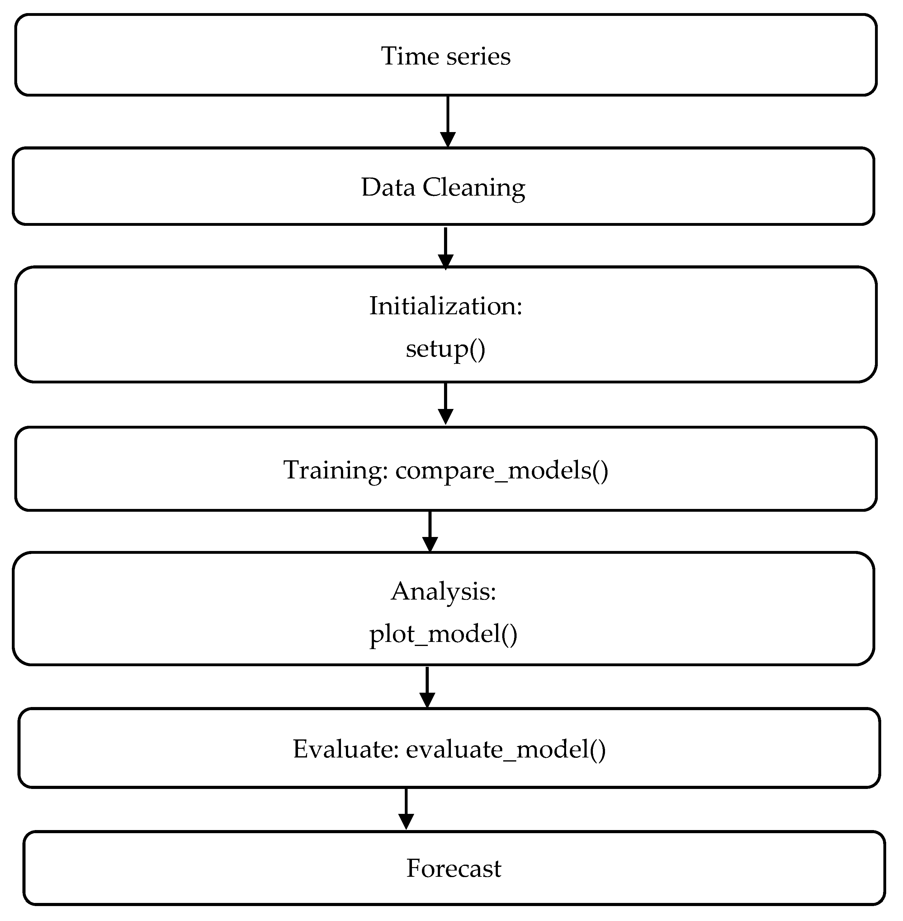
2.2. Methodology
- 3.
- Data Collection: We extracted historical monthly electricity consumption data from electrical yearbooks.
- 4.
- Data Preprocessing: We handled missing values and normalized the data. We also applied seasonal decomposition to understand underlying patterns.
- 5.
- Feature Engineering: We created lag features and rolling statistics to capture temporal dependencies.
- 6.
- Model Selection: Various models were selected, including Exponential Smoothing, Adaptive Boosting with Conditional Deseasonalization and Detrending, and ETS.
- 7.
- Model Training and Tuning: We trained the models using PyCaret and tuned the hyperparameters using GridSearchCV.
- 8.
- Evaluation Metrics: Models were evaluated based on MASE, RMSSE, MAE, RMSE, MAPE, SMAPE, R2, and computation time.
2.2.1. Data
2.2.2. Application of Metrics
- 1.
- Mean Absolute Scaled Error (MASE):
- 2.
- Root Mean Squared Scaled Error (RMSSE):
- 3.
- Mean Absolute Error (MAE):
- 4.
- Root Mean Squared Error (RMSE):
- 5.
- Mean Absolute Percentage Error (MAPE):
- 6.
- Symmetric Mean Absolute Percentage Error (SMAPE):
- 7.
- R2 Comparison:
- 8.
- Computation Time (TT):
3. Results and Discussion
3.1. Data Cleaning and Initialization
3.2. Model Comparison
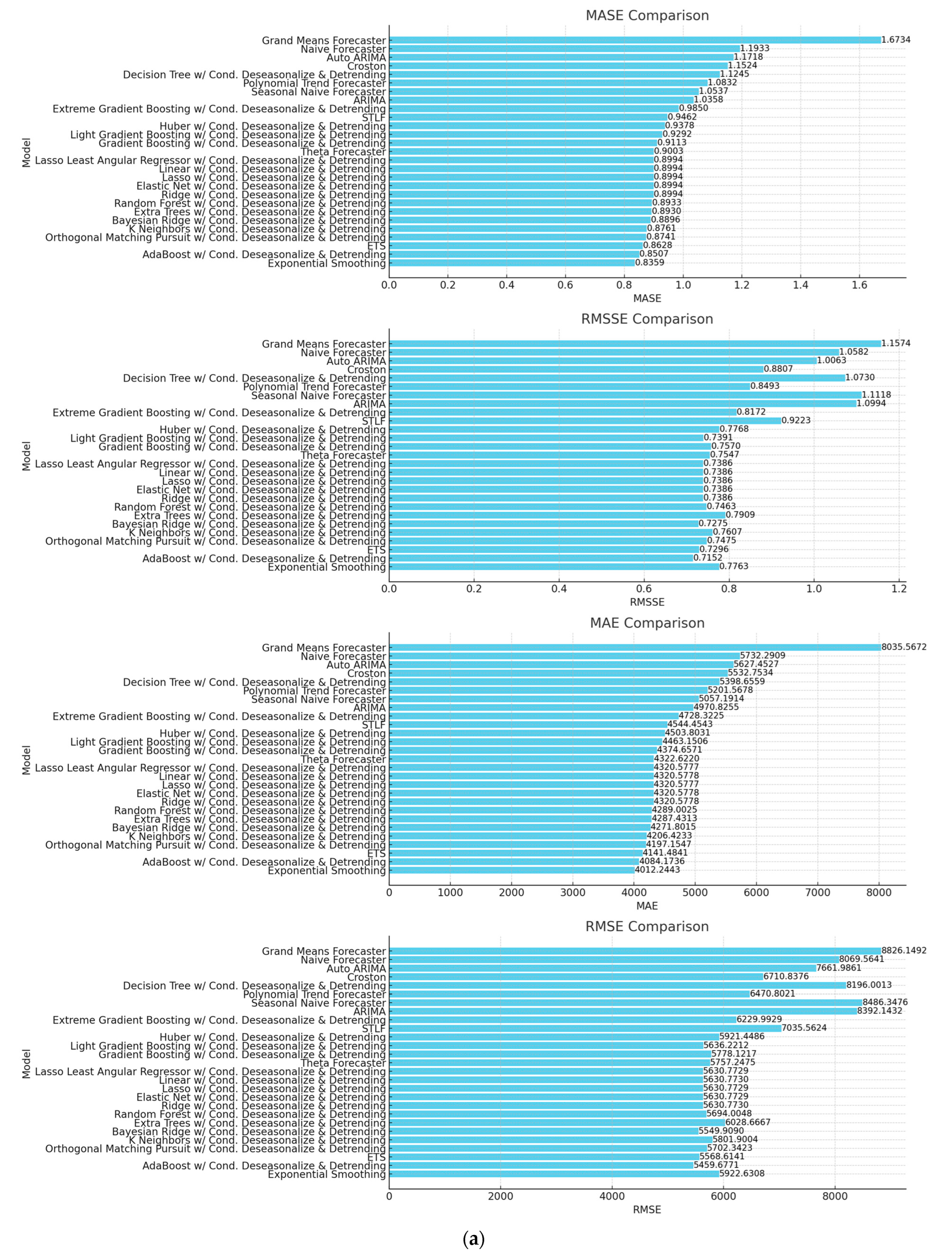
| MASE and RMSSE: |
| Top Models: Exponential Smoothing, AdaBoost with Conditional Deseasonalize and Detrending, ETS. |
| Observation: Exponential Smoothing shows the lowest MASE and RMSSE values, indicating it performs well regarding these error metrics. |
| MAE and RMSE: |
| Top Models: Exponential Smoothing, AdaBoost with Conditional Deseasonalize and Detrending, ETS. |
| Observation: Exponential Smoothing has the lowest MAE and RMSE, making it a strong candidate for minimizing absolute and squared errors. |
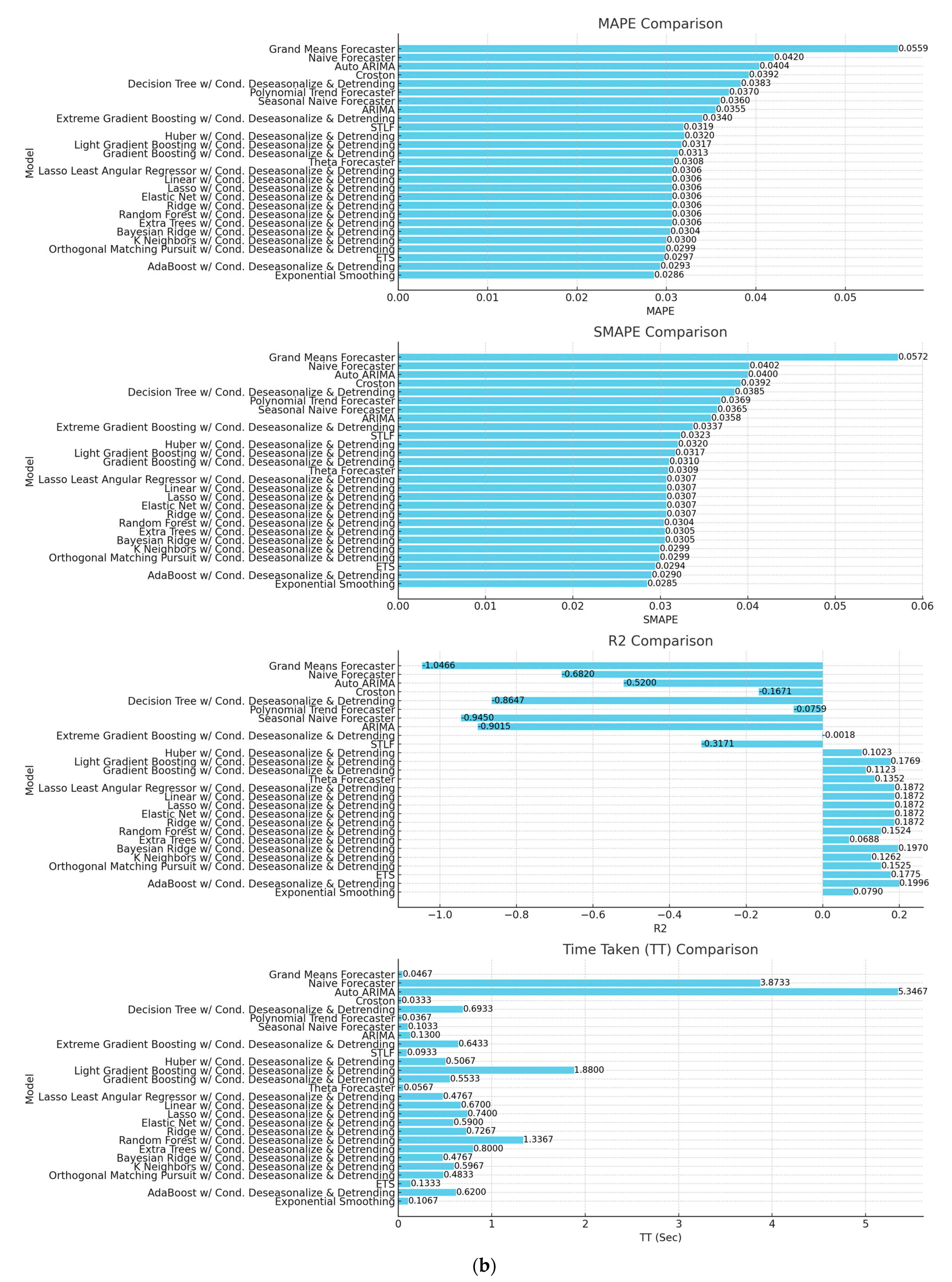
| MAPE and SMAPE: |
| Top Models: Exponential Smoothing, AdaBoost with Conditional Deseasonalize and Detrending, ETS. |
| Observation: These models consistently show lower values for MAPE and SMAPE, indicating better performance in percentage error metrics. |
| R2: |
| Top Models: AdaBoost with Conditional Deseasonalize and Detrending, ETS. |
| Observation: AdaBoost with Conditional Deseasonalize and detrending shows the highest R2 value, indicating that it explains the most variance in the data. |
| TT (Sec): |
| Top Models (Least Time): Exponential Smoothing, ETS. |
| Observation: Exponential Smoothing and ETS are among the fastest models, making them efficient in terms of computation time. |
| Recommendations |
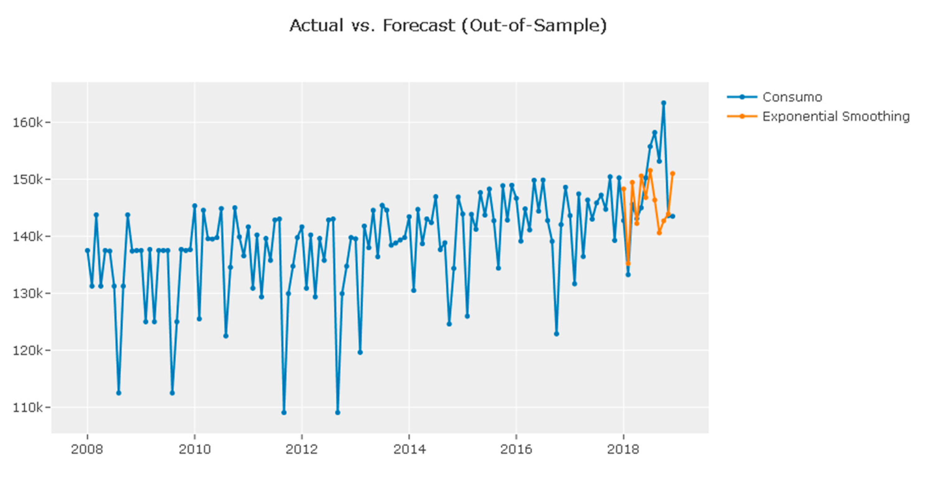
| Best Overall Model: Exponential Smoothing |
| Reason: It consistently performs well across all error metrics and has a low computation time. |
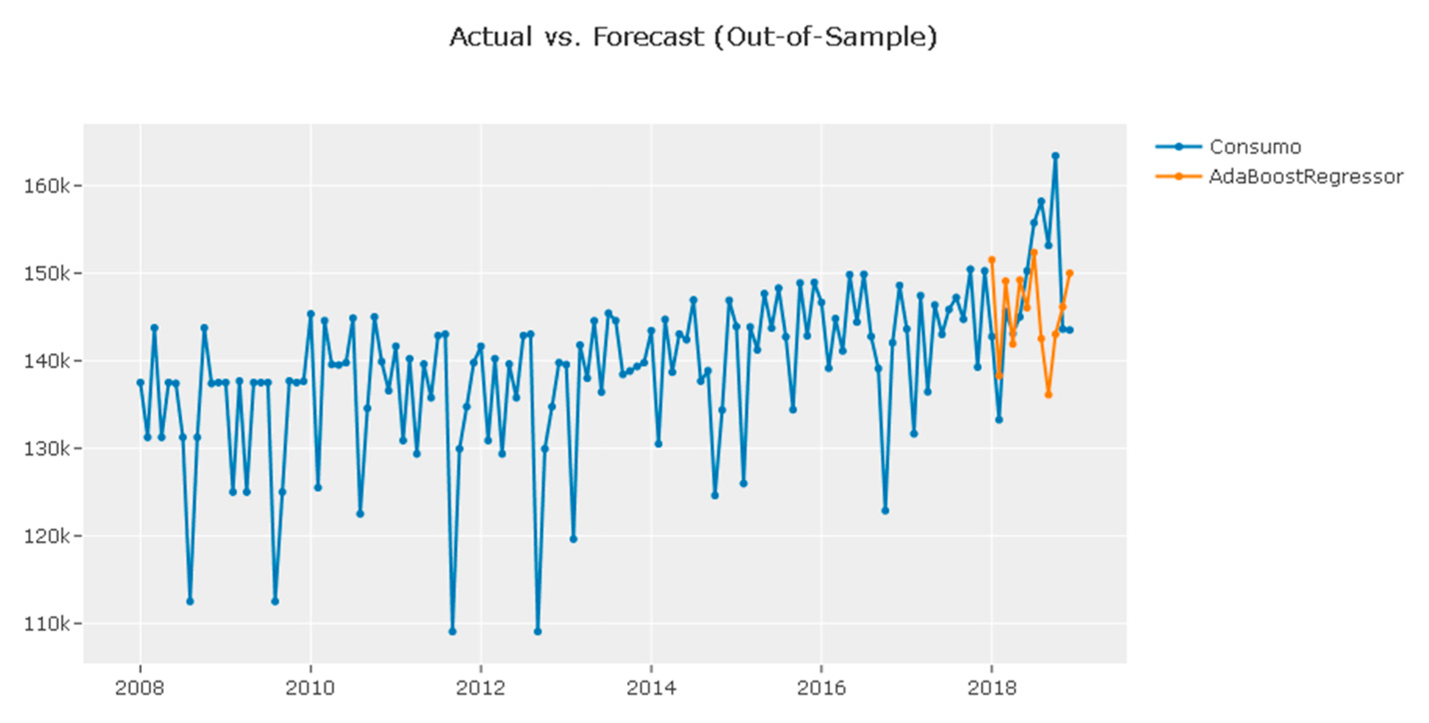
| Runner-Up Models: |
| AdaBoost with Conditional Deseasonalize and Detrending: Shows high R2 and good performance across other metrics. |
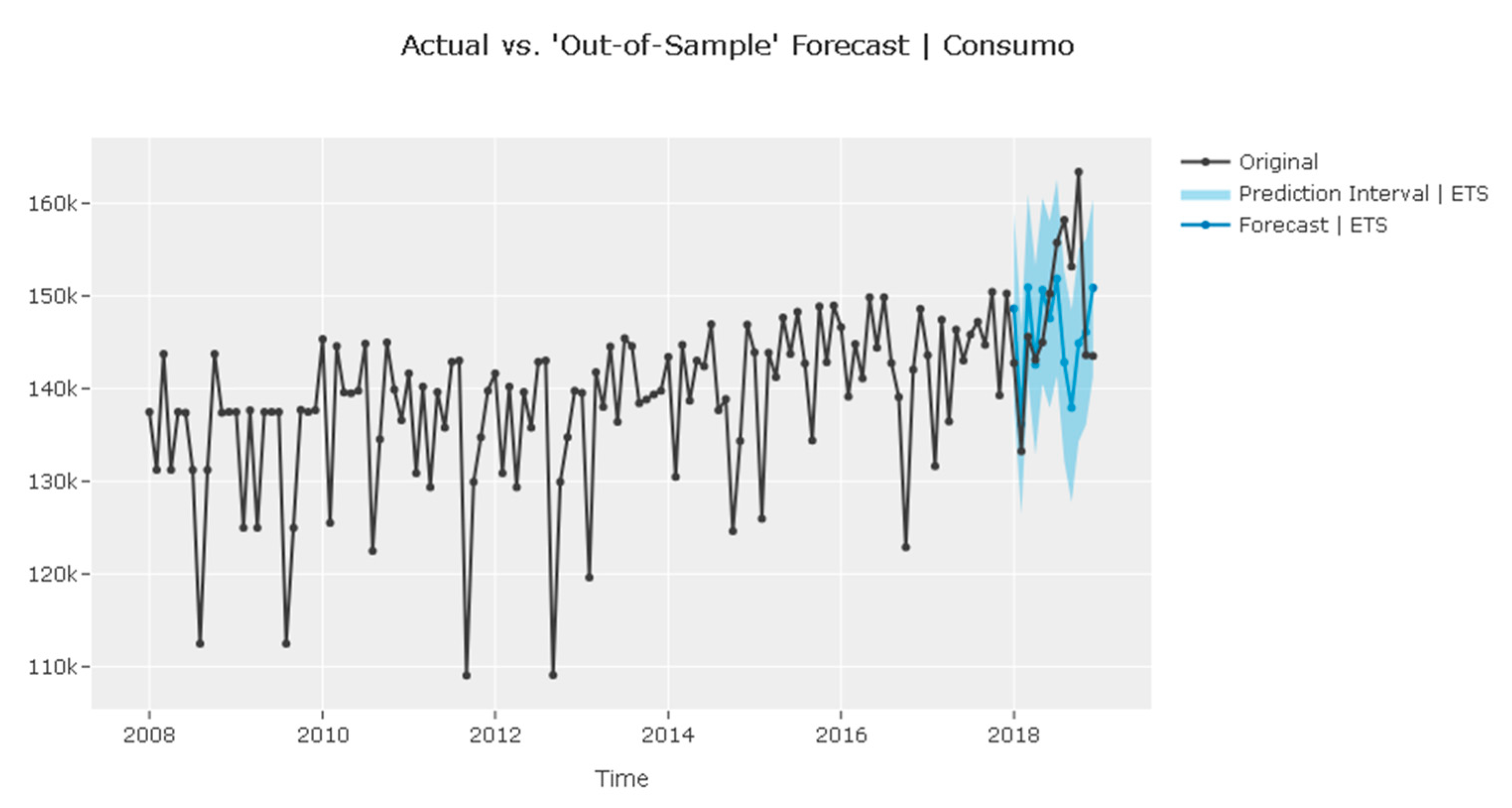
| ETS: Good balance of performance and computation time. |
| We should consider these models for forecasting monthly electricity consumption demand due to their strong performance across multiple metrics and efficiency in computation. |
3.3. Model Creation and Training
3.4. Model Comparison
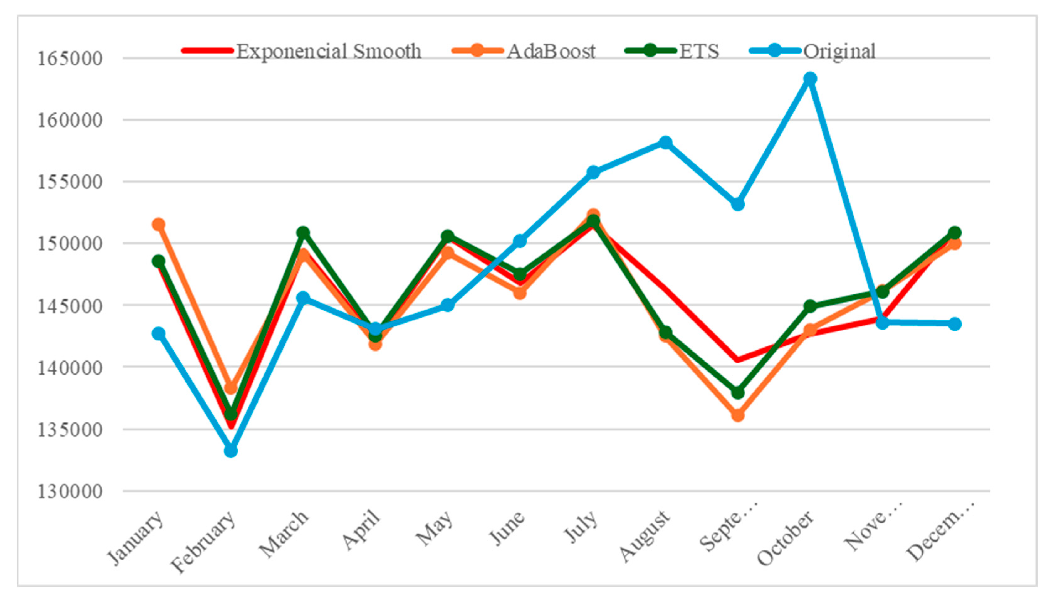
3.5. Forecast Validation
4. Conclusions
Author Contributions
Funding
Institutional Review Board Statement
Informed Consent Statement
Data Availability Statement
Conflicts of Interest
References
- Chong, M.; Aguilar, R. Proyección de Series de Tiempo para el Consumo de la Energía Eléctrica a Clientes Residenciales en Ecuador. Rev. Tecnológica ESPOL-RTE 2016, 29, 56–76. [Google Scholar]
- Mariño, M.D.; Arango, A.; Lotero, L.; Jimenez, M. Modelos de series temporales para pronóstico de la demanda eléctrica del sector de explotación de minas y canteras en Colombia. Rev. EIA 2021, 18, 35007. [Google Scholar] [CrossRef]
- Hyndman, R.J.; Khandakar, Y. Automatic Time Series Forecasting: The forecast Package for R. J. Stat. Softw. 2008, 27, 1–22. [Google Scholar] [CrossRef]
- Manzella, F.; Pagliarini, G.; Sciavicco, G.; Stan, I.E. The voice of COVID-19: Breath and cough recording classification with temporal decision trees and random forests. Artif. Intell. Med. 2023, 137, 102486. [Google Scholar] [CrossRef]
- Ersin, M.; Emre, N.; Eczacioglu, N.; Eker, E.; Yücel, K.; Bekir, H. Enhancing microalgae classification accuracy in marine ecosystems through convolutional neural networks and support vector machines. Mar. Pollut. Bull. 2024, 205, 116616. [Google Scholar] [CrossRef]
- Westergaard, G.; Erden, U.; Mateo, O.A.; Lampo, S.M.; Akinci, T.C.; Topsakal, O. Time Series Forecasting Utilizing Automated Machine Learning (AutoML): A Comparative Analysis Study on Diverse Datasets. Information 2024, 15, 39. [Google Scholar] [CrossRef]
- Arnaut, F.; Kolarski, A.; Srećković, V.A. Machine Learning Classification Workflow and Datasets for Ionospheric VLF Data Exclusion. Data 2024, 9, 17. [Google Scholar] [CrossRef]
- Kilic, K.; Ikeda, H.; Adachi, T.; Kawamura, Y. Soft ground tunnel lithology classification using clustering-guided light gradient boosting machine. J. Rock Mech. Geotech. Eng. 2023, 15, 2857–2867. [Google Scholar] [CrossRef]
- Jose, R.; Syed, F.; Thomas, A.; Toma, M. Cardiovascular Health Management in Diabetic Patients with Machine-Learning-Driven Predictions and Interventions. Appl. Sci. 2024, 14, 2132. [Google Scholar] [CrossRef]
- Effrosynidis, D.; Spiliotis, E.; Sylaios, G.; Arampatzis, A. Time series and regression methods for univariate environmental forecasting: An empirical evaluation. Sci. Total Environ. 2023, 875, 162580. [Google Scholar] [CrossRef]
- Malounas, I.; Lentzou, D.; Xanthopoulos, G.; Fountas, S. Testing the suitability of automated machine learning, hyperspectral imaging and CIELAB color space for proximal in situ fertilization level classification. Smart Agric. Technol. 2024, 8, 100437. [Google Scholar] [CrossRef]
- Gupta, R.; Yadav, A.K.; Jha, S.K.; Pathak, P.K. Long term estimation of global horizontal irradiance using machine learning algorithms. Optik 2023, 283, 170873. [Google Scholar] [CrossRef]
- Arunraj, N.S.; Ahrens, D. A hybrid seasonal autoregressive integrated moving average and quantile regression for daily food sales forecasting. Int. J. Prod. Econ. 2015, 170, 321–335. [Google Scholar] [CrossRef]
- Packwood, D.; Nguyen, L.T.H.; Cesana, P.; Zhang, G.; Staykov, A.; Fukumoto, Y.; Nguyen, D.H. Machine Learning in Materials Chemistry: An Invitation. Mach. Learn. Appl. 2022, 8, 100265. [Google Scholar] [CrossRef]
- Moreno, S.R.; Seman, L.O.; Stefenon, S.F.; dos Santos Coelho, L.; Mariani, V.C. Enhancing wind speed forecasting through synergy of machine learning, singular spectral analysis, and variational mode decomposition. Energy 2024, 292, 130493. [Google Scholar] [CrossRef]
- Slowik, A.; Moldovan, D. Multi-Objective Plum Tree Algorithm and Machine Learning for Heating and Cooling Load Prediction. Energies 2024, 17, 3054. [Google Scholar] [CrossRef]
- Abdu, D.M.; Wei, G.; Yang, W. Assessment of railway bridge pier settlement based on train acceleration response using machine learning algorithms. Structures 2023, 52, 598–608. [Google Scholar] [CrossRef]
- Muqeet, M.; Malik, H.; Panhwar, S.; Khan, I.U.; Hussain, F.; Asghar, Z.; Khatri, Z.; Mahar, R.B. Enhanced cellulose nanofiber mechanical stability through ionic crosslinking and interpretation of adsorption data using machine learning. Int. J. Biol. Macromol. 2023, 237, 124180. [Google Scholar] [CrossRef] [PubMed]
- Xin, L.; Yu, H.; Liu, S.; Ying, G.G.; Chen, C.E. POPs identification using simple low-code machine learning. Sci. Total Environ. 2024, 921, 171143. [Google Scholar] [CrossRef] [PubMed]
- Lynch, C.J.; Gore, R. Application of one-, three-, and seven-day forecasts during early onset on the COVID-19 epidemic dataset using moving average, autoregressive, autoregressive moving average, autoregressive integrated moving average, and naïve forecasting methods. Data Br. 2021, 35, 106759. [Google Scholar] [CrossRef] [PubMed]
- Prestwich, S.D.; Tarim, S.A.; Rossi, R. Intermittency and obsolescence: A Croston method with linear decay. Int. J. Forecast. 2021, 37, 708–715. [Google Scholar] [CrossRef]
- Nguyen, H.V.; Naeem, M.A.; Wichitaksorn, N.; Pears, R. A smart system for short-term price prediction using time series models. Comput. Electr. Eng. 2019, 76, 339–352. [Google Scholar] [CrossRef]
- Adam, M.L.; Moses, O.A.; Mailoa, J.P.; Hsieh, C.Y.; Yu, X.F.; Li, H.; Zhao, H. Navigating materials chemical space to discover new battery electrodes using machine learning. Energy Storage Mater. 2024, 65, 103090. [Google Scholar] [CrossRef]
- Yang, Y.; Yang, Y. Hybrid method for short-term time series forecasting based on EEMD. IEEE Access 2020, 8, 61915–61928. [Google Scholar] [CrossRef]
- Tolios, G. Simplifying Machine Learning with PyCaret A Low-Code Approach for Beginners and Experts! Leanpub: Victoria, BC, Canada, 2022. [Google Scholar]
- Hyndman, R.J.; Athanasopoulos, G. Forecasting: Principles and Practice; OTexts: Melbourne, Australia, 2018. [Google Scholar]
- Freund, Y.; Schapire, R.E. A Decision-Theoretic Generalization of On-Line Learning and an Application to Boosting. J. Comput. Syst. Sci. 1997, 55, 119–139. [Google Scholar] [CrossRef]
- Pati, Y.C.; Rezaiifar, R.; Krishnaprasad, P.S. Orthogonal matching pursuit: Recursive function approximation with applications to wavelet decomposition. In Proceedings of the 27th Asilomar Conference on Signals, Systems and Computers, Pacific Grove, CA, USA, 1–3 November 1993; Volume 1, pp. 40–44. [Google Scholar]
- Fix, E.; Hodges, J.L. Discriminatory Analysis. Nonparametric Discrimination: Consistency Properties. Int. Stat. Rev./Rev. Int. Stat. 1989, 57, 238–247. [Google Scholar] [CrossRef]
- Hoerl, A.E.; Kennard, R.W. Ridge Regression: Biased Estimation for Nonorthogonal Problems. Technometrics 1970, 12, 55–67. [Google Scholar] [CrossRef]
- Geurts, P.; Ernst, D.; Wehenkel, L. Extremely randomized trees. Mach. Learn. 2006, 63, 3–42. [Google Scholar] [CrossRef]
- Breiman, L.; Friedman, J.H.; Olshen, R.A.; Stone, C.J. Classification And Regression Trees, 1st ed.; Routledge: New York, NY, USA, 2017; ISBN 9781315139470. [Google Scholar]
- Tibshirani, R. Regression Shrinkage and Selection via the Lasso. R. Stat. Soc. 1996, 58, 267–288. [Google Scholar] [CrossRef]
- Zou, H.; Hastie, T. Regularization and variable selection via the elastic net. J. R. Stat. Soc. Ser. B Stat. Methodol. 2005, 67, 301–320. [Google Scholar] [CrossRef]
- Draper, N.R.; Smith, H. Applied Regression Analysis, 3rd ed.; John Wiley Sons, Inc.: Hoboken, NJ, USA, 1998. [Google Scholar]
- Efron, B.; Hastie, T.; Johnstone, I.; Tibshirani, R.; Ishwaran, H.; Knight, K.; Loubes, J.M.; Massart, P.; Madigan, D.; Ridgeway, G.; et al. Least angle regression. Ann. Stat. 2004, 32, 407–499. [Google Scholar] [CrossRef]
- Assimakopoulos, V.; Nikolopoulos, K. The theta model: A decomposition approach to forecasting. Int. J. Forecast. 2000, 16, 521–530. [Google Scholar] [CrossRef]
- Friedman, J.H. Greedy function approximation: A gradient boosting machine. Ann. Stat. 2001, 29, 1189–1232. [Google Scholar] [CrossRef]
- Ke, G.; Meng, Q.; Finley, T.; Wang, T.; Chen, W.; Ma, W.; Ye, Q.; Liu, T.Y. LightGBM: A highly efficient gradient boosting decision tree. In Proceedings of the 31st Conference on Neural Information Processing Systems (NIPS 2017), Long Beach, CA, USA, 4–9 December 2017. [Google Scholar]
- Collins, J.R. Robust Estimation of a Location Parameter in the Presence of Asymmetry. Ann. Stat. 1976, 4, 68–85. [Google Scholar] [CrossRef]
- Cleveland, R.B.; Cleveland, W.S.; McRae, J.E.; Terpnning, I. STL: A Seasonal-Trend Decomposition Procedure Based on Loess. J. Off. Stat. 1974, 6, 477–482. [Google Scholar] [CrossRef]
- Chen, T.; Guestrin, C. XGBoost: A scalable tree boosting system. In Proceedings of the 22nd ACM SIGKDD International Conference on Knowledge Discovery and Data Mining, San Francisco, CA, USA, 13–17 August 2016; Volume 13–17, pp. 785–794. [Google Scholar]
- Box, G. Box and Jenkins: Time Series Analysis, Forecasting and Control. In A very British Affair; Palgrave Macmillan: London, UK, 2013; ISBN 978-1-349-35027-8. [Google Scholar]
- Croston, J.D. Forecasting and Stock Control for Intermittent Demands. Oper. Res. Q. 1972, 23, 289–303. [Google Scholar] [CrossRef]
- Aiolfi, M.; Capistrán, C.; Timmermann, A. Forecast Combinations. In The Oxford Handbook of Economic Forecasting; Oxford Academic: Oxford, UK, 2012; p. 35. ISBN 9780199940325. [Google Scholar]
- Quinde, B. Southern: Perú puede convertirse en el primer productor mundial de cobre. Available online: https://www.rumbominero.com/peru/peru-productor-mundial-de-cobre/ (accessed on 28 September 2023).
- Tabares Muñoz, J.F.; Velásquez Galvis, C.A.; Valencia Cárdenas, M. Comparison of Statistical Forecasting Techniques for Electrical Energy Demand. Rev. Ing. Ind. 2014, 13, 19–31. [Google Scholar]


| N° | Method | Originator(s) | Reference |
|---|---|---|---|
| 1 | Exponential Smoothing | Robert G. Brown (1956) | Forecasting: principles and practice [26]. |
| 2 | Adaptive Boosting with Conditional Deseasonalization and Detrending | Yoav Freund and Robert Schapire (1997) | A decision–theoretic generalization of online learning and an application to boosting [27] |
| 3 | Error, Trend, Seasonal (ETS) | Hyndman et al. (2002) | Automatic time series forecasting: the forecast package for R [3]. |
| 4 | Orthogonal Matching Pursuit with Conditional Deseasonalization and Detrending | Y. C. Pati, R. Rezaiifar, and P. S. Krishnaprasad (1993) | Orthogonal matching pursuit: Recursive function approximation with applications to wavelet decomposition [28]. |
| 5 | K-Nearest Neighbors with Conditional Deseasonalization and Detrending | Evelyn Fix and Joseph Hodges (1951) | Discriminatory analysis: Nonparametric discrimination: Consistency properties [29]. |
| 6 | Bayesian Ridge Regression with Conditional Deseasonalization and Detrending | Harold Jeffreys (1946); Arthur E. Hoerl and Robert W. Kennard (1970) | Ridge regression: Biased estimation for nonorthogonal problems [30]. |
| 7 | Extra Trees Regressor with Conditional Deseasonalization and Detrending | Pierre Geurts, Damien Ernst, and Louis Wehenkel (2006) | Extremely randomized trees [31]. |
| 8 | Random Forest Regressor with Conditional Deseasonalization and Detrending | Leo Breiman (2001) | Random forests [32]. |
| 9 | Lasso Regression with Conditional Deseasonalization and Detrending | Robert Tibshirani (1996) | Regression shrinkage and selection via the lasso [33]. |
| 10 | Elastic Net Regression with Conditional Deseasonalization and Detrending | Hui Zou and Trevor Hastie (2005) | Regularization and variable selection via the elastic net [34]. |
| 11 | Ridge Regression with Conditional Deseasonalization and Detrending | Arthur E. Hoerl and Robert W. Kennard (1970) | Ridge regression: Biased estimation for nonorthogonal problems [30]. |
| 12 | Linear Regression with Conditional Deseasonalization and Detrending | Carl Friedrich Gauss (1795) | Applied regression analysis [35]. |
| 13 | Least Angle Regression with Conditional Deseasonalization and Detrending | Bradley Efron, Trevor Hastie, Iain Johnstone, and Robert Tibshirani (2004) | Least angle regression [36]. |
| 14 | Theta Forecasting Model | Assimakopoulos and Nikolopoulos (2000) | The theta model: a decomposition approach to forecasting [37]. |
| 15 | Gradient Boosting Regressor with Conditional Deseasonalization and Detrending | Jerome H. Friedman (2001) | Greedy function approximation: A gradient boosting machine [38]. |
| 16 | Light Gradient Boosting Machine with Conditional Deseasonalization and Detrending | Guolin Ke, Qi Meng, Thomas Finley, Taifeng Wang, Wei Chen, Weidong Ma, Qiwei Ye, and Tie-Yan Liu (2017) | LightGBM: A highly efficient gradient boosting decision tree [39]. |
| 17 | Huber Regressor with Conditional Deseasonalization and Detrending | Peter J. Huber (1964) | Robust estimation of a location parameter [40]. |
| 18 | Seasonal and Trend decomposition using Loess Forecasting (STLF) | Cleveland et al. (1990) | STL: A seasonal-trend decomposition procedure based on loess [41]. |
| 19 | Extreme Gradient Boosting with Conditional Deseasonalization and Detrending | Tianqi Chen and Carlos Guestrin (2016) | XGBoost: A scalable tree boosting system [42]. |
| 20 | AutoRegressive Integrated Moving Average (ARIMA) | George Box and Gwilym Jenkins (1970) | Time series analysis: forecasting and control [43]. |
| 21 | Seasonal Naive Forecaster | Commonly used technique in time series forecasting | Forecasting: principles and practice [26]. |
| 22 | Polynomial Trend Forecaster | Based on polynomial regression techniques | Applied regression analysis [35]. |
| 23 | Decision Tree Regressor with Conditional Deseasonalization and Detrending | Breiman et al. (1984) | Classification and regression trees [32]. |
| 24 | Croston’s Forecasting Model | J. D. Croston (1972) | Forecasting and stock control for intermittent demands [44]. |
| 25 | Automated ARIMA (Auto ARIMA) | Hyndman et al. (2008) | Automatic time series forecasting: the forecast package for R [3]. |
| 26 | Naive Forecaster | Commonly used technique in time series forecasting | Forecasting: principles and practice [26]. |
| 27 | Ensemble of Mainstream Media Forecasters | Concept based on combining multiple forecasting models | Forecast combinations [45]. |
| Exponential Smooth | Cross-validation | |||||||
| cutoff | MASE | RMSSE | MAE | RMSE | MAPE | SMAPE | R2 | |
| 0 | 2014-12 | 0.7906 | 0.7349 | 3793.6623 | 5544.2617 | 0.0263 | 0.027 | 0.2432 |
| 1 | 2015-12 | 0.7782 | 0.8593 | 3756.6967 | 6536.8518 | 0.0283 | 0.0273 | 0.1185 |
| 2 | 2016-12 | 0.9387 | 0.7348 | 4486.3738 | 5686.779 | 0.0311 | 0.0314 | −0.1246 |
| Mean | NaT | 0.8359 | 0.7763 | 4012.2443 | 5922.6308 | 0.0286 | 0.0285 | 0.079 |
| SD | NaT | 0.0729 | 0.0587 | 335.5997 | 438.1996 | 0.0019 | 0.002 | 0.1527 |
| Ada Boost | Cross-validation | |||||||
| cutoff | MASE | RMSSE | MAE | RMSE | MAPE | SMAPE | R2 | |
| 0 | 2014-12 | 0.6591 | 0.5277 | 3162.6573 | 3981.5599 | 0.0222 | 0.0224 | 0.6097 |
| 1 | 2015-12 | 0.9064 | 0.9421 | 4375.4225 | 7167.3498 | 0.0327 | 0.0318 | −0.0597 |
| 2 | 2016-12 | 0.9865 | 0.6758 | 4714.441 | 5230.1216 | 0.0329 | 0.0328 | 0.0488 |
| Mean | NaT | 0.8507 | 0.7152 | 4084.1736 | 5459.6771 | 0.0293 | 0.029 | 0.1996 |
| SD | NaT | 0.1394 | 0.1715 | 666.147 | 1310.6833 | 0.005 | 0.0047 | 0.2934 |
| ETS | Cross-validation | |||||||
| cutoff | MASE | RMSSE | MAE | RMSE | MAPE | SMAPE | R2 | |
| 0 | 2014-12 | 0.7565 | 0.5799 | 3630.2501 | 4375.3848 | 0.0256 | 0.0259 | 0.5287 |
| 1 | 2015-12 | 0.827 | 0.9246 | 3992.0024 | 7033.912 | 0.0301 | 0.0289 | −0.0206 |
| 2 | 2016-12 | 1.0048 | 0.6844 | 4802.1997 | 5296.5456 | 0.0334 | 0.0335 | 0.0245 |
| Mean | NaT | 0.8628 | 0.7296 | 4141.4841 | 5568.6141 | 0.0297 | 0.0294 | 0.1775 |
| SD | NaT | 0.1045 | 0.1443 | 489.983 | 1102.2576 | 0.0032 | 0.0031 | 0.249 |
| Forecasting Readings | ||||
|---|---|---|---|---|
| Month | Real Readings | Exponential Smooth | Ada Boost | ETS |
| January | 142,750 | 148,308.1503 | 151,519.7874 | 148,628.8883 |
| February | 133,250 | 135,222.6153 | 138,284.8118 | 136,198.3163 |
| March | 145,600 | 149,447.2654 | 149,085.8093 | 150,919.0335 |
| April | 143,100 | 142,234.6333 | 141,893.4414 | 142,582.7082 |
| May | 145,000 | 150,585.6266 | 149,222.6028 | 150,645.0903 |
| June | 150,250 | 146,790.2941 | 146,041.0431 | 147,550.7761 |
| July | 155,750 | 151,543.3057 | 152,364.0477 | 151,849.2819 |
| August | 158,200 | 14,6360.584 | 142,519.8809 | 142,832.7324 |
| September | 153,150 | 140,594.03 | 136,103.4339 | 137,931.3421 |
| October | 163,400 | 142,708.9193 | 143,023.5895 | 144,914.2118 |
| November | 143,600 | 143,898.9958 | 146,144.4833 | 146,119.9649 |
| December | 143,500 | 151,008.7511 | 149,992.7002 | 150,895.2123 |
| Model | MASE | RMSSE | MAE | RMSE | MAPE | SMAPE | R2 |
|---|---|---|---|---|---|---|---|
| Exponential Smoothing | 1.3373 | 1.0959 | 6532.4698 | 8629.4811 | 0.0427 | 0.0437 | −0.1818 |
| AdaBoostRegressor | 1.5772 | 1.2503 | 7704.5632 | 9845.2811 | 0.0507 | 0.0521 | −0.5383 |
| ETS | 1.4653 | 1.1574 | 7157.9544 | 9113.6632 | 0.047 | 0.0481 | −0.3181 |
Disclaimer/Publisher’s Note: The statements, opinions and data contained in all publications are solely those of the individual author(s) and contributor(s) and not of MDPI and/or the editor(s). MDPI and/or the editor(s) disclaim responsibility for any injury to people or property resulting from any ideas, methods, instructions or products referred to in the content. |
© 2024 by the authors. Licensee MDPI, Basel, Switzerland. This article is an open access article distributed under the terms and conditions of the Creative Commons Attribution (CC BY) license (https://creativecommons.org/licenses/by/4.0/).
Share and Cite
Quispe, J.O.Q.; Quispe, A.C.F.; Calvo, N.C.L.; Toledo, O.C. Analysis and Selection of Multiple Machine Learning Methodologies in PyCaret for Monthly Electricity Consumption Demand Forecasting. Mater. Proc. 2024, 18, 5. https://doi.org/10.3390/materproc2024018005
Quispe JOQ, Quispe ACF, Calvo NCL, Toledo OC. Analysis and Selection of Multiple Machine Learning Methodologies in PyCaret for Monthly Electricity Consumption Demand Forecasting. Materials Proceedings. 2024; 18(1):5. https://doi.org/10.3390/materproc2024018005
Chicago/Turabian StyleQuispe, José Orlando Quintana, Alberto Cristobal Flores Quispe, Nilton Cesar León Calvo, and Osmar Cuentas Toledo. 2024. "Analysis and Selection of Multiple Machine Learning Methodologies in PyCaret for Monthly Electricity Consumption Demand Forecasting" Materials Proceedings 18, no. 1: 5. https://doi.org/10.3390/materproc2024018005
APA StyleQuispe, J. O. Q., Quispe, A. C. F., Calvo, N. C. L., & Toledo, O. C. (2024). Analysis and Selection of Multiple Machine Learning Methodologies in PyCaret for Monthly Electricity Consumption Demand Forecasting. Materials Proceedings, 18(1), 5. https://doi.org/10.3390/materproc2024018005