Fuel Species Classification and Biomass Estimation for Fire Behavior Modeling Based on UAV Photogrammetric Point Clouds ^†

Abstract

In the Mediterranean basin, wildfires burn an average of 600,000 ha per year, causing severe ecological, economic, and social impacts. Fire behavior modeling is essential for wildfire prevention and control. Three-dimensional physics-based fire behavior models, such as Fire Dynamics Simulator (FDS), can represent heterogeneous fuels and simulate fire behavior processes with greater detail than conventional models. However, they require accurate information about species composition and 3D distribution of fuel mass and bulk density at the voxel level. Working in a Mediterranean ecosystem study area we developed a methodology based on the use of geometric and spectral features from UAS-based digital aerial photogrammetric point clouds for (i) species segmentation and classification using machine learning algorithms, (ii) generation of biomass prediction models at individual plant level, and (iii) creation of 3D fuel scenarios and modeling wildfire behavior. Field measurements were conducted on 22 circular plots with a radius of 5 m. Data from the field measurements, combined with species-specific allometric equations, were used for the evaluation of classification and prediction models. Fire behavior variables such as rate of spread, heat release rate, and mass loss rate were monitored and assessed as outputs from 20 different scenarios using FDS. The overall species classification accuracy was 80.3%, and the biomass regression R² values obtained by cross-validation were 0.77 for Pinus halepensis and 0.83 for Anthyllis cytisoides. These results are encouraging further improvement based on the integration of sensors onboard UAS, and the characterization of fuels for fire behavior modeling. These high-resolution fuel representations can be coupled with standard risk assessment tools, enabling fire managers to prioritize treatment areas and plan for resource deployment.

1. Introduction

Fire behavior modeling is used to better understand fire propagation and to support tactical decisions at the stand scale, such as optimal firebreak placement and strategic landscape-level risk zoning, thereby guiding prevention, prescribed burning planning, and resource allocation measures. Accurate information about three-dimensional canopy structure and fuel is required for fire behavior modeling and predictions. Fire models based on stand inventories have been used extensively for providing information on fuel attributes, with remote sensing playing an underutilized role [1]. At present, the fire modeling systems commonly used are based on a similar framework, relating a quasi-empirical surface fire spread and flame length model described by Rothermel [2] to crown fire initiation and fire spread models. Examples of these models are FARSITE [3] or BehavePlus [4]. This fire modeling framework facilitates fast calculations but is limited in terms of fuel characterization and fire spread [5]. These models assume fuel homogeneity, reducing their applicability in heterogeneous forests, such as Mediterranean ecosystems. Additionally, moisture content or other fuel properties are usually excluded from the calibration of semi-empirical models.

Recently, advanced 3D and physics-based fire behavior models, such as WFDS (Wildland Fire Dynamics Simulator) [6] and FIRETEC [7], have been used to model fire behavior in landscapes with highly heterogeneous fuel, representing fire behavior processes in a more accurate manner than semi-empirical models, and they also allow for a better analysis of fuel and fire interactions. However, these models still have high computational costs and, more importantly, fuel inputs require much more details than former quasi-empirical models, such as location and size of individual trees and vegetation patches, species composition, 3D distribution of fuel at the voxel level, surface area to volume ratio, and moisture content. Therefore, reliable methods to extract fine detail inputs critically required to feed these last generation of fire models still need to be improved in terms of detail and accuracy.

Regarding bulk density and biomass estimates, aerial laser scanning (ALS) has been successfully used in large areas and forest stands [8]. Terrestrial laser scanner (TLS) allows for obtaining 3D data with millimetric precision, and it has already been used as a tool for biomass [9], fuel [10], and other forest structure parameters [11] estimations. More recently, a new and intermediate working scale based on unmanned aerial systems (UAS) has been introduced to classify species [12] and to derive forest stand variables based on photogrammetric point clouds and Structure from Motion (SfM) [13]. Likewise, mobile laser scanning (MLS) has been applied to fuel load estimation and fuel classification, as a faster technique than TLS, using machine learning techniques [14]. Based on this, the integration of 3D structural and spectral methods at multiscale levels is envisaged as a promising alternative to quantitatively characterize the relevant properties of fuels, in order to provide quality inputs for the new physics-based fire behavior models. However, late achievements do not yet deal with the high detail needed, with the adaptation of fuel data to actual 3D structure to serve as input to the models at the voxel level, or with the integration of point clouds with spectral information to convert them into useful and operative tools for wildfire management.

The main goal of this work was to adapt data and fuel variables derived from SfM-UAS for their input into the physical 3D fire behavior models at the voxel level. The specific objectives were as follows: (i) To develop and evaluate methods for the classification of Mediterranean shrub and tree species based on 3D data from UAS imagery; (ii) to test aboveground biomass (AGB) estimates at plant individual level using UAS digital photogrammetric techniques; and (iii) to introduce this input and analyze the effect of modifying environment variables (wind speed and fuel moisture content) on some fire behavior output variables, such as heat release rate, rate of spread, or percentage of burnt dry mass.

2. Materials and Methods

2.1. Study Area and Data Acquisition

The area of study is located in Calderona Range, a natural area in the mid-Mediterranean coast of Spain, with an altitude of approximately 600 m above sea level, abrupt topography with steep slopes, mild winters and warm summers, and a total rainfall per year of about 500 mm. The vegetation is composed of scattered Pinus halepensis and a large variety in distribution, density, and diversity of shrub species, such as Salvia rosmarinus, Cistus albidus, Genista scorpius, Quercus coccifera, Pistacia lentiscus, Anthyllis cytisoides, etc.

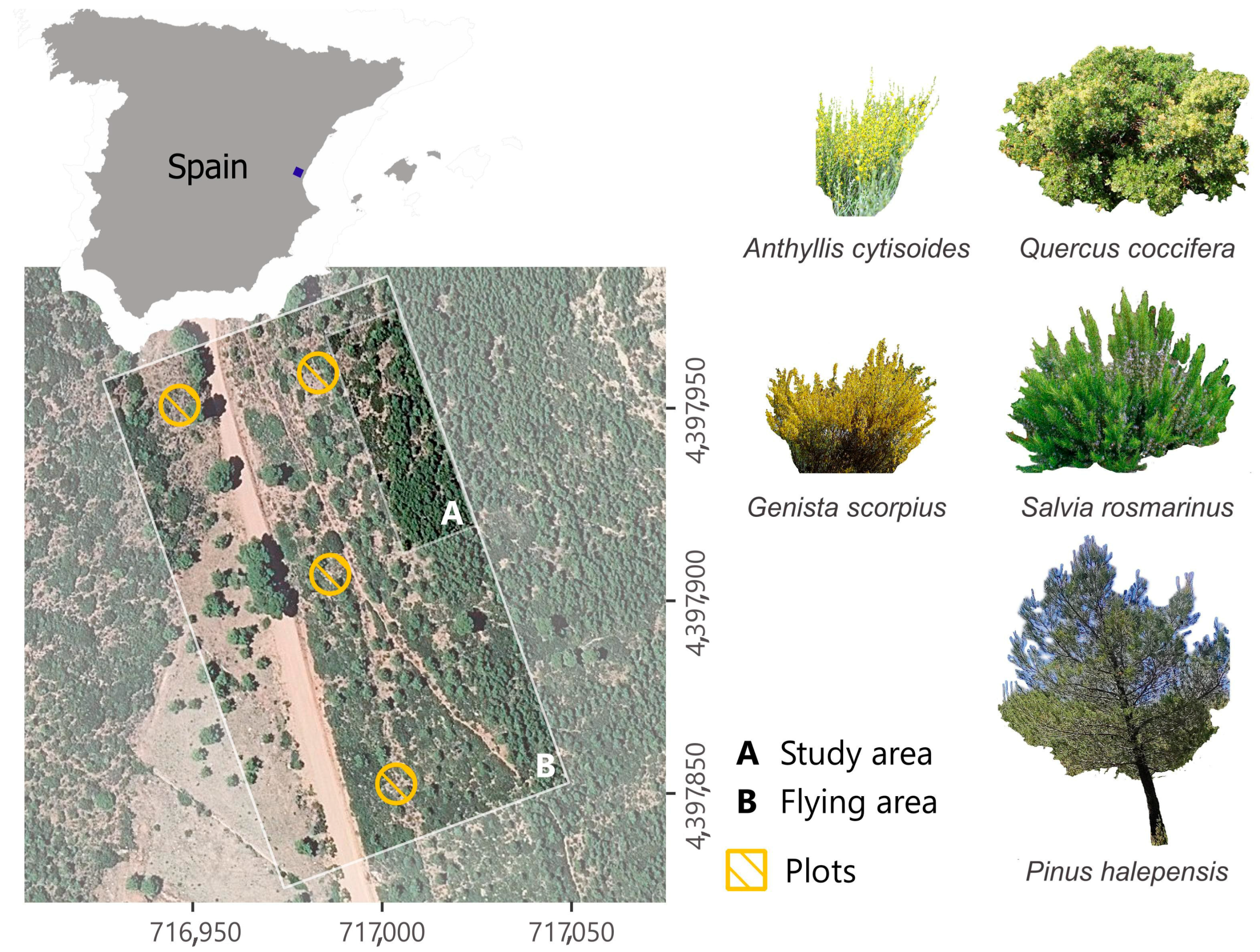
A broad field campaign was carried out in June 2022, where standard forest inventory measurements were collected in 22 circular plots with a 5 m radius: diameter at breast height (DBH) and tree height for all trees in the plot, shrub position, height, crown size, and orientation. All species were identified, and the position of plant individuals was registered using real-time kinematic GNSS equipment with a nominal horizontal accuracy of ±2 cm. The selection of plots was performed following a restricted randomization scheme [15], conditioned by diversity and representativeness of species, density of vegetation, slope, and mobile coverage for accurate GNSS geolocation. However, in this work, we are only focusing on the four plots of Figure 1 for the creation and evaluation of biomass models, and in subarea “A” for the fire simulation. Figure 1 also shows the five vegetation species available in our specific study area.

Data acquisition with UAS was carried out with a DJI Inspire 2 equipped with a DJI Zenmuse X5S camera (SZ DJI Technology Co., Shenzhen, China), obtaining images with three visible spectral bands: red, green, and blue (RGB). Two different flights were performed, one at 60 m of flying height and a camera angle of 60°, and the second at a height of 120 m and a nadiral orientation (90°), both with an overlap of 80%. A crosshatch flight pattern was followed in both cases. This combination of oblique and nadir imagery has been used to reduce shadowing, while the use of different flight heights was intended to minimize surface deformation during the photogrammetric model generation. A total of 12 ground control points were geolocated throughout the whole flying area, specifically in the center, around the edges of the flight area, and in areas of maximum slope change, for the proper geometric correction of the model.

2.2. Data Preprocessing

Based on the individual plant field measurements, the AGB of every shrub and tree was estimated by applying different allometric equations per species. Thus, for A. cytisoides, we used the allometric equation proposed by [16]; for Q. coccifera, the one proposed by [17]; for G. scorpius [18]; for S. rosmarinus [19]; and for P. halepensis [20]. These values were used as reference data for the subsequent generation of AGB models.

Point clouds were generated using SfM and Metashape image processing software (version 2.0.2, Agisoft Metashape, St. Petersburg, Russia). Based on the two-dimensional images with a high degree of overlap obtained in the field with UAS, this technique generates the point cloud by finding matching features across multiple images and using these correspondences to determine the camera’s position and orientation, and the three-dimensional structure of the scene. The point cloud was then normalized with respect to the terrain. To achieve this, the point cloud was classified into ground and vegetation points using training samples and the Class3Dp software (version 1.0) [21]. Ground-classified points were interpolated to create a surface, the digital terrain model (DTM), and the elevation of all other points was calculated with respect to the DTM, resulting in a normalized point cloud.

2.3. Species Segmentation and Point Cloud Classification

The classification of point clouds into the different tree and shrub species was performed in the following three steps: (1) a preliminary supervised point cloud classification; (2) segmentation of plant individuals; and (3) reclassification of the points to homogenize the segmented individuals. For the first step, a set of RGB spectral and geometric features, analyzing point neighborhoods, directly extracted from the point cloud and available in the free software Class3Dp (version 1.0), was computed. All metrics used are described in [22]. A total of five machine learning algorithms were evaluated using cross-validation and optimized by performing a fine-tuning of their hyperparameters. Once the best model was selected, a feature selection process based on the permutation feature importance was applied, resulting in a ranking of the most relevant features for the classification problem. Then, a forward stepwise feature selection process was applied until the learning curve was stable. The second step, point cloud segmentation, was performed using the lidR package [23] at two levels, one for trees and the other for shrubs. Finally, the third step consisted of assigning all the points belonging to a segmented individual to the most frequent class.

2.4. Species-Specific Biomass Estimation

A different biomass prediction model was built for each of the five species tested. First, an ellipse was fitted for each individual point cloud segment, retrieving the two axes, the perimeter, and the area. Then, the same features extracted from Class3Dp were computed, and a Random Forest regression was applied using the four best features selected from the feature importance permutation, in order to avoid overfitting. The five models obtained, one per species, were evaluated using 10-fold cross-validation, and applying the allometric equations to the field collected measurements per individual plant. Coefficient of determination (R²) and root mean squared error (RMSE) were used for the evaluation of regression models.

2.5. Fire Behavior Simulation and Sensitivity Analysis

Once the biomass per individual was estimated, it was divided into different voxels composing the plant. To do this, we calculated the ratio of the number of points within each voxel by the total number of points at the individual level, and without considering a minimum number of points due to the voxel size employed. These ratio values gave us an estimation of the relative number of points at the individual and voxel level. Therefore, multiplied by the predicted biomass per individual, we obtained the biomass at the individual and voxel level. Next, to estimate the bulk density at the same level, we divided the biomass values of each voxel by its volume. In scenarios where two or more individuals overlapped, the average bulk density values of the overlapping individuals were calculated for that voxel, since a sum overestimated the values for the simulation scenarios. The whole scenario of 20 m by 60 m, corresponding to area “A” in Figure 1, was built to run wildfire simulations using Fire Dynamics Simulator (FDS) software, a Computational Fluid Dynamics (CFD) model developed by the National Institute of Standards and Technology of the United States of America (NIST). The model is under continuous development and validation, and its current state of validation, which has been mostly carried out in the Northwest of the USA and at lab scale rather than field scale, can be checked in [24].

A total of 20 different simulations were run by modifying the input parameters of wind speed and fuel moisture content (FMC), with a duration of 150 s each. Thus, four wind speed values of 2.5, 5, 7.5, and 10 (m·s⁻¹), and five fuel moisture content percentages of 14%, 30%, 45%, 60%, and 75% were tested. For each scenario, the same FMC was given to each species. A sensitivity analysis was performed by interpreting three different output parameters: heat release rate (HRR), rate of spread (RoS), and burnt biomass.

3. Results and Discussion

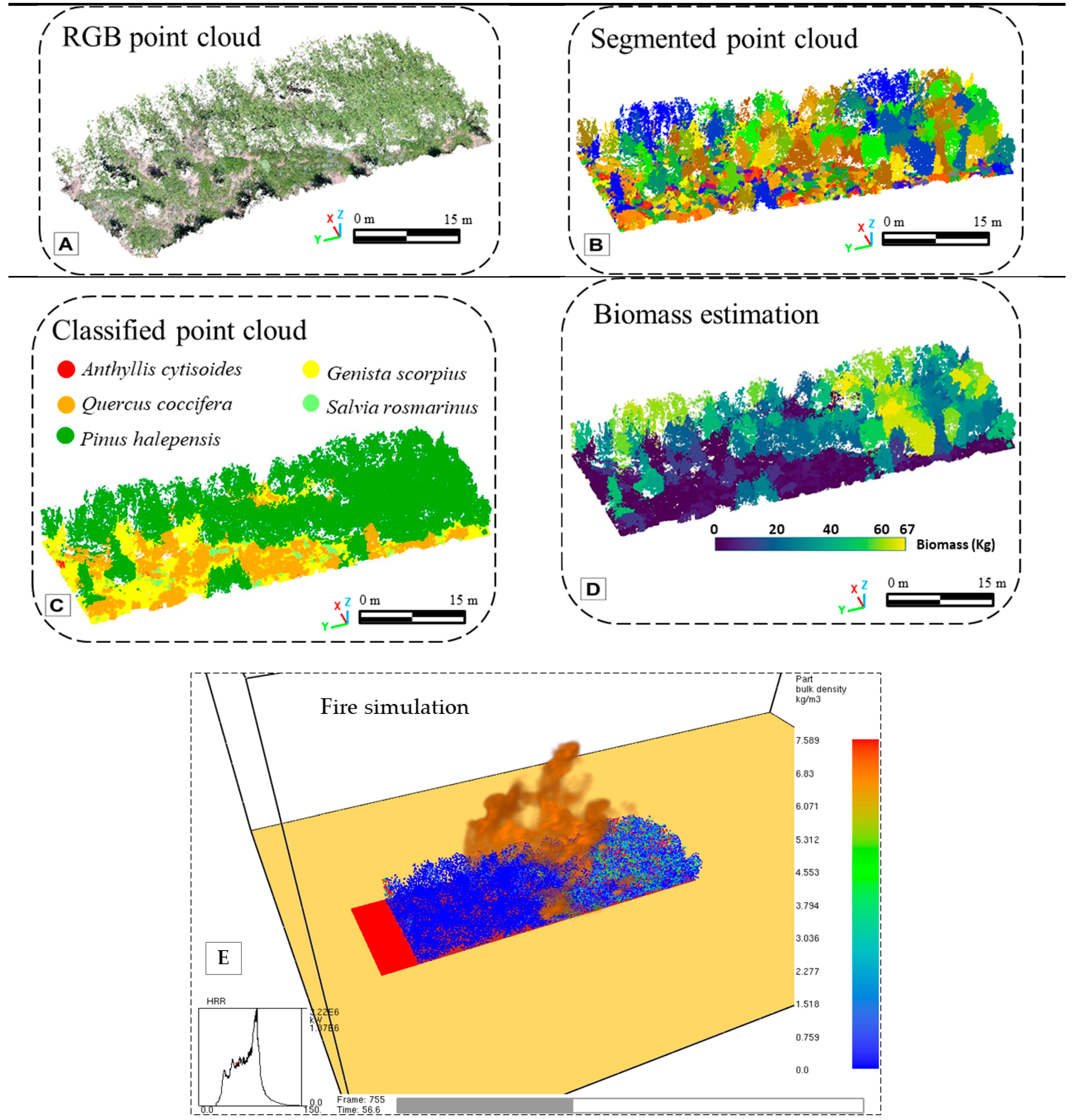
Figure 2 shows a representation of the intermediate results from the preprocessing steps generating the point cloud to the wildfire simulations.

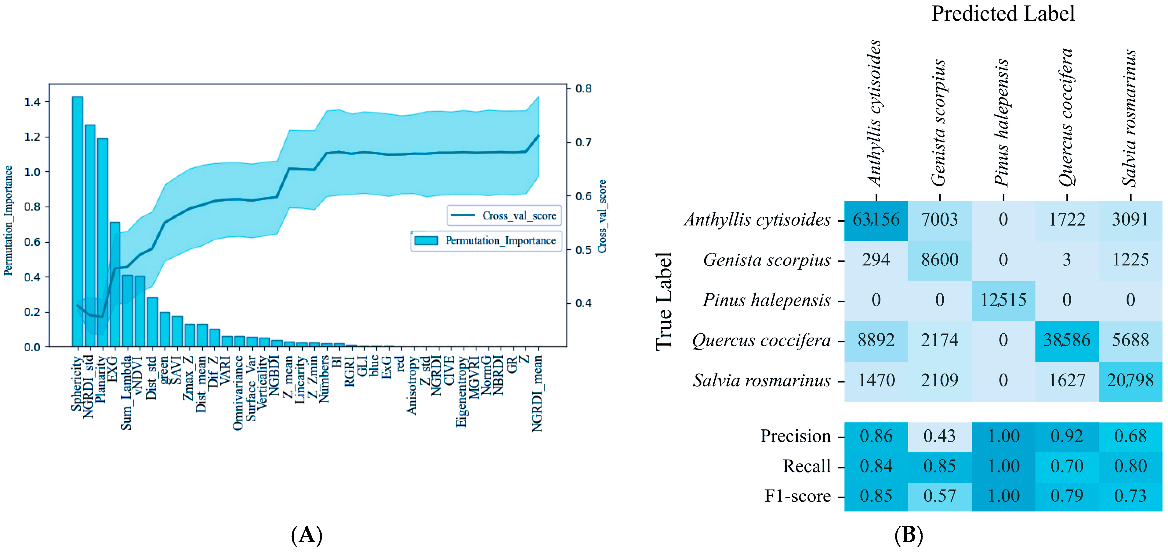
Regarding the point cloud classification results, Figure 3A shows the permutation importance of the variables used in the classification using the Random Forest algorithm. As expected, there is a combination of geometric and spectral features among the most relevant, pointing to the complementarity of both. After applying the stepwise introduction of the variables, the same figure shows the evolution of overall accuracy using cross-validation. Using only a reduced set of features, the accuracy values become stable at about 0.7 of the overall accuracy in classifying the point cloud. Figure 3B shows the error matrix and the classification indices per class. Even if the overall accuracy is 80.3%, there are important differences between species, so we can see how taller species, such as Pinus halepensis and even Quercus coccifera, are classified with much greater accuracy than smaller species, in particular Genista Scorpius, whose precision score is only 0.43 and is mainly confused with Anthyllis cytisoides. Although these results are promising, the models were trained on a limited number of species and a single-season sampling design, which precluded accounting for seasonal phenological and morphological changes.

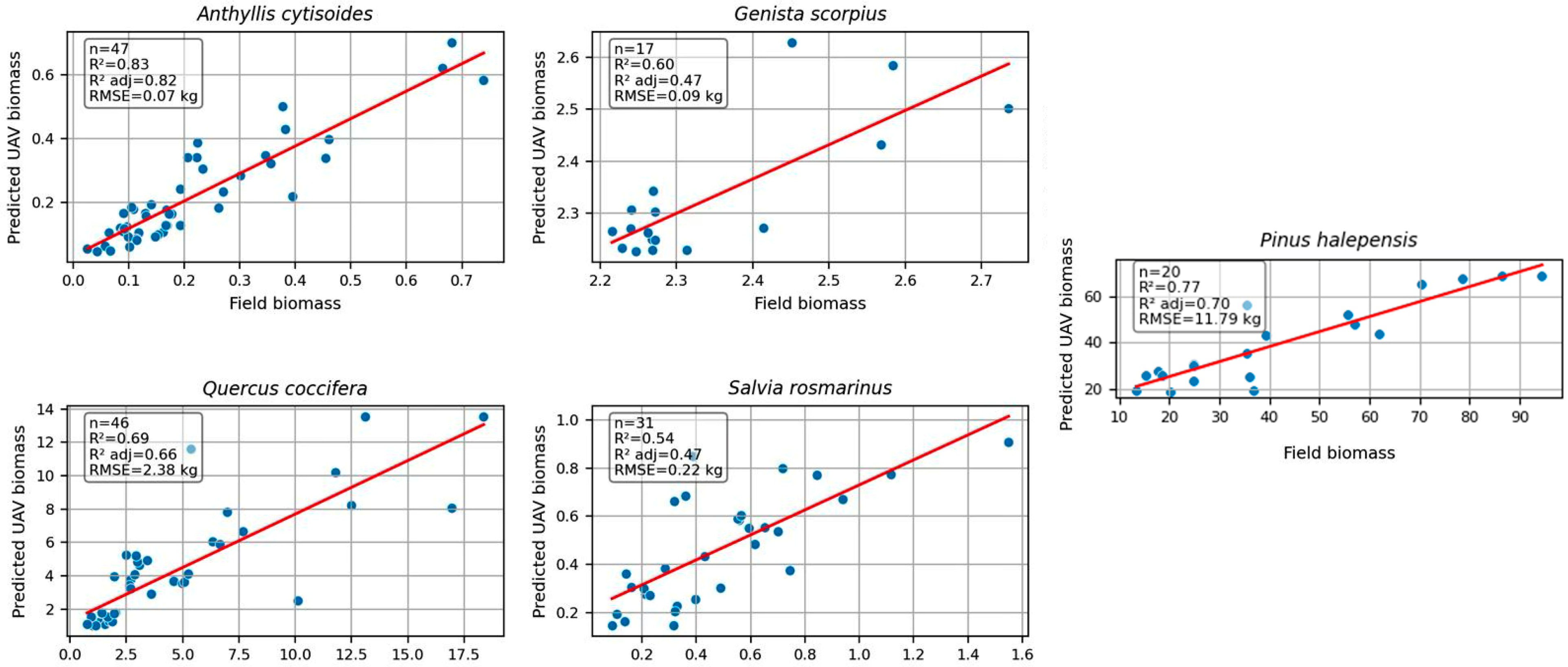
The evaluation indices and scattergrams obtained for the biomass prediction models of the five species, as compared to the reference ones based on field measurements and the allometric equations used, are shown in Figure 4. Even if the number of cases (n) available to build the models was low, particularly for G. scorpius and P. halepensis, we can see encouraging trends and results in terms of R² and RMSE, especially for A. cytisoides and P. halepensis, with R² of 0.83 (RMSE = 0.07 Kg) and 0.77 (RMSE = 11.79 Kg), respectively.

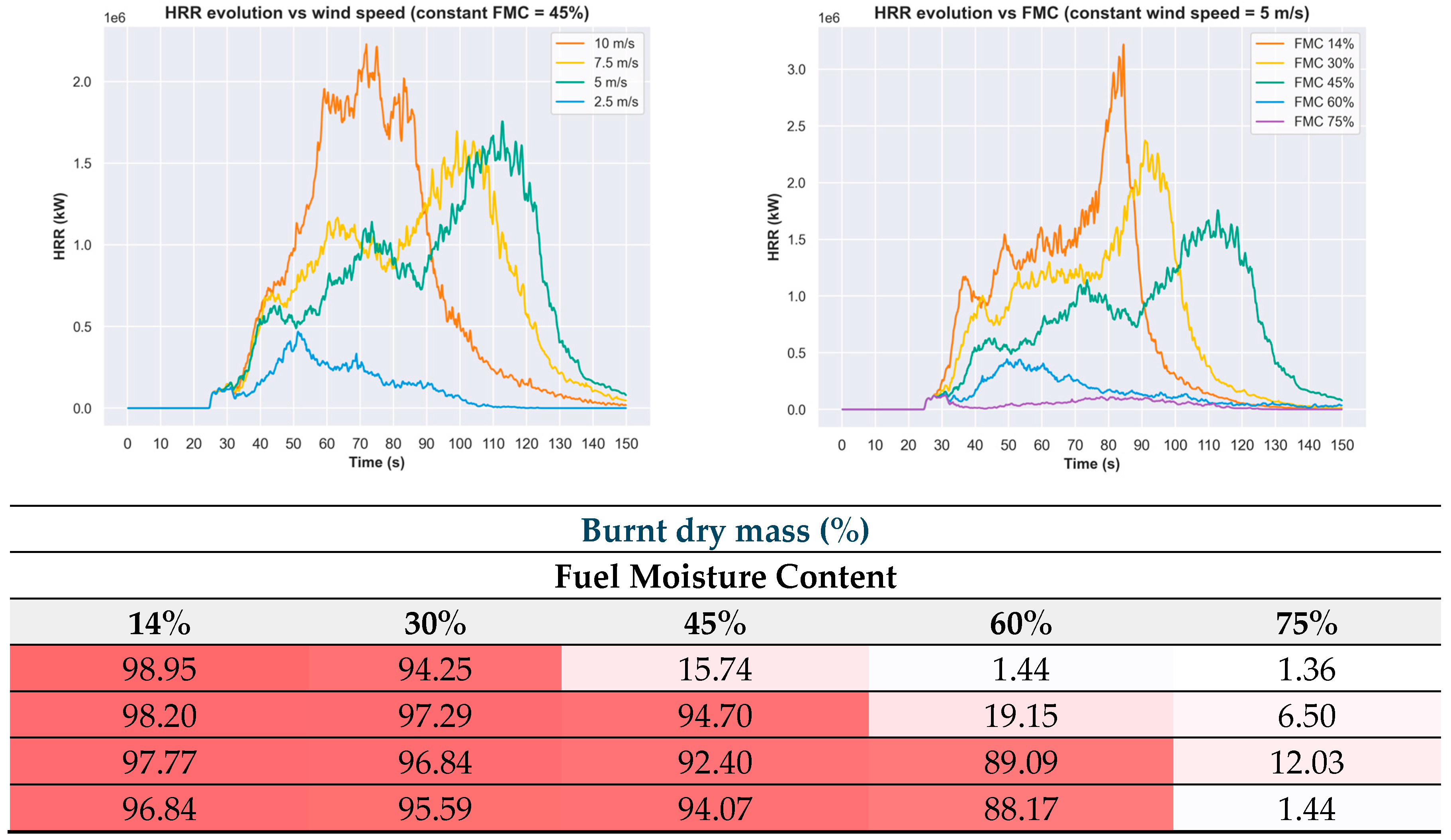
Analyzing the 20 wildfire simulations run with FDS, after converting the biomass per individual to bulk density, we obtained the evolution of fire behavior variables such as heat release rate, rate of spread, and burnt dry mass during the duration of the tests (150 s). Figure 5 shows a table with the variation in the total burned dry mass in the study area as the parameters of wind speed and fuel moisture content are modified. In most scenarios, all the biomass is practically burned, except in those where the combination of low wind speed and high fuel moisture content restricts the total burning of the fuel biomass. This information may help to define the risk assessment and prediction for real scenarios, such as the one defined by the point clouds acquired in our study area. Examining the two graphs of Figure 5, we can see how, for a constant value of FMC (i.e., 45%), only in the case of a wind speed of 2.5 m·s⁻¹, the biomass is not totally burned. However, the evolution of the HRR is faster as the wind speed increases, meaning that the RoS is also higher, which is an important parameter to consider for firefighting operations. Conversely, for a constant wind speed (i.e., 5 m·s⁻¹), FMC greater than 60% avoids the total burning of the fuel biomass, and as the FMC has lower values, the combustion is faster.

From our simulations, we identify the following actionable thresholds: fires remain patchy when wind speeds are below 2.5 m·s⁻¹ and fuel moisture exceeds 30%, whereas rapid, continuous spread is triggered above 5 m·s⁻¹ wind and moisture below 45%. These thresholds can guide ignition planning, prescribed-burn safety, and resource allocation in operational settings. Based on this methodology and results, further simulations using a variety of environmental parameters will be performed in the future.

4. Conclusions

Our preliminary research in a Mediterranean forest shows that UAS point cloud data have the potential to facilitate the use of 3D physics-based fire behavior models. Specifically, (i) multi-species classification via UAS-SfM point clouds and RGB data achieved an overall accuracy of 80.3%; (ii) individual-plant biomass estimation models reaching cross-validation R² values from 0.54 to 0.83; and (iii) sensitivity analyses on wind speed and fuel moisture content elucidated their quantitative effects on rate of spread, heat release rate, and mass loss. Biomass estimation models at the individual and species levels obtained from UAS point clouds and RGB spectral data have shown promising results, but they still require improvement. In particular, increasing the number of samples and incorporating inter-seasonal acquisitions would help capture variability in greenness and flowering. Moreover, integrating more comprehensive datasets, such as multispectral or hyperspectral imagery, would enhance both the classification of shrub species composition and the accuracy of biomass predictions.

Three-dimensional fire behavior models are useful to test the effect of forest conditions and meteorological variables, such as fuel moisture content and wind speed, on the propagation of fire. This can be used to improve wildfire prediction and risk, forest management practices, and the monitoring of fire evolution. Future work should integrate sensors with more spectral bands, as well as explore 3D canopy moisture modeling, real-time UAS deployment for fuel mapping during fire, and field-based validation in drought-stressed stands to assess robustness under extreme conditions in Mediterranean ecosystems.