Indirect Measurement of Tensile Strength of Materials by Grey Prediction Models GMC(1,n) and GM(1,n) ^†

Abstract

Grey theory is applied to forecasting, decision-making, and control as this theory is appropriate for predictive analysis. Incomplete information is a primary characteristic of the grey system, necessitating the supplementation of information to transform the relationships between various information elements from grey to white and improve the accuracy of predictive models. However, for the first-order grey prediction model with n variables, specifically the traditional GM(1,n) model, modelling values are derived using a rough approximation method. It is assumed in this method that the elements of the one-order accumulated generating series of each associated series are constant, leading to an unreasonable relationship between the forecast series and the associated series, which is fundamentally an incorrect model. The elements of a non-negative series’s one-order accumulated generating series cannot be constants; even if they are constant series, this is not true. Consequently, the traditional GM(1,n) model yields significant errors. There have been few papers addressing the errors of this model. To improve the GM(1,n) model, correct algorithms must be used by incorporating convolution algorithms or fitting system action quantities with basic functions to derive particular solutions. The modelling procedure of the grey convolution prediction model GMC(1,n) demonstrates that the traditional grey prediction model GM(1,n) is incorrect.

1. Introduction

The grey prediction model is based on the GM(1,1) model, which is currently the most widely applied. However, the GM(1,1) model provides accurate forecasts only for generalized energy systems, specifically those whose behavioural characteristics conform to exponential laws. Incomplete information is a primary characteristic of grey systems, necessitating the supplementation of information to transform the system from grey to white. The multi-series traditional grey prediction model GM(1,n) was proposed for this purpose [1,2].

Grey system theory was introduced by Deng [3]. It is particularly appropriate for predictive analysis [1]. Due to the evident exponential patterns in the new series generated through accumulation, differential equations are established for fitting. Among these, the first-order grey differential equation is the most common. For the first-order grey prediction model with n variables, namely the traditional GM(1,n) model, only relatively rough approximation methods have been proposed [1,2]. These methods assume that the elements of the one-order accumulated generating series of each associated series are constant, deriving approximate relationships between the forecast series and the associated series. However, this method is not correct. The approximation methods of the traditional GM(1,n) model are unreasonable, leading subsequent researchers to continue using them, resulting in a lower forecasting accuracy [4]. Therefore, the fundamental principle is not correct when grey systems improve forecast accuracy by introducing associated series to supplement information. “In the GM(N,H) model, the constructed model cannot be used for forecasting; it can only be used to analyze the relationships among factors” [2].

2. Grey Prediction Model

For n variables, X₁, X₂, …, X_n, which represent a total of n original series,

$${X_i}^{(0)}=\{{X_i}^{(0)}(1),{X_i}^{(0)}(2),\dots ,{X_i}^{(0)}(r)\}, i=1,2,\dots ,n,$$

(1)

Applying a first-order accumulated generating operation (abbreviated as 1-AGO) to X_i⁽⁰⁾, we obtain

$${X_i}^{(1)}=\{{X_i}^{(1)}(1),{X_i}^{(1)}(2),\dots ,{X_i}^{(1)}(r)\},i=\mathrm{1,2},\dots ,n$$

(2)

where

$${X_i}^{(1)}(k)=\sum _{j=1}^k{X_i}^{(0)}(j),i=\mathrm{1,2},\dots ,n$$

(3)

This enables the whitening form of the differential equation. The traditional grey prediction model GM(1,n) and the grey convolution prediction model GMC(1,n) are established as follows.

2.1. Traditional Grey Prediction Model GM(1,n)

The traditional GM(1,n) model is expressed as

$${\displaystyle \frac{d{X_1}^{(1)}(t)}{dt}}+b_1{X_1}^{(1)}(t)=b_2$$

(4)

Furthermore, from the definition of the derivative,

$${\displaystyle \frac{d{X_1}^{(1)}(t)}{dt}}=\underset{\Delta t\to 0}{lim}{\displaystyle \frac{{X_1}^{(1)}(t+\Delta t)-{X_1}^{(1)}(t)}{\Delta t}}$$

(5)

Setting $\Delta t$ = 1,

$${\displaystyle \frac{d{X_1}^{(1)}(t)}{dt}}={X_1}^{(1)}(t+1)-{X_1}^{(1]}(t)=X_1^{(0)}(t+1)$$

(6)

The background value of ${\displaystyle \frac{d{X_1}^{(1)}(t)}{dt}}$ is taken as the average of the values at the current time and the subsequent unit time, that is $[X_1^{(1)}(t+1)+X_1^{(1)}(t)]/2.$

For the associated series, it is directly taken as $X_i^{(1)}(t),i=\mathrm{2,3},\dots ,n.$ Let the parameter series of (4) be $[b_1,b_2,\dots ,b_n{]}^T.$

Then, the system parameters are obtained using the least squares method.

$$[b_1,b_2,\dots ,b_n{]}^T=(B^{T}B{)}^{-1}{B}^T{Y}_N$$

(7)

where

$$B=\left[\begin{array}{cc}-{\displaystyle \frac{1}{2}}({X_1}^{(1)}(1)+{X_1}^{(1)}(2)),& {X_2}^{(1)}(2),\\ -{\displaystyle \frac{1}{2}}({X_1}^{(1)}(2)+{X_1}^{(1)}(3)),& {X_2}^{(1)}(3),\\ \dots & \dots \\ -{\displaystyle \frac{1}{2}}({X_1}^{(1)}(r-1)+{X_1}^{(1)}(r)),& {X_2}^{(1)}(r),\end{array}\right.$$

(8)

and

$$Y_N=[{X_1}^{(0)}(2),{X_1}^{(0)}(3),\dots ,{X_1}^{(0)}(r){]}^T$$

(9)

Assuming that the elements of the one-order accumulated generating series of each associated series are constant, the approximate relationship for the elements of the one-order accumulated generating series of the forecast series is

$$\begin{gathered} {{\widehat{X}}_1}^{(1)}(t)=[{X_1}^{(0)}(1)-{\displaystyle \frac{1}{b_1}}\sum _{i=2}^n{b}_i{X_i}^{(1)}(t)]e^{-b_1(t-1)}+ \\ {\displaystyle \frac{1}{b_1}}\sum _{i=2}^n{b}_i{X_i}^{(1)}(t) \end{gathered}$$

(10)

By performing an inverse first-order generating operation abbreviated as 1-IAGO, the modelling values of the GM(1,n) model (before the forecast origin) and the forecast values or indirect measurements (after the forecast origin) are given by

$${\widehat{X}}_1^{(0)}(1)={\widehat{X}}_1^{(0)}(1)$$

(11)

and

$${\widehat{X}}_1^{(0)}(t)={\widehat{X}}_1^{(1)}(t)-{\widehat{X}}_1^{(1)}(t-1),t=\mathrm{2,3},\dots n$$

(12)

2.2. Grey Convolution Prediction Model GMC(1,n)

The GMC(1,n) model is derived from the traditional GM(1,n) model through the following improvements.

The differential equation of the GM(1,n) model is augmented with a grey control parameter u equivalent to that of the GM(1,1) model. Thus, if the associated series are removed, GM(1,n) completely degenerates into GM(1,1) (making GM(1,1) a special case of GM(1,n)). If the GM(1,1) model of the forecast series is well fitted, using the simple least squares method for system parameter determination leads to a relative reduction in the coefficients of the associated series in GM(1,n).

When determining system parameters, both the associated series part and the background value of ${\displaystyle \frac{d{X_1}^{(1)}(t)}{dt}},$ X₁⁽¹⁾(t), are taken as the average of the values at the current time and the subsequent unit time, preventing issues with time lag between the series. After obtaining the system parameters, the unit impulse response function h(t) is calculated, followed by forecasting for the associated series. Then, the system action quantity series f(t) is derived from the associated series and parameter series. The modelling values and forecast values are obtained through the convolution integral of h(t) and f(t) The improved model GMC(1,n) can be established as follows.

From (2), the whitening form of the differential equation for the GMC(1,n) model is established as (13).

$$\begin{gathered} {\displaystyle \frac{d{X_1}^{(1)}(t)}{dt}}+b_1{X_1}^{(1)}(t)=b_2{X_2}^{(1)}(t) \\ +b_3{X_3}^{(1)}(t)+\dots +b_n{X_n}^{(1)}(t)+u \end{gathered}$$

(13)

This is a first-order grey differential equation model with n variables, denoted as GMC(1,n) [5]. Here, X₁⁽⁰⁾ is the forecast series; X_i⁽⁰⁾, i = 2, 3, …n represents the associated series; b₁ and u are the grey development coefficient and grey control parameter of GMC(1,n), respectively; and b_i, i = 2, 3, …n represents the associated coefficients of GMC(1,n). Then, from the definition of the derivative,

$${\displaystyle \frac{d{X_1}^{(1)}(t)}{dt}}=\underset{\Delta t\to 0}{lim}{\displaystyle \frac{{X_1}^{(1)}(t+\Delta t)-{X_1}^{(1)}(t)}{\Delta t}}$$

(14)

Taking $\Delta t$ = 1,

$${\displaystyle \frac{d{X_1}^{(1)}(t)}{dt}}={X_1}^{(1)}(t+1)-{X_1}^{(1]}(t)=X_1^{(0)}(t+1)$$

(15)

The background value $X_1^{(1)}(t)$ of ${\displaystyle \frac{d{X_1}^{(1)}(t)}{dt}}$ is usually taken as $[X_1^{(1)}(t+1)+X_1^{(1)}(t)]/2.$ Let the parameter series of (13) be $[b_1,b_2,\dots ,b_n,u{]}^T$. Then, the parameters can be obtained using the least squares method as follows.

$$[b_1,b_2,\dots ,b_n,u{]}^T=(B^{T}B{)}^{-1}{B}^T{Y}_N,$$

(16)

where

$$B=\left[\begin{array}{cccccc}-{\displaystyle \frac{1}{2}}({X_1}^{(1)}(1)+{X_1}^{(1)}(2)),& {\displaystyle \frac{1}{2}}({X_2}^{(1)}(1)+{X_2}^{(1)}(2)),& {\displaystyle \frac{1}{2}}({X_3}^{(1)}(1)+{X_3}^{(1)}(2))& \dots ,& {\displaystyle \frac{1}{2}}({X_n}^{(1)}(1)+{X_n}^{(1)}(2)),& 1.0\\ -{\displaystyle \frac{1}{2}}({X_1}^{(1)}(2)+{X_1}^{(1)}(3)),& {\displaystyle \frac{1}{2}}({X_2}^{(1)}(2)+{X_2}^{(1)}(3)),& {\displaystyle \frac{1}{2}}({X_3}^{(1)}(2)+{X_3}^{(1)}(3))& \dots ,& {\displaystyle \frac{1}{2}}({X_n}^{(1)}(2)+{X_n}^{(1)}(3)),& 1.0\\ \dots & \dots & & & \dots & \\ -{\displaystyle \frac{1}{2}}({X_1}^{(1)}(r-1)+{X_1}^{(1)}(r)),& {\displaystyle \frac{1}{2}}({X_2}^{(1)}(r-1)+{X_2}^{(1)}(r)),& {\displaystyle \frac{1}{2}}({X_3}^{(1)}(r-1)+{X_3}^{(1)}(r))& \dots ,& {\displaystyle \frac{1}{2}}({X_n}^{(1)}(r-1)+{X_n}^{(1)}(r)),& 1.0\end{array}\right]$$

(17)

and

$$Y_N=[{X_1}^{(0)}(2),{X_1}^{(0)}(3),\dots ,{X_1}^{(0)}(r){]}^T$$

(18)

Substituting (16) into (13) allows us to solve for the fitted grey differential equation. The procedure for solving (13) is as follows.

Assume there is an input function x(t) that, after passing through a system, produces an output function y(t). When x(t) = δ(t), where δ(t) is a unit impulse function, the resulting y(t) is referred to as the unit impulse response function h(t). If the system is linear, then when x(t) = x₀δ(t), it follows that y(t) = x₀h(t). If the input function x_τδ(t) has a delay τ, then the output function must be x_τh(t − τ), where x_τ is the magnitude of the input function. When the input function x(t) is a combination of continuous signals, the output function y(t) is the integral of the output functions caused by all individual signals.

$$y(t)={\int }_0^{t}x(\tau )h(t-\tau )d\tau$$

(19)

Using the Laplace transform [6] to determine the unit impulse response function h(t) from (13), the procedure is as follows. The unit impulse response function can be obtained from (13) by

$${\displaystyle \frac{d{X_1}^{(1)}(t)}{dt}}+b_1{X_1}^{(1)}(t)=\delta (t)$$

(20)

where δ(t) is the unit impulse function. Taking the Laplace transform of both sides of (20), when ${X_1}^{(1)}(1)=0$,

$$s{{\stackrel{-}{X}}_1}^{(1)}(s)+b_1{{\stackrel{-}{X}}_1}^{(1)}(s)=1$$

(21)

or

$${{\stackrel{-}{X}}_1}^{(1)}(s)={\displaystyle \frac{1}{s+b_1}}$$

(22)

Taking the inverse transform,

$${X_1}^{(1)}(t)=e^{-b_{1}t}$$

(23)

This is the unit impulse response function h(t). However, in grey models, the series indices typically start counting from t = 1, so

$${X_1}^{(1)}(t)=e^{-b_1(t-1)}$$

(24)

This is the unit impulse response function h(t). Therefore, if we let the right side of (13) be f(t), then

$${\displaystyle \frac{d{X_1}^{(1)}(t)}{dt}}+b_1{X_1}^{(1)}(t)=f(t)$$

(25)

Once the parameters of (13) are determined, the discrete data for the system action quantity f(t) can be obtained. The modelling values are derived from the convolution integral of f(t) and h(t), leading to the solution

$${{\widehat{X}}_1}^{(1)}(t)={X_1}^{(1)}(1)e^{-b_1(t-1)}+{{\int }_1^{t}e}^{-b_1[t-1-(\tau -1)]}f(\tau )d\tau$$

(26a)

f(t) also starts counting from t = 1, so the exponent in the integrand includes (τ − 1). By applying the trapezoidal rule,

$$\begin{gathered} {{\widehat{X}}_1}^{(1)}(t)\cong {X_1}^{(1)}(1)e^{-b_1(t-1)}+u(t-2)\times \{0.5\times e^{-b_1(t-1)}f(1)+ \\ \sum _2^{t-1}[e^{-b_1(t-\tau )}f(\tau )]+0.5\times f(t)\} \end{gathered}$$

(26b)

where u(t) is the unit step function. By applying 1-IAGO to (26b), the modelling values of the GMC(1,n) model (before the forecast origin) are obtained, and the forecast values or indirect measurement values (after the forecast origin) are calculated as

$${\widehat{X}}^{(0)}(1)={\widehat{X}}^{(1)}(1)$$

(27)

and

$${\widehat{X}}^{(0)}(t)={\widehat{X}}^{(1)}(t)-{\widehat{X}}^{(1)}(t-1),t=\mathrm{2,3},\dots n$$

(28)

Since the GMC(1,n) modelling values are based on the linear grey differential Equation (4) or (13), the derived algorithm for the individual action quantities of the system, which follows the principle of superposition, represents a correct solution. If we derive the system action quantity $\sum _{i=2}^n{b}_i{X_i}^{(1)}(t)$ by substituting the parameters obtained from the traditional GM(1,n) model back into Equation (4), we find that it corresponds to $f(\tau )$ in (26a). In other words, regardless of whether the parameter estimation methods of the traditional GM(1,n) model are correct, the appropriate calculation for the modelling values of the one-order accumulated generating series must be

$${{\widehat{X}}_1}^{\left(1\right)}\left(t\right)={X_1}^{\left(1\right)}\left(1\right)e^{-b_1\left(t-1\right)}+{{\int }_1^{t}e}^{-b_1[t-1-(\tau -1)]}\sum _{i=2}^n{b}_i{X_i}^{(1)}(\tau )d\tau$$

(29)

If $\sum _{i=2}^n{b}_i{X_i}^{(1)}(\tau )$ is incorrectly treated in (29) (which $\tau$ is a dummy variable) as a constant, then

$${{\widehat{X}}_1}^{\left(1\right)}\left(t\right)={X_1}^{\left(1\right)}\left(1\right)e^{-b_1\left(t-1\right)}+\sum _{i=2}^n{b}_i{X_i}^{(1)}(t){{\int }_1^{t}e}^{-b_1(t-\tau )}d\tau$$

(30)

where

$${{\int }_1^{t}e}^{-b_1(t-\tau )}d\tau ={\displaystyle \frac{1}{b_1}}{\left.e^{-b_1(t-\tau )}\right|}_{\tau =1}^{\tau =t}={\displaystyle \frac{1}{b_1}}(1-e^{-b_1(t-1)})$$

(31)

Substituting (31) into (30) yields

$$\begin{gathered} {{\widehat{X}}_1}^{(1)}(t)={X_1}^{(1)}(1)e^{-b_1(t-1)}+\sum _{i=2}^n{b}_i{X_i}^{(1)}(t)\times [{\displaystyle \frac{1}{b_1}}(1-e^{-b_1(t-1)})] \\ =\left[{X_1}^{\left(0\right)}\left(1\right)-{\displaystyle \frac{1}{b_1}}\sum _{i=2}^n{b}_i{X_i}^{\left(1\right)}\left(t\right)\right]e^{-b_1\left(t-1\right)}+ \\ {\displaystyle \frac{1}{b_1}}{\sum }_{i=2}^n{b}_i{X_i}^{(1)}(t) \end{gathered}$$

(32)

This exactly corresponds to the modelling values of the one-order accumulated generating series of the traditional grey prediction model GM(1,n), as shown by the algorithm in (10). This demonstrates that the traditional grey prediction model GM(1,n) is indeed incorrect.

3. Application Example

The Brinell hardness of a certain material is an example of the associated series, modelling using both the traditional grey prediction model GM(1,n) and the GMC(1,n) model. The indirect measurements correspond to the tensile strength at higher temperatures to illustrate the accuracy of the traditional grey prediction model GM(1,n). We consider the data from

Table 1. Experimental data of Brinell hardness and tensile strength of heat-treated steel C1040: temperatures ranging from 400 °F to 1300 °F.

i (Temperature)	$\mathbf{Tensile} \mathbf{Strength} (\mathbf{MPa}) {{\mathit{X}}_1}^{(0)}(\mathit{i})$	$\mathbf{Brinell} \mathbf{Hardness} (\mathbf{HBW}) {{\mathit{X}}_2}^{(0)}(\mathit{i})$
1 (400 °F)	897	514
2 (500 °F)	897	495
3 (600 °F)	890	444
4 (700 °F)	876	401
5 (800 °F)	848	352
6 (900 °F)	814	293
7 (1000 °F)	779	269
8 (1100 °F)	738	235
9 (1200 °F)	669	201
10 (1300 °F)	600	187

,

Table 2. This table presents 1-AGO experimental data and modelling values ${\widehat{X}}_1^{(1)}(i), i=1, 2, \dots , 10$ from the traditional grey prediction model (33) for heat-treated steel C1040: temperatures ranging from 400 °F to 1300 °F.

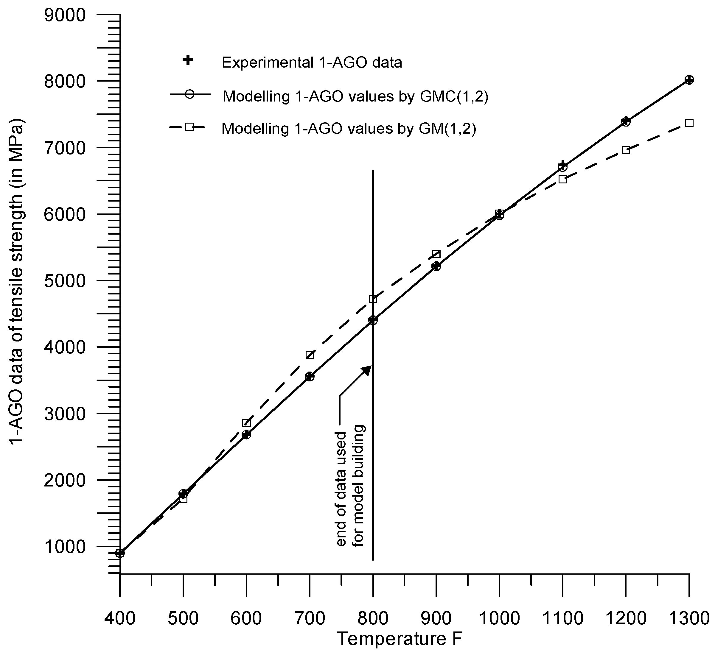
i (Temperature)	$\mathbf{Actual} 1-\mathbf{AGO} \mathbf{Data} {\mathit{X}}_1^{(1)}(\mathit{i})$ (Mpa)	$1-\mathbf{AGO} \mathbf{Data} {\widehat{\mathit{X}}}_1^{(1)}(\mathit{i})$ (Mpa) by GM(1,2)	Error Percentage
1 (400 °F)	897	897	0.00%
2 (500 °F)	1794	1718.818	−4.19%
3 (600 °F)	2684	2855.437	6.39%
4 (700 °F)	3560	3876.406	8.89%
5 (800 °F)	4408	4725.202	7.20%
6 (900 °F)	5222	5402.259	3.45%
7 (1000 °F)	6001	6004.459	0.06%
8 (1100 °F)	6739	6522.629	−3.21%
9 (1200 °F)	7408	6962.540	−6.01%
10 (1300 °F)	8008	7370.211	−7.96%

,

Table 3. Experimental data and modelling values ${\widehat{X}}_1^{(0)}(i), i=1, 2, \dots , 10$ from the traditional grey prediction model (33) for heat-treated steel C1040: temperatures ranging from 400 °F to 1300 °F.

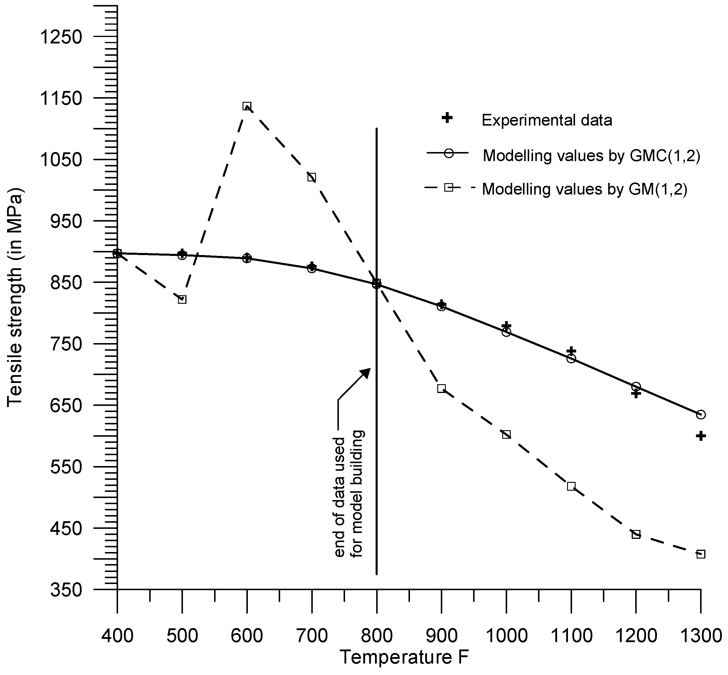
i (Temperature)	${{\mathit{X}}_1}^{(0)}(\mathit{i})$ (MPa)	${{\widehat{\mathit{X}}}_1}^{(0)}(\mathit{i})$ (MPa)	Error Percentage
1 (400 °F)	897	897	0.00%
2 (500 °F)	897	821.817	−8.38%
3 (600 °F)	890	1136.620	27.71%
4 (700 °F)	876	1020.969	16.55%
5 (800 °F)	848	848.796	0.09%
6 (900 °F)	814	677.057	−16.82%
7 (1000 °F)	779	602.201	−22.70%
8 (1100 °F)	738	518.170	−29.79%
9 (1200 °F)	669	439.911	−34.24%
10 (1300 °F)	600	407.670	−32.06%

,

Table 4. This table presents 1-AGO experimental data and modelling values ${\widehat{X}}_1^{(1)}(i), i=1, 2, \dots , 10$ from the grey convolution prediction model (34) for heat-treated steel C1040: temperatures ranging from 400 °F to 1300 °F.

i (Temperature)	$$\begin{gathered} \mathbf{Actual} \\ 1-\mathbf{AGO} \mathbf{Data} {\mathit{X}}_1^{(1)}(\mathit{i}) \end{gathered}$$ (Mpa)	$1-\mathbf{AGO} \mathbf{Data} {\widehat{\mathit{X}}}_1^{(1)}(\mathit{i})$ (Mpa) by GMC(1,2)	Error Percentage
1 (400 °F)	897	897	0.00%
2 (500 °F)	1794	1791.082	−0.16%
3 (600 °F)	2684	2680.052	−0.15%
4 (700 °F)	3560	3552.624	−0.21%
5 (800 °F)	4408	4399.342	−0.20%
6 (900 °F)	5222	5210.033	−0.23%
7 (1000 °F)	6001	5979.135	−0.36%
8 (1100 °F)	6739	6705.057	−0.50%
9 (1200 °F)	7408	7385.154	−0.31%
10 (1300 °F)	8008	8019.705	0.15%

and

Table 5. Experimental data and modelling values ${\widehat{X}}_1^{(0)}(i), i=1, 2, \dots , 10$ from the grey convolution prediction model (34) for heat-treated steel C1040: temperatures ranging from 400 °F to 1300 °F.

i (Temperature)	${{\mathit{X}}_1}^{(0)}(\mathit{i})$ (MPa)	${{\widehat{\mathit{X}}}_1}^{(0)}(\mathit{i})$ (MPa)	Error Percentage
1(400 °F)	897	897	0.00%
2(500 °F)	897	894.082	−0.33%
3(600 °F)	890	888.971	−0.12%
4(700 °F)	876	872.572	−0.39%
5(800 °F)	848	846.719	−0.15%
6(900 °F)	814	810.690	−0.41%
7(1000 °F)	779	769.102	−1.27%
8(1100 °F)	738	752.922	−1.64%
9(1200 °F)	669	680.097	1.66%
10(1300 °F)	600	634.551	5.76%

in Samuel’s book [7], which includes the actual measured values of the Brinell hardness and tensile strength of heat-treated steel C1040 (fine-grained) at temperatures ranging from 400 to 1300 °F. The material is annealed at 1450 °F, normalized at 1650 °F, and quenched in water at 1550 °F. There are 10 sets of actual measurements, as listed in Table 1. The first five sets are used for modelling, while the tensile strength data from the 6th to the 10th sets are reserved for comparison with the indirect measurement values.

Using the Brinell hardness (${X_2}^{(0)}$) as the associated series and tensile strength (${X_1}^{(0)}$) as the forecast series, the first five data points before the forecast origin (r = 5) are modelled using both the traditional grey prediction model GM(1,2) and the GMC(1,2) model to perform indirect measurements of tensile strength as follows.

3.1. Indirect Measurement Using the Traditional Grey Prediction Model GM(1,2)

Based on the first five data points from Table 1, the traditional grey prediction model GM(1,2) is established using (1)–(9).

$${\displaystyle \frac{d{X_1}^{(1)}(t)}{dt}}+1.2635{X_1}^{(1)}(t)=3.1880{X_2}^{(1)}(t)$$

(33)

Assuming the Brinell hardness data from the 6th to 10th sets $X_2^{(0)}(i),i=\mathrm{6,7},\dots ,10$ in Table 1 are measured, the values $X_2^{(1)}(i),i=\mathrm{1,2},\dots ,10$ in (33) are known. By using (10), the 1-AGO modelling values ${\widehat{X}}_1^{(1)}(i),i=\mathrm{1,2},\dots ,10$ of the traditional grey prediction model (33) are calculated, as shown in Table 2 and illustrated in Figure 1. Using (11) and (12), the modelling values ${\widehat{X}}_1^{(0)}(i),i=\mathrm{1,2},\dots ,5$ of the traditional grey prediction model (33) (before the forecast origin) and the indirect measurement values ${\widehat{X}}_1^{(0)}(i),i=\mathrm{6,7},\dots ,10$ (after the forecast origin) are obtained, as listed in Table 3 and depicted in Figure 2.

3.2. Indirect Measurement Using the Grey Prediction Model GMC(1,2)

Using the first five data points from Table 1, we can establish the grey prediction model GMC(1,2) by utilizing Equations (1)–(3) and (13)–(18) as follows

$${\displaystyle \frac{d{X_1}^{(1)}(t)}{dt}}+0.3098{X_1}^{(1)}(t)=0.6782{X_2}^{(1)}(t)+1121.09$$

(34)

Assuming the Brinell hardness data from the 6th to the 10th sets $X_2^{(0)}(i),i=\mathrm{6,7},\dots ,10$ in Table 1 are measured, the values $X_2^{(1)}(i),i=\mathrm{1,2},\dots ,10$ in (34) are known. By utilizing (19) to (26b), we can calculate the 1-AGO modelling values ${\widehat{X}}_1^{(1)}(i),i=\mathrm{1,2},\dots ,10$ of the grey convolution prediction model (34), as shown in Table 4 and illustrated in Figure 1. Further, using (27) and (28), the modelling values ${\widehat{X}}_1^{(0)}(i),i=\mathrm{1,2},\dots ,5$ of the grey convolution prediction model (34) (before the forecast origin) and the indirect measurement values ${\widehat{X}}_1^{(0)}(i),i=\mathrm{6,7},\dots ,10$ (after the forecast origin) are obtained, as listed in Table 5 and depicted in Figure 2.

4. Conclusions

Incomplete information is a primary characteristic of grey systems, necessitating the supplementation of information to transform relationships from grey to white. However, the traditional grey prediction model GM(1,n) is flawed. Among the various improved models of GM(1,n), those incorporating convolution algorithms or fitting system response quantities through basic function fitting to further derive particular solutions are valid algorithms. Figure 1 and Figure 2 and Table 2, Table 3, Table 4 and Table 5 demonstrate that the grey convolution prediction model GMC(1,2) can indeed adequately supplement information and achieve high accuracy in indirect measurement or prediction, whereas the traditional grey prediction model GM(1,n) cannot.

References

- Deng, J.L. The Elementary Method of Grey System; Huazhong University of Science and Technology Press: Wuhan, China, 1987. (In Chinese) [Google Scholar]
- Hu, L. Grey System Theory and Its Application; Science and Technological Reference Press: Beijing, China, 1992. (In Chinese) [Google Scholar]
- Deng, J.L. Control problems of grey systems. Syst. Control Lett. 1982, 1, 288–294. [Google Scholar]
- Wang, Y.; Zhang, G.; Moon, K.S.; Sutherland, J.W. Compensation for the thermal error of a multi-axis machining center. J. Mater. Process. Technol. 1998, 75, 45–53. [Google Scholar] [CrossRef]
- Tien, T.L. The indirect measurement of tensile strength of material by the grey prediction model GMC(1,n). Meas. Sci. Technol. 2005, 16, 1322–1328. [Google Scholar] [CrossRef]
- Erwin, K. Advanced Engineering Mathematics; John Wiley & Sons Inc.: Hoboken, NJ, USA, 1999. [Google Scholar]
- Samuel, L.H. Metal Data; Reinhold Publishing Corporation: New York, NY, USA, 1952. [Google Scholar]