1. Introduction
With the maturity of large-size display technology for cost reductions and the expansion of network communication bandwidth, high-resolution images such as 4 K and 8 K have become increasingly popular. Before compression, the size of high-quality images reaches several hundred megabytes. Therefore, lossless compression has become important.
Lossless image compression is conducted in the prediction and entropy encoding parts. The prediction part, however, is not limited to lossless usage. Prediction is applied to intra-frames in video coding such as high-efficiency video coding (HVEC) [
1]. The main purpose of prediction is to reduce the spatial redundancy of input images. Residues, the differences between the real pixel value and predicted value, have a small interval that originates from 0 if the predictor is precise enough. According to information theory [
2], the more the residue is centralized, the lower the entropy.
Lossless JPEG (JPEG-LS) with the median edge detector (MED) as its predictor [
3] was renamed the LOCO-I algorithm, while context-based entropy coding was added after the prediction [
4]. The predictor is simple and requires three of the causal neighbors of
N,
W, and
NW (each representing North, West, and Northwest, respectively) and
X as the predicted value (1). It uses the following equation:
The MED is based on the fact that
X is always chosen as the median value of
A,
B, and
A + B C. Despite its simplicity, the MED has a higher accuracy than the gradient-adjusted predictor (GAP), which is used in context-based adaptive lossless image coding (CALIC) [
5]. GAP predicts values according to whether the vertical/horizontal gradients nearby exceed specific thresholds. Therefore, GAP cannot fit various inputs. Another renowned predictor is the edge-directed predictor (EDP), which predicts pixel values based on the assumption that natural images have the nth Markovian property. The predicted value is obtained by using the weighted sum of causal neighbors with the weighting vector solved using the least square (LS) method. Nonetheless, due to the heavy computational load of the covariance matrix, EDP is difficult to apply. Machine learning-based methods [
6,
7] have higher accuracy compared to traditional predictor, they face a serious challenge in hardware implementation.
There have been studies to improve the MED [
8]. However, the algorithm involves k-mean clustering, which increases time complexity compared with the original MED. We re-examined the concept of the MED and proposed three methods.
2. Proposed Methods
2.1. MED from Different View
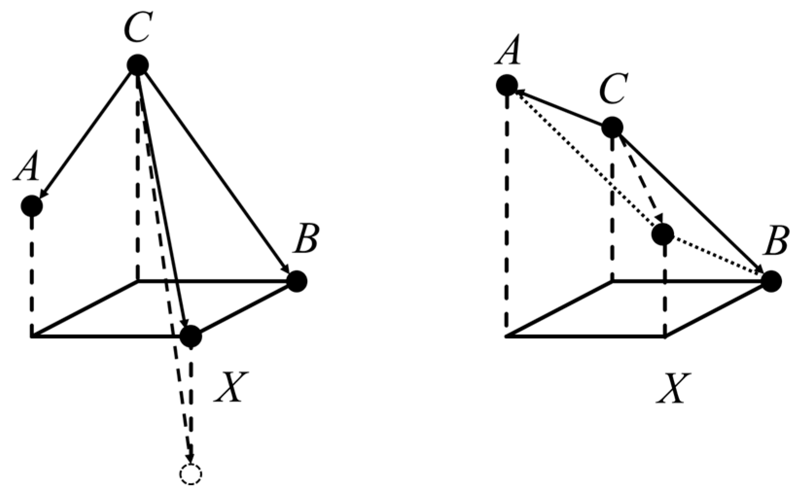
We visualized pixel values by their heights, as shown in
Figure 1. The first and second conditions in (1) were treated on the left-hand side, while the third condition was the case on the right-hand side. Considering a starting point C, we used the following equation:
To predict the value X by using a vector , the numerical value becomes A + B C, which is consistent with the third case in the MED. As for the left-hand side, we treated it as the difference of , which is bounded by a threshold and the maximum absolute value of all differences in a 2 × 2 matrix. As A + B C represented the dotted circle on the left, the actual predicted value was bounded by the vector . The MED assumed that there was no drastic change under the observed maximum difference in the 2 × 2 matrix.
2.2. MED Without Threshold and with a 3 × 3 Threshold
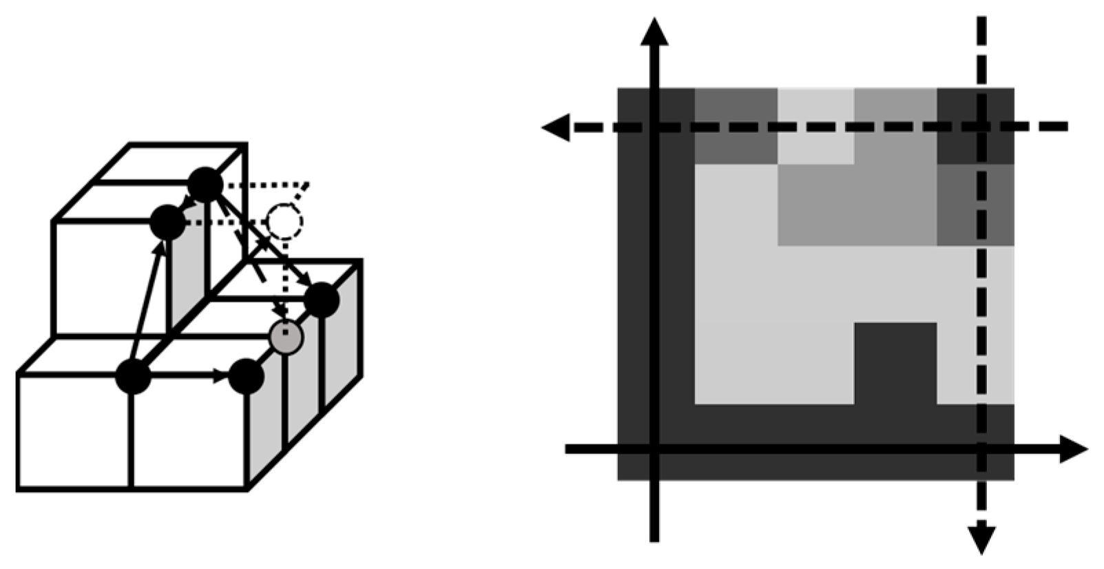
After the analysis, we explored the performance if this threshold was flexible. The first proposed method was the MED with an infinite threshold. The predicted value was A + B
C for any case. The other method was to change the original 2 × 2 matrix into a 3 × 3 matrix, as shown in
Figure 2. The threshold was set as the maximum of all differences between adjacent pixels including the diagonal direction, where 17 vectors were considered. The two methods encountered predicted values over 255 or under 0, while the input image had a bit depth of 8, and thus an additional conditional clause was added after to solve this problem.
2.3. Adaptive MED
Aside from the two methods, we considered the residue of causal parts. That is, the performance of the previous prediction became a factor to consider when predicting the current pixel. The predicted value was defined as shown in (3):
where
resA,
resB, and
resC are the residues of
A,
B, and
C in
Figure 2. If the causal residues have positive or negative signs, the predictor underestimates or overestimates in that region. Hence, the predicted value becomes the result of the original MED added with the median of the three residues.
2.4. Vertical/Horizontal Flip
Block-based compression is popular because its parallel processing shortens the time for the encoder and decoder. We introduced a vertical and horizontal flip technique to determine if the block was vertically or horizontally flipped according to the sum of squared difference (SSD). The reason why vertical/horizontal flip improves the residue is depicted on the left side of
Figure 3. Suppose the grey circle is the pixel being predicted. Based on the MED predictor, there are two different predicted values if the MED is performed by the outside and inside directions and the former one has a better predicted value.
Since the pixels at a boundary have little information for prediction, direct left or direct top are applied as predicted values. If the region is unfortunately rough at the starting point, as shown in the top-right on the right-hand side of
Figure 3, residues with large values remain. If the block is flipped vertically and horizontally, the starting point is found in the bottom left. When the boundary is smoother, the residue of the direct top and direct left is mitigated, while the predicted value in the rough region is replaced by the MED.
2.5. Residue Mapping
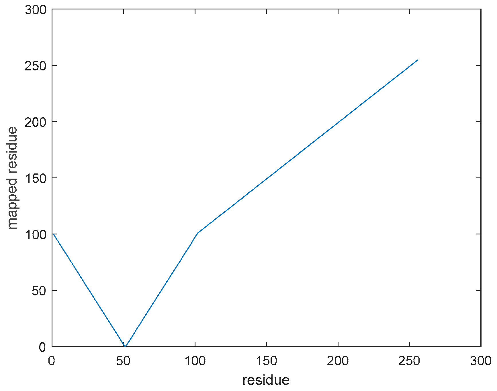
Originally, the residues were distributed on the interval [−255, 255], but little redundancy exists. That is, once the predicted value is confirmed, the residue range is located as well. For example, if the predicted value is 50, then it is impossible that the residue becomes less than −50 or more than 205. By shifting the interval [50, 205] to [100, 255], [−50, 50] can be mapped to [0, 100] by replacing their signs, as shown in
Figure 4. The mathematical form used to define an anchor point is shown in (4):
where
n is the input bit depth. By performing residue mapping, we could save the sign bit.
3. Experimental Results
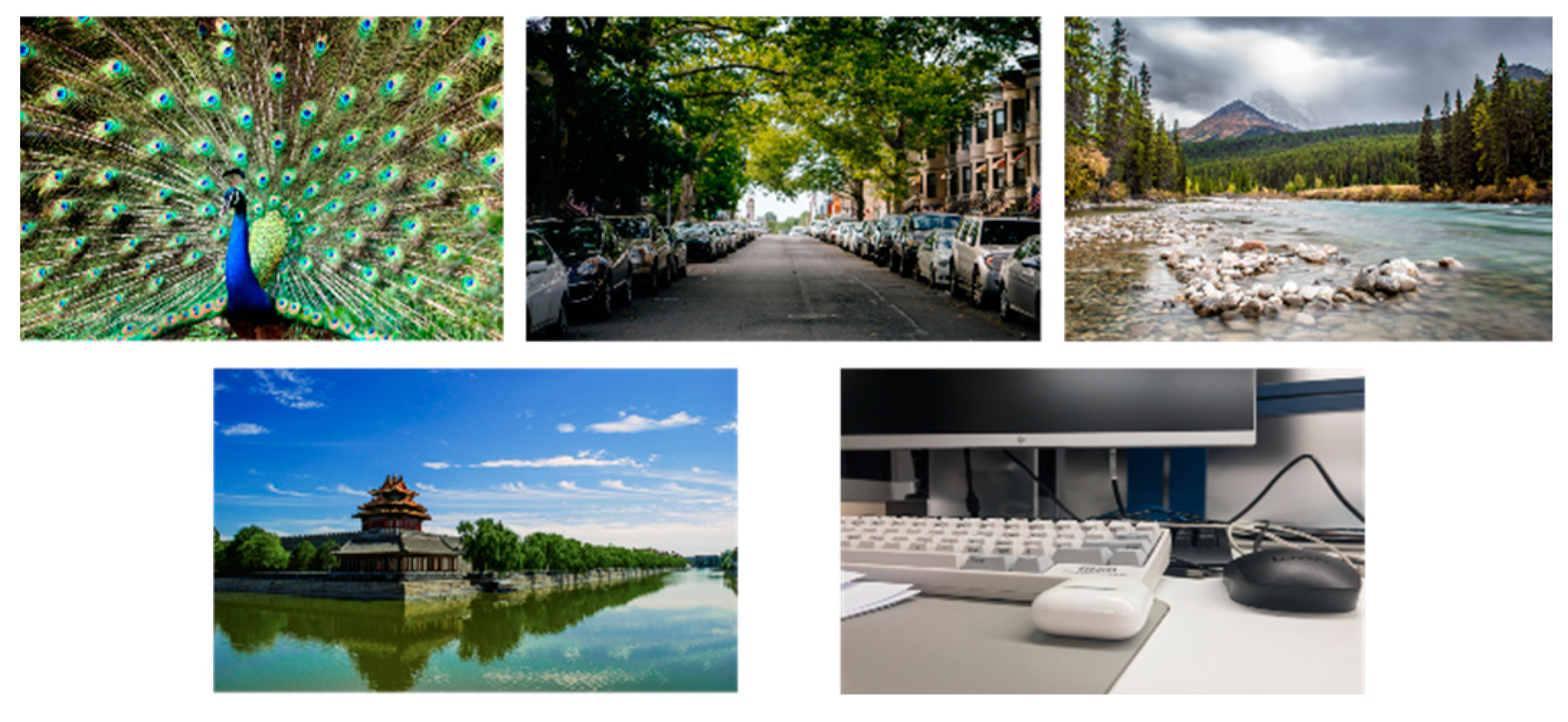
We select an experimental dataset from Ref. [
9], which contains 5 image categories. Each category has 65 images with a resolution from 4000 to 8000, on average, as shown in
Figure 5.
Table 1,
Table 2,
Table 3,
Table 4 and
Table 5 show the comparison results of entropy between the proposed method and original MED in full size, 8 × 8, 16 × 16, and 32 × 32. MED without threshold is inferior to MED in a larger size but outperforms MED in several categories when the block size is 8 × 8. By examining the dataset, we discovered that MED without threshold has an advantage when the input images are composed of complicated textures. For example, the peacock, leaves, and forest in
Figure 5 contain complicated regions, and the MED without a threshold surpasses the MED by an entropy reduction of 0.1 on average. The performance of the 3 × 3 matrix is similar to that of the MED without a threshold. It outperforms the MED in the 8 × 8 matrix and is inferior with a larger size, but unexpectedly surpasses the MED in full size.
Adaptive prediction has the lowest entropy in every category and block size. Additionally, the result of 32 × 32 is extremely close to that of the full size, which indicates that the time spent is 32/N, determined by sacrificing a few compression rates (CRs), where N is the length of the input image with the same infinite encoder and decoder.
Table 5 shows the result of the vertical flip and hybrid flip in different block sizes. The entropy is the original entropy added by the extra bits 1/(square of block size) depending on the flipped block.
If the block size is 32 × 32, the extra bpp required becomes 1/32/32 = 0.000976. The value is multiplied by 2 if the block is applied with the hybrid flip. Using only one one-direction flip is the most appropriate approach, since the trade-off between the entropy reduction and the extra bits balances the buffer to record growing residues exponentially.
4. Conclusions
We provide the other point of view on the MED to propose an improved low-complexity predictor based on the MED. While several predictors perform better than the MED only in small block sizes, the best predictor, the improved MED, outperforms the MED for all cases. In addition, a vertical/horizontal flip scheme is proposed. By spending extra bits to record the flipped block, the entropies are further reduced.
Author Contributions
Conceptualization, H.-C.H. and J.-J.D.; methodology, H.-C.H.; software, H.-C.H.; validation, H.-C.H.; formal analysis, H.-C.H. and D.-Y.L.; investigation, J.-J.D.; resources, H.-C.H.; data curation, H.-C.H.; writing—original draft preparation, H.-C.H.; writing—review and editing, D.-Y.L. and J.-J.D.; visualization, H.-C.H.; supervision, J.-J.D.; project administration, J.-J.D.; funding acquisition, J.-J.D. All authors have read and agreed to the published version of the manuscript.
Funding
This research was funded by the National Science and Technology Council, Taiwan, under the contract of NSTC 113-2221-E-002-146.
Institutional Review Board Statement
Not applicable.
Informed Consent Statement
Not applicable.
Data Availability Statement
No new data were created or analyzed in this study. Data sharing is not applicable to this article.
Conflicts of Interest
The authors declare no conflict of interest.
References
- Sze, V.; Budagavi, M.; Sullivan, G.J. High Efficiency Video Coding (HEVC); Springer: Berlin/Heidelberg, Germany, 2014. [Google Scholar]
- Shannon, C.E.; Weaver, W. The Mathematical Theory of Communication; University of Illinois Press: Champaign, IL, USA, 1963. [Google Scholar]
- Martucci, S.A. Reversible compression of HDTV images using median adaptive prediction and arithmetic coding. In Proceedings of the IEEE International Symposium on Circuits and Systems, New Orleans, LA, USA, 1–3 May 1990; pp. 1310–1313. [Google Scholar]
- Weinberger, M.J.; Seroussi, G.; Sapiro, G. The LOCO-I lossless image compression algorithm: Principles and standardization into JPEG-LS. IEEE Trans. Image Process. 2000, 9, 1309–1324. [Google Scholar] [CrossRef] [PubMed]
- Wu, X.; Memon, N. Context based, adaptive, lossless image coding. IEEE Trans. Commun. 1997, 45, 437–444. [Google Scholar] [CrossRef]
- Dumas, T.; Roumy, A.; Guillemot, C. Context-adaptive neural network-based prediction for image compression. IEEE Trans. Image Process. 2020, 29, 679–693. [Google Scholar] [CrossRef] [PubMed]
- Schiopu, I.; Munteanu, A. Deep-learning-based lossless image coding. IEEE Trans. Circ. Syst. Video Technol. 2020, 30, 1829–1842. [Google Scholar] [CrossRef]
- Amin, M.S.; Jabeen, S.; Wang, C.; Khan, H.A.; Jabbar, A. Improved median edge detection (iMED) for lossless image compression. Image Anal. Stereol. 2023, 42, 25–35. [Google Scholar] [CrossRef]
- Liu, J.; Liu, D.; Yang, W.; Xia, S.; Zhang, X.; Dai, Y. A comprehensive benchmark for single image compression artifact reduction. IEEE Trans. Image Process 2020, 29, 7845–7860. [Google Scholar] [CrossRef]
| Disclaimer/Publisher’s Note: The statements, opinions and data contained in all publications are solely those of the individual author(s) and contributor(s) and not of MDPI and/or the editor(s). MDPI and/or the editor(s) disclaim responsibility for any injury to people or property resulting from any ideas, methods, instructions or products referred to in the content. |
© 2025 by the authors. Licensee MDPI, Basel, Switzerland. This article is an open access article distributed under the terms and conditions of the Creative Commons Attribution (CC BY) license (https://creativecommons.org/licenses/by/4.0/).


