Applying a Parameterized Quantum Circuit to Anomaly Detection ^†

Abstract

In this study, a parameterized quantum circuit (PQC) is applied for anomaly detection, a crucial process to identify unusual patterns or outliers in data. PQC is a quantum circuit with trainable parameters linked to quantum gates, which are iteratively optimized by classical optimizers to ensure that the circuit’s output fulfills its objectives. This is analogous to the way of using trainable parameters, such as weights adjusted in classical machine learning and neural network models. We used the amplitude−embedding mechanism with classical data into quantum states of qubits. These states are fed into PQC, which contains strongly entangled layers, and the circuit is trained to determine whether an anomaly exists. As anomaly detection datasets are often imbalanced, resampling techniques, such as random oversampling, the synthetic minority oversampling technique (SMOTE), random undersampling, and Tomek-Link undersampling, are applied to reduce the imbalance. The proposed PQC and various resampling techniques were compared using the public Musk dataset for anomaly detection. Their combination was also compared with the combination of the classical autoencoder and the classical isolation forest model in terms of the F1 score. By analyzing the comparison results, the advantages and disadvantages of PQC for future research studies were determined.

1. Introduction

Quantum computers leverage quantum superposition and entanglement to compute based on quantum bits (or qubits). They are exponentially faster than classical computers based on classical bits at solving problems. Quantum computer development began in the 1980s, and significant research and exploration have been conducted since then [1]. For example, in 2011, D-Wave introduced the first commercial quantum computer, which was, in practice, a quantum annealer [2], which was the beginning of applied quantum computing. In the present noisy intermediate-scale quantum (NISQ) era [3], devices feature a limited number of error-prone qubits. Despite these hurdles, advancements in quantum computers are expected to drive transformative innovations in a wide range of application areas.

This study aims to parameterize quantum circuits (PQCs) [4] that run on quantum computers for anomaly detection. Anomaly detection is the process of identifying data outliers or abnormal events that significantly deviate from normal data or event patterns [5,6,7]. In applications such as industrial monitoring, medical diagnostics, and social network analysis, timely detection of anomalies prevents losses, enhances safety, and improves efficiency. Because of the rarity and diversity of anomalies, along with the complex relationships among features in high-dimensional datasets, challenges exist in anomaly detection. Firstly, the extreme imbalance between the number of anomaly samples and normal samples makes it difficult to learn anomaly characteristics. Furthermore, as time progresses or technology advances, new anomaly patterns emerge, adding complexity and diversity to anomaly detection. Additionally, noise in high-dimensional data blurs the boundary between anomalies and normal samples, reducing the accuracy of anomaly detection models.

PQC is composed of layers of quantum gates, where the rotational angles of several rotation gates or other parameters are adjustable or trainable. The trainable parameters are adjusted by using classical optimization algorithms or optimizers to minimize the loss function and cause PQC to generate desirable outputs. PQC containing strongly entangled layers is beneficial for detecting anomalies.

Therefore, based on the research results, we embed classical data into quantum states of qubits using the amplitude-embedding mechanism. The quantum states were then fed into PQC containing strongly entangled layers, and the circuit was trained to detect anomalies. As anomaly detection datasets are often imbalanced, resampling techniques, such as random oversampling and undersampling [8], the synthetic minority oversampling technique (SMOTE) [9], and Tomek-Link undersampling [10], are applied. For comparison, the proposed PQC and various resampling techniques were combined and applied to the public Musk dataset [11] for anomaly detection. The F1 scores of the combinations were compared with those of the classical autoencoder [12] and the classical isolation forest model [13]. By analyzing the comparison results, the advantages and disadvantages of PQC were explored for future research studies.

The remainder of this article is organized as follows. Section 2 introduces background knowledge. The proposed PQC is described in Section 2. Experimental and comparison results are shown in Section 4. Finally, Section 5 concludes the study.

2. Background Knowledge

In this study, quantum computing, PQC, data imbalance, data resampling techniques, autoencoder, and isolation forest were reviewed as follows.

2.1. Quantum Computing

Quantum computing relies on superposition and entanglement in quantum mechanics to perform computations. Unlike classical computing based on the classical bit, quantum computing is based on the quantum bit or qubit [14]. A classical bit is either 0 or 1 at a time, unlike quantum bit which can exist in a superposition of both states simultaneously. Specifically, the state $\left|\psi \right.⟩$ of a qubit is presented as the linear combination of basis quantum states |0⟩ and |1⟩ as follows.

$$\left|\psi \right.⟩=\alpha \left|0\right.⟩+\beta \left|1\right.⟩,$$

(1)

where α and β are complex numbers satisfying

$${\left|\alpha \right|}^2+{\left|\beta \right|}^2=1.$$

(2)

Besides the superposition of $\left|0\right.⟩$ and $\left|1\right.⟩$, a qubit can be entangled with other qubits. For two or more qubits entangled, the state(s) of other qubit(s) simultaneously changes as well, regardless of the distance between them when the state of one qubit changes. The state of a single qubit is represented as a surface point on the Bloch sphere, a three-dimensional sphere based on the X, Y, and Z axes. The Z-axis coordinate corresponds to the probability amplitudes of $\left|0\right.⟩$ and $\left|1\right.⟩$. Quantum gates are used to change the superposition and entanglement of qubits. Typical quantum gates include RX, RY, RZ, X, Y, Z, and CX gates. The RX, RY, and RZ gates rotate the quantum state by a radian angle θ around the X, Y, and Z axes, respectively, where θ is specified by the user. The X, Y, and Z gates rotate the quantum state by a radian angle π around the X, Y, and Z axes. The CX gate is a controlled-X gate and acts on two qubits, where one of the qubits is the control qubit while the other is the target qubit. When the control qubit is $\left|1\right.⟩$, an X gate is applied to the target qubit, otherwise, nothing is applied to the target qubit. There are other useful quantum gates, such as the P gate to change the phase of a qubit state, and the multi-controlled-X (MCX) gate to have multiple control qubits to control a single target qubit [14].

2.2. Parameterized Quantum Circuit

PQC is a crucial component in quantum machine learning [4]. It combines the properties of quantum computation with the adjustable parameters of machine learning, forming a large class of optimizable quantum algorithms. PQC consists of multiple quantum gates, where the operation angles of rotation gates or other parameters are adjustable or trainable. The trainable parameters are typically tuned by classical optimization algorithms, which minimize a loss function so that PQC generate desirable outputs.

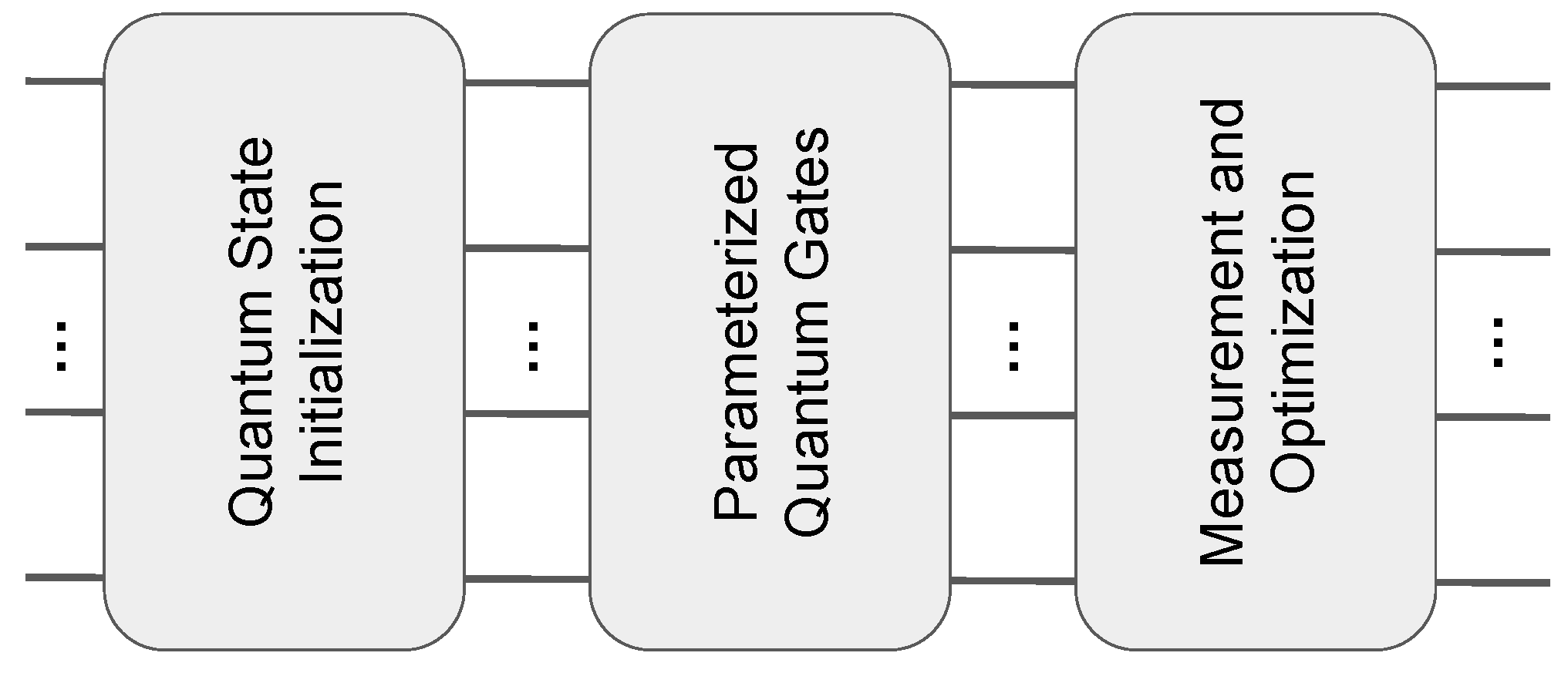
PQC has three main components: quantum state initialization, parameterized quantum gates, and measurement and optimization (Figure 1). In quantum state initialization, each qubit in the circuit is typically set to state $\left|0\right.⟩$, a random state, or a specific initial state. The quantum circuit generally uses multiple layers of parameterized quantum gates, which include adjustable single-qubit rotation gates such as RX, RY, and RZ gates with rotation angles as the trainable parameters, and controlled- and multi-controlled gates such as the CX and CCX gates to form the entanglement of qubits. At the end of the quantum circuit, qubit measurements are performed to obtain the final computation results, which are then used to calculate the loss function values. These calculation results are then fed to a classical machine learning optimizer to optimize and minimize loss function values so that PQC can generate desirable outputs.

2.3. Data Imbalance and Resampling

In machine learning, an imbalanced dataset refers to a dataset in which the number of samples for certain labels or classes is significantly larger than the others [15]. For example, in anomaly detection datasets, the amount of normal data are usually larger than that of the abnormal data. Imbalanced datasets cause the data imbalance issue, biasing models, as most machine learning algorithms assume an equal distribution of classes. As a result, the model becomes accurate at predicting the majority class but performs poorly for the minority class, which is critical in applications like anomaly detection.

To address the data imbalance issue, we adopted data resampling techniques, including random oversampling, random undersampling, SMOTE, and T-link undersampling.

Random oversampling is used to balance class distribution by increasing the number of minority class samples and randomly duplicating existing samples from the minority class until they match the number of majority class samples [8]. As oversampling does not remove any samples, no information from the original dataset is lost. Random undersampling balances the ratio of class samples by reducing the number of majority class samples [8]. Samples are randomly selected and removed from the majority class until their number matches that of the minority class samples. The purpose is to prevent the model from being overly biased toward the majority class, thereby improving its ability to distinguish minority classes. By reducing the number of majority class samples, the dataset’s size is decreased, which shortens the training and prediction times and helps prevent the model from overfitting to the majority class.

SMOTE is widely used for handling imbalanced datasets to balance class distribution by generating synthetic minority class samples [9]. Unlike random oversampling, SMOTE increases dataset diversity by interpolating samples in the feature space to synthesize new samples, reducing the risk of overfitting. The process of SMOTE is described as follows.

First, a sample x_i is selected from the minority class, and a value k is set to find the k nearest neighbors of minority class samples of x_i. One of these nearest neighboring samples x_nn is chosen, and a new sample x_new is generated between x_nn and x_i, which is then added to the minority class. The new sample x_new is calculated as

$$x_{new}=x_i+\lambda \cdot \left(x_{nn}-x_i\right),$$

(3)

where $\lambda$ is a random number between 0 and 1.

T-link is used to handle imbalanced datasets by cleaning noisy and borderline samples in the majority class, thereby improving the performance of classification models [10]. The basic idea of T-link is described as follows. Specific T-link pairs of nearest samples are first formed. A pair (x, y) of samples x and y is a T-link pair if the following conditions are satisfied.

When x and y belong to different classes, no third sample z exists in d(x, z) < d(x, y) or d(y, z) < d(y, x), where d(·) is the Euclidean distance between samples in the feature space. In other words, a T-link pair is a nearest-neighbor pair between different classes. Removing the majority of class samples from T-link pairs makes the boundary between classes distinct and clear, which improves the classification performance.

2.4. Autoencoder

An autoencoder (AE) is a special neural network model designed to learn efficient representations of data [12]. It consists of three main components: the encoder, the code, and the decoder. The encoder compresses the high-dimensional input data into the code for a lower-dimensional latent representation. This process is akin to dimensionality reduction, where the compressed representation captures the most important features of the original data in a more compact form. The decoder then reconstructs the data from the code in the low-dimensional latent space to reconstruct an output as close as possible to the original input. The training objective of AE is to minimize the error between the input data and the reconstructed output, often using mean squared error (MSE) as the loss function. Through the training process, AE represents the key features of the high-dimensional data with the low-dimensional codes in the latent space.

2.5. Isolation Forest

Isolation forest (IF) is an unsupervised machine learning model designed for anomaly detection [13]. IF is based on the observation that anomalies are few and distinct from normal samples, making them easier to isolate. The IF model randomly selects a feature and partitions the samples recursively. Anomalies, being different from majority class samples, are isolated quickly with fewer splits, whereas normal samples require more splits to separate them from others. The IF model builds multiple decision trees or isolation trees, where each tree is created by recursively splitting the data samples. Each sample’s anomaly score is determined by the number of splits (or path length) taken to isolate it. Samples with shorter path lengths are likely to be anomalies, as they are isolated faster, whereas samples that require more splits are considered normal. The IF model is computationally efficient and is appropriate for large, high-dimensional datasets, making it ideal for detecting anomalies in complex data.

3. Methodology

We used PQC for anomaly detection (Figure 2). PQC comprises the encoding layer, quantum gate layer, and measurement layer. The encoding layer uses the “amplitude embedding” to encode classical data into quantum states. Amplitude embedding stores N-dimensional data with the superposition state $\left|\psi \right.⟩$ of n qubits, where N = 2ⁿ. The number n of qubits must be selected appropriately so that the number of data points is less than or equal to N = 2ⁿ. Specifically, each classical data point is normalized to be x_i to satisfy the following equation.

$$\sum _{i=0}^{N-1}{\left|x_i\right|}^2=1.$$

(4)

Normalization is performed by calculating the sum S of squares of the original data points and dividing each data point by $\sqrt{s}$ to obtain the normalized data points. When x_i is the probability of the corresponding basis state $\left|i\right.⟩$, $0\le i\le {N-1=2}^n-1$, and

$$\left|\psi \right.⟩=\sum _{i=0}^{N-1}{x}_i\left|i\right.⟩$$

(5)

The quantum gate layer is included in the quantum circuit [16]. As shown in Figure 2, each qubit in the quantum circuit passes through a parameterized rotation quantum gate, which includes RX, RY, and RZ gates. Then, it goes through a series of CX gates to ensure that the qubits become entangled with each other.

The final measurement layer is responsible for measuring the outcomes, and the results of the qubit measurements are represented probabilistically as real numbers between 0 and 1. In Figure 2, only one qubit is measured. The measurement result is the probability of the qubit to be $\left|1\right.⟩.$ For detecting anomalies, if the probability is greater than 0.5, it is interpreted as a normal sample; otherwise, it is an anomaly sample. The proposed PQC in this study does not address the data imbalance issue, so it is necessary to investigate the performance differences when using and not using resampling techniques. The resampling techniques include random oversampling, random undersampling, SMOTE oversampling, and T-link undersampling. The resampled data were fed to PQC to detect anomalies.

4. Results

In this study, we used PennyLane [17] to design and simulate PQC for anomaly detection. PennyLane is a framework developed by Xanadu Quantum Technologies, Toronto, Canada. It is designed for integrating quantum computing with classical machine learning tools for designing and simulating PQC. PennyLane supports a variety of quantum hardware backends (e.g., IBM Q, Rigetti Aspen, Honeywell, and IonQ quantum computers) and simulators (e.g., IBM Qiskit Aer, Rigetti Forest QVM, Google Cirq, Amazon Braket Local Simulator, TensorFlow Quantum, and PyTorch Quantum). It seamlessly integrates with classical optimizers, e.g., the gradient descent optimizer, Adam optimizer, conjugate gradient optimizer, Nelder−Mead, Powell, and constrained optimization by linear approximations (COBYLA) derivative-free optimizers, and simultaneous perturbation stochastic approximation (SPSA) optimizer, to efficiently tune the parameters of PQC. One of PennyLane’s key advantages is its built-in automatic differentiation feature, which simplifies the process of calculating PQC gradients. It leverages the “parameter-shift rule” for efficient gradient computation, allowing users to automatically handle gradient updates while adjusting PQCs. This accelerates the PQC training process and enhances the accuracy of the simulations.

We used the Musk dataset [11] from the University of California, Irvine (UCI) machine learning repository to evaluate the performance of PQC. Musk is a dataset for molecular classification that includes 166 integer-type features of molecules to predict whether a molecule has the Musk property. In the Musk1 and Musk2, 476 and 6598 samples are included, respectively. We used the Musk2 dataset, where 5581 samples were labeled as non-musk.

Samples in the dataset were labeled as Musk or Non-musk, making it a commonly used benchmark dataset for binary classification in machine learning. The dataset is imbalanced in anomaly detection scenarios. This is why we used the dataset for outlier (or anomaly) detection.

We adopted the well-known classical Adam (adaptive moment estimation) optimizer to tune the PQC parameters. Adam is based on gradient descent and is beneficial with the built-in automatic differentiation provided by PennyLane. We used MSE as the loss function, set the number of epochs to 80, and applied five-fold cross-validation in the training process. To ensure fair comparisons, all models were set with the same hyperparameters mentioned above.

We used the F1 score to evaluate the performance of PQC and other models for comparisons. The F1score is a metric for assessing classification models, incorporating precision and recall. It is the harmonic mean of these two metrics, and its related formulas are as follows:

$$\mathrm{F}1-\mathrm{score}=2\times {\displaystyle \frac{\mathrm{p}\mathrm{r}\mathrm{e}\mathrm{c}\mathrm{i}\mathrm{s}\mathrm{i}\mathrm{o}\mathrm{n}\times \mathrm{r}\mathrm{e}\mathrm{c}\mathrm{a}\mathrm{l}\mathrm{l}}{\mathrm{p}\mathrm{r}\mathrm{e}\mathrm{c}\mathrm{i}\mathrm{s}\mathrm{i}\mathrm{o}\mathrm{n}+\mathrm{r}\mathrm{e}\mathrm{c}\mathrm{a}\mathrm{l}\mathrm{l}}}$$

(6)

$$\mathrm{precision}={\displaystyle \frac{\mathrm{T}\mathrm{P}}{\mathrm{T}\mathrm{P}+\mathrm{F}\mathrm{P}}}$$

(7)

$$\mathrm{recall}={\displaystyle \frac{\mathrm{T}\mathrm{P}}{\mathrm{T}\mathrm{P}+\mathrm{F}\mathrm{N}}}$$

(8)

In Equations (7) and (8), TP, FP, TN, and FN stand for the numbers of true positive, false positive, true negative, and false negative detections, respectively.

The output of PQC was derived by running the circuit using a PennyLane simulator. The output of PQC was represented as the probability of the measurement result of 1 in a continuous range [0, 1]. However, in the Musk dataset, the labels are discrete and are either 0 or 1. Therefore, the output of PQC was adjusted as follows. If the output probability is greater than 0.5, it is interpreted as 1 (indicating a normal label), and if it is less than or equal to 0.5, it is interpreted as 0 (indicating an anomaly label).

We experimented with the PQC model without or with data resampling methods, such as random oversampling, random undersampling, SMOTE, and T-link. We also experimented with the classical state-of-the-art method, which is the combination of the autoencoder and the isolation forest, without data resampling.

Table 1. Comparisons in terms of F1 scores for models with or without data resampling.

Methodology		F1-Score
Preprocessing	Model	Train/Test	1st Exp.	2nd Exp.	Avg.
AutoEncoder	Isolation Forest	train	0.7269	0.7319	0.7294
		test	0.7470	0.7180	0.7325
No Resampling	PQC	train	0.5986	0.5985	0.5986
		test	0.5921	0.5761	0.5841
Random Oversampling		train	0.6911	0.6183	0.6547
		test	0.6453	0.5946	0.6200
SMOTE Oversampling		train	0.6688	0.6490	0.6589
		test	0.6024	0.6475	0.6250
Random Undersampling		train	0.6984	0.6986	0.6985
		test	0.6552	0.6807	0.6680
Tomek Link Undersampling		train	0.8357	0.6666	0.7512
		test	0.7178	0.6635	0.6907

shows the comparison results for all methodologies with or without data preprocessing (or resampling). As we used a quantum simulator for training the PQC, each training process took about 10 h. To save time, we averaged the results of only two experiments for each methodology for the comparisons. When no resampling technique was applied, PQC had an average F1 score of only 0.5841. However, after applying resampling techniques, the average F1 score exceeded 0.62 and reached 0.6907. This showed a noticeable performance improvement of PQC when resampling techniques were applied.

When comparing the four resampling techniques, SMOTE and T-link performed better than random oversampling and random undersampling, suggesting that SMOTE and T-link were more effective at handling data imbalance than random resampling methods. Undersampling techniques outperformed oversampling techniques, as oversampling introduces noisy samples, which negatively impact model performance.

When comparing PQC with classical methods and the combination of the autoencoder and the isolation forest, the latter presented a performance advantage. In the noisy intermediate-scale quantum (NISQ) era, real quantum computers produce incorrect results due to noise. Therefore, we used simulators to execute PQC. The simpler the PQC designs, the better the performance. Additionally, as running quantum circuits on simulators is time-consuming, the efficient tuning of PQC hyperparameters is required for the performance of PQC.

5. Conclusions

We applied PQC to anomaly detection to improve the performance by employing different resampling techniques, including random oversampling, random undersampling, SMOTE oversampling, and T-link undersampling. The experimental results showed noticeable improvements in the F1 score of PQC after applying resampling techniques, with SMOTE and T-link showing a better performance than their randomized counterparts, indicating their advantages in handling imbalanced data. Oversampling techniques performed worse than undersampling techniques, possibly due to the introduction of noise samples in the oversampling process, which negatively impacted the model performance. Regardless of the resampling technique, the performance of PQC was inferior to traditional methods, specifically the combination of an autoencoder and an isolation forest. The autoencoder effectively extracts features while the isolation forest is inherently less sensitive to data imbalance and needs no data resampling. Additionally, in the NISQ era, real quantum computers might produce incorrect results due to noise. Therefore, it is necessary to use simulators to execute PQC. This necessitates simpler PQC designs, which affects the PQC performance. Moreover, running the PQC on simulators is time-consuming, preventing efficient tuning of PQC hyperparameters, which further negatively impacts the performance of PQCs.

In the future, it is necessary to investigate complex PQC models [16] for anomaly detection and explore different types of quantum machine learning models [18] to improve anomaly detection performance. The quantum machine learning models explored include the quantum support vector machine [19] and the quantum random forest [20], both of which are less sensitive to imbalanced data and are expected to perform well in anomaly detection.