
Calculating Percentiles of T-Distribution Using Gaussian Integration Method †

Abstract
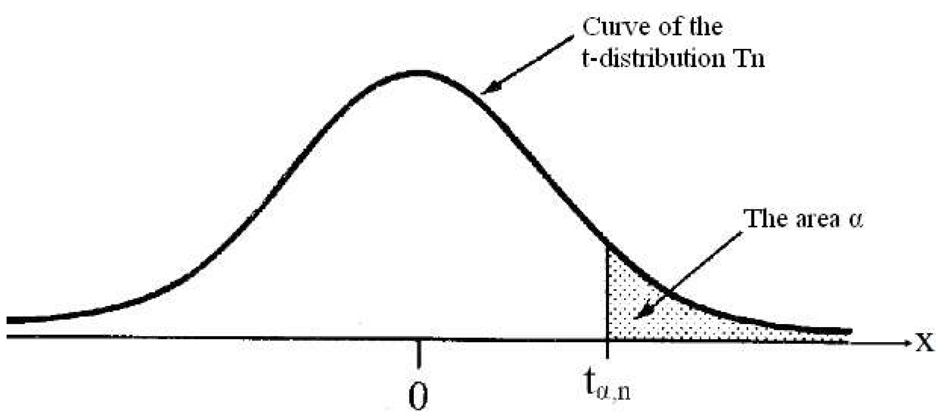
1. Introduction
2. Gaussian Integration Method
3. Evaluation Percentiles of T-Distribution
4. Conclusions
Funding
Institutional Review Board Statement
Informed Consent Statement
Data Availability Statement
Conflicts of Interest
References
- Montgomery, D.C. Design and Analysis of Experiments; John Wiley & Sons: New York, NY, USA, 2001. [Google Scholar]
- Lee, J.B.; Max, E. Introduction to Probability and Mathematical Statistics; Duxbury Press: Belmont, CA, USA, 1992. [Google Scholar]
- Jay, L.D. Probability and Statistics for Engineering and the Sciences; Brooks/Cole: Pacific Grove, CA, USA, 2012. [Google Scholar]
- Zienkiewicz, O.C. The Finite Element Method; McGraw-Hill Book Co.: Maidenhead, UK, 1977. [Google Scholar]
- Bathe, K.J. Finite Element Procedures in Engineering Analysis; Prentice-Hall: Upper Saddle River, NJ, USA, 1982. [Google Scholar]
- Pearson, E.S.; Hartley, H.O. Biometrika Tables for Statisticians; Cambridge University Press: Cambridge, UK, 1966. [Google Scholar]

| Number of Sampling Points (m) | Sampling Points (wi) | Weighting Coefficients (λi) |
|---|---|---|
| 1 | 0.0 | 2.0 |
| 2 | λ1 = −0.57735 02691 89626 | w1 = 1.0 |
| λ2 = 0.57735 02691 89626 | w2 = 1.0 | |
| 3 | λ1 = −0.77459 66692 41483 | w1 = 0.55555 55555 55556 |
| λ2 = 0.00000 00000 00000 | w2 = 0.88888 88888 88889 | |
| λ3 = 0.77459 66692 41483 | w3 = 0.55555 55555 55556 | |
| 4 | λ1 = −0.86113 63115 94053 | w1 = 0.34785 48451 37454 |
| λ2 = −0.33998 10435 84856 | w2 = 0.65214 51548 62546 | |
| λ3 = 0.339981043584856 | w3 = 0.65214 51548 62546 | |
| λ4 = 0.861136311594053 | w4 = 0.34785 48451 37454 | |
| 5 | λ1 = −0.90617 98459 38664 | w1 = 0.23692 68850 56189 |
| λ2 = −0.53846 93101 05683 | w2 = 0.47862 86704 99366 | |
| λ3 = 0.00000 00000 00000 | w3 = 0.56888 88888 88889 | |
| λ4 = 0.53846 93101 05683 | w4 = 0.47862 86704 99366 | |
| λ5 = 0.90617 98459 38664 | w5 = 0.23692 68850 56189 | |
| 6 | λ1 = −0.93246 95142 03152 | w1 = 0.17132 44923 79170 |
| λ2 = −0.66120 93864 66265 | w2 = 0.36076 15730 48139 | |
| λ3 = −0.23861 91860 83197 | w3 = 0.46791 39345 72691 | |
| λ4 = 0.23861 91860 83197 | w4 = 0.46791 39345 72691 | |
| λ5 = 0.66120 93864 66265 | w5 = 0.36076 15730 48139 | |
| λ6 = 0.93246 95142 03152 | w6 = 0.17132 44923 79170 |
| Degrees of Freedom n | ||||
|---|---|---|---|---|
| 0.200 | 0.100 | 0.050 | 0.025 | |
| 1 | 1.3764 | 3.0777 | 6.3138 | 12.7062 |
| 2 | 1.0607 | 1.8856 | 2.9200 | 4.3027 |
| 3 | 0.9785 | 1.6377 | 2.3534 | 3.1824 |
| 4 | 0.9410 | 1.5332 | 2.1318 | 2.7764 |
| 5 | 0.9195 | 1.4759 | 2.0150 | 2.5706 |
| 6 | 0.9057 | 1.4398 | 1.9432 | 2.4469 |
| 7 | 0.8960 | 1.4149 | 1.8941 | 2.3646 |
| 8 | 0.8889 | 1.3968 | 1.8595 | 2.3060 |
| 9 | 0.8834 | 1.3830 | 1.8331 | 2.2622 |
| 10 | 0.8791 | 1.3722 | 1.8125 | 2.2281 |
| 15 | 0.8662 | 1.3406 | 1.7531 | 2.1315 |
| 20 | 0.8600 | 1.3253 | 1.7247 | 2.0860 |
| 30 | 0.8538 | 1.3104 | 1.6973 | 2.0423 |
| 40 | 0.8507 | 1.3031 | 1.6839 | 2.0211 |
| 60 | 0.8477 | 1.2958 | 1.6706 | 2.0003 |
| 80 | 0.8461 | 1.2922 | 1.6641 | 1.9901 |
| 100 | 0.8452 | 1.2901 | 1.6602 | 1.9840 |
| 120 | 0.8446 | 1.2886 | 1.6577 | 1.9799 |
| Degrees of Freedom n | ||||
| 0.010 | 0.005 | 0.001 | 0.0005 | |
| 1 | 31.8205 | 63.6567 | 318.3088 | 636.6192 |
| 2 | 6.9646 | 9.9248 | 22.3271 | 31.5991 |
| 3 | 4.5407 | 5.8409 | 10.2145 | 12.9240 |
| 4 | 3.7469 | 4.6041 | 7.1732 | 8.6103 |
| 5 | 3.3649 | 4.0321 | 5.8934 | 6.8688 |
| 6 | 3.1427 | 3.7074 | 5.2076 | 5.9588 |
| 7 | 2.9980 | 3.4995 | 4.7853 | 5.4079 |
| 8 | 2.8965 | 3.3554 | 4.5008 | 5.0413 |
| 9 | 2.8214 | 3.2498 | 4.2968 | 4.7809 |
| 10 | 2.7638 | 3.1693 | 4.1437 | 4.5869 |
| 15 | 2.6025 | 2.9467 | 3.7328 | 4.0728 |
| 20 | 2.5280 | 2.8453 | 3.5518 | 3.8495 |
| 30 | 2.4573 | 2.7500 | 3.3852 | 3.6460 |
| 40 | 2.4233 | 2.7045 | 3.3069 | 3.5510 |
| 60 | 2.3901 | 2.6603 | 3.2317 | 3.4602 |
| 80 | 2.3739 | 2.6387 | 3.1953 | 3.4163 |
| 100 | 2.3642 | 2.6259 | 3.1737 | 3.3905 |
| 120 | 2.3578 | 2.6174 | 3.1595 | 3.3735 |
| NSECT | NSECT | ||
|---|---|---|---|
| 100 | 574.327106 | 2500 | 636.619249 |
| 175 | 489.829447 | 5000 | 636.619249 |
| 250 | 599.936222 | 636.619249 | |
| 500 | 635.953237 | 636.619249 | |
| 750 | 636.635366 | 636.619249 | |
| 1000 | 636.621221 | 636.619249 |
| NSECT | NSECT | ||
|---|---|---|---|
| 100 | −0.000585 | 2500 | 0.000500 |
| 175 | 0.000895 | 5000 | 0.000500 |
| 250 | 0.000527 | 0.000500 | |
| 500 | 0.000499 | 0.000500 | |
| 750 | 0.000500 | 0.000500 | |
| 1000 | 0.000500 | 0.000500 |
Disclaimer/Publisher’s Note: The statements, opinions and data contained in all publications are solely those of the individual author(s) and contributor(s) and not of MDPI and/or the editor(s). MDPI and/or the editor(s) disclaim responsibility for any injury to people or property resulting from any ideas, methods, instructions or products referred to in the content. |
© 2025 by the author. Licensee MDPI, Basel, Switzerland. This article is an open access article distributed under the terms and conditions of the Creative Commons Attribution (CC BY) license (https://creativecommons.org/licenses/by/4.0/).
Share and Cite
Tien, T.-L. Calculating Percentiles of T-Distribution Using Gaussian Integration Method. Eng. Proc. 2025, 92, 2. https://doi.org/10.3390/engproc2025092002
Tien T-L. Calculating Percentiles of T-Distribution Using Gaussian Integration Method. Engineering Proceedings. 2025; 92(1):2. https://doi.org/10.3390/engproc2025092002
Chicago/Turabian StyleTien, Tzu-Li. 2025. "Calculating Percentiles of T-Distribution Using Gaussian Integration Method" Engineering Proceedings 92, no. 1: 2. https://doi.org/10.3390/engproc2025092002
APA StyleTien, T.-L. (2025). Calculating Percentiles of T-Distribution Using Gaussian Integration Method. Engineering Proceedings, 92(1), 2. https://doi.org/10.3390/engproc2025092002