Assessing Asymptotic Tail Independence: A Simulation Study ^†

Abstract

The occurrence of extreme values in one variable can trigger the same in other variables, making it necessary to assess the risk of contagion. The usual dependence measures based on the central part of the data typically fail to assess extreme dependence. Within the scope of EVT, tail dependence measures were developed, such as the Ledford and Tawn coefficient that we discuss here. This is a measure of residual dependence that is particularly important when it comes to analyzing at the tail level where data are scarce. We will consider different estimation methodologies and compare them based on a simulation study. We finish with an application to real data.

1. Introduction

Applications of EVT in the analysis of risky events are diverse, such as finance, insurance, material resistance, quality control, telecommunications, sports, environment, hydrology, biology, and seismology, among others.

The occurrence of extreme observations can have serious consequences, e.g., high water levels in floods, a vast area burned in wildfires, and losses in stock indexes in financial market crashes, among others. Sometimes, the occurrence of extreme values for one variable can contaminate other variables. Typical examples are the financial markets where the fall of one index leads to falls in others as well. Correlation is a measure of dependence between two variables widely used in applications. Although it works well to measure the association between two variables in the central part of the data, it fails to assess dependence within the tails. For instance, in a bivariate Normal with correlation $\rho <1$, if we are far enough in the tail, extreme values seem to occur independently at each margin, regardless of how high a correlation we choose [1].

Extremal dependence in a random pair $(X,Y)$ is typically based on the chance for obtaining large values of both variables. It is helpful to remove the influence of marginal aspects by transforming the marginals to a common distribution function (df), e.g., $F_X\left(X\right)$ and $F_Y\left(Y\right)$, both of which are standard uniform where $F_X$ and $F_Y$ are the marginal df of X and Y, respectively, and considered continuous. Therefore, differences in distributions are solely due to dependence aspects. As $F_X\left(X\right)$ and $F_Y\left(Y\right)$ are on a common scale, events of the form $\{F_X\left(X\right)>u\}$ and $\{F_Y\left(Y\right)>u\}$, for large values of u, are equally extreme events for each variable, both with their probability approaching zero as $u\to 1$. The tail dependence coefficient (TDC) measures the conditional probability of one variable being extreme, given that the other is extreme too:

$$\begin{array}{c}\hfill {\displaystyle \lambda =\underset{u\to 1}{lim}P(F_X\left(X\right)>u|F_Y\left(Y\right)>u)}\end{array}$$

Observe that the exact independence corresponds to $\lambda =0$, since $P(F_X\left(X\right)>u|F_Y\left(Y\right)>u)=P(F_X\left(X\right)>u)\to 0$, as $u\to 1$, whilst perfect dependence means $P(F_X\left(X\right)>u|F_Y\left(Y\right)>u)=1$. Indeed, we say that X and Y are tail independent if $\lambda =0$, and tail dependent if $\lambda >0$. A positive $\lambda$ means a strong dependence persisting to the limit. A null $\lambda$ comprehends exact independence, but also a weak dependence that gradually vanishes as the limit is approached. Such residual dependency can be captured through the rate of convergence of $P(F_X\left(X\right)>u|F_Y\left(Y\right)>u)$ towards zero; more precisely, through the asymptotic tail independent coefficient of Ledford and Tawn $\eta \in (0,1]$ [2], given by

$$\begin{array}{c}\hfill P(F_X\left(X\right)>u|F_Y\left(Y\right)>u)\sim {(1-u)}^{1/\eta -1}\mathcal{L}(1/(1-u)),u\to 1\end{array}$$

(1)

where $\mathcal{L}\left(x\right)$ is a slowly varying function, i.e., $\mathcal{L}\left(tx\right)/\mathcal{L}\left(x\right)\to 1$, as $x\to \infty$, $t>0$ [3]. If $\eta$ = 1 and $\mathcal{L}\to c$, $0<c\le 1$, the random variables (rvs) are asymptotically dependent. On the other hand, if $\eta <1$ or $\eta$=1 and $\mathcal{L}\to 0$, then $\lambda =0$ and the rv are asymptotically independent with degree $\eta$. The case $\eta =1/2$ means near-independence; in particular, exact independence if $\mathcal{L}\equiv 1$. We can also state that $1/2<\eta <1$ corresponds to a positive association, in the sense that the probability of both rvs exceeding u occurs more frequently than under exact independence, whereas in $0<\eta <1/2$, the probability of both rvs exceeding u occur less frequently than under exact independence and, thus, the rvs are negatively associated. Inference on $\eta$ allows us to distinguish the type of tail (in)dependence: $\eta =1$ means tail dependence, whilst $\eta <1$ means the presence of a residual tail dependence. According to [2], assuming independence and ignoring $\eta$ can lead to misspecified joint extremes estimations, while considering the dependence between rvs, when a residual dependence in fact occurs, may result in an overestimation.

Observe that

$$\begin{array}{c}\hfill P(F_X\left(X\right)>u,F_Y\left(Y\right)>u)=P(U>{(1-u)}^{-1},V>{(1-u)}^{-1})\end{array}$$

where $U={(1-F_X\left(X\right))}^{-1}$ and $V={(1-F_Y\left(Y\right))}^{-1}$ are standard Pareto. Considering rv $T=min(U,V)$ and $t_u={(1-u)}^{-1}$, by (1) we can state that

$$\begin{array}{c}\hfill P(T>t_u)\sim t_u^{-1/\eta }\mathcal{L}\left(t_u\right),t_u\to \infty \end{array}$$

(2)

and we say that T has a regularly varying tail with index $-1/\eta$. In EVT, this means that $\eta$ corresponds to the tail index of T, the primary measure in EVT inference. There are many estimation methods in the literature for the tail index. For a survey, see, e.g., [4]. A well-known tail index estimator is the Hill [5]. Given a sample $T_1,\dots ,T_n$, consider

$$\begin{array}{c}\hfill {\widehat{\eta }}_u^{\left(H\right)}:={\displaystyle \frac{1}{n_u}}\sum _{j=1}^{n_u}log(T_{\left(j\right)}/t_u),\end{array}$$

where $T_{\left(j\right)}$, $j=1,\dots ,n_u$, are the rvs exceeding the threshold $t_u$. In the Hill estimator, $t_u$ corresponds to the $n_u+1$ up order statistics. In EVT, we can also estimate the tail index through a modeling approach. A common technique is to consider the exceedance values above a high threshold of data, and apply a Generalized Pareto Distribution (GPD) according to the Pickands–Balkema–De Haan theorem [6,7], known as the Peaks Over Threshold (POT) approach (see, e.g., [4] for more details). Here, we apply the POT method on rv T in order to estimate $\eta$, and denote this estimator as ${\widehat{\eta }}_u^{\left(GPD\right)}$.

Based on (1), we can rewrite

$$\begin{array}{c}\hfill \eta \equiv \eta \left(u\right)\sim {\displaystyle \frac{log(1-u)}{logP(F_X\left(X\right)>u,F_Y\left(Y\right)>u)}}\end{array}$$

(3)

and, thus, we can estimate $\eta$ by taking the empirical counterpart of (3), which we denote as ${\widehat{\eta }}^{\left(emp\right)}$. More precisely,

$$\begin{array}{c}\hfill {\widehat{\eta }}_u^{\left(emp\right)}\sim {\displaystyle \frac{log(1-u)}{log\left(n^{-1}{\sum }_{i=1}^n{\mathbf{1}}_{\{F_X\left(X_i\right)>u,F_Y\left(Y_i\right)>u\}}\right)}}.\end{array}$$

(4)

Note that, in practice, the margins $F_X$ and $F_Y$ are usually unknown, and we can estimate by the empirical df. This is the approach followed for estimators ${\widehat{\eta }}_u^{\left(H\right)}$, ${\widehat{\eta }}_u^{\left(GPD\right)}$ and ${\widehat{\eta }}_u^{\left(emp\right)}$. Observe also that the standard uniform rvs, $F_X\left(X_i\right)$ and $F_Y\left(Y_i\right)$, $i=1,\dots ,n$, have r-order statistics Beta($r,n-r+1$) distributed. Thus, replacing the marginal empirical df in (4) with Beta($r,n-r+1$) df, we have the fourth estimator, which we denote as ${\widehat{\eta }}_u^{\left(beta\right)}$. Further details on Beta marginals estimation can be seen in [8].

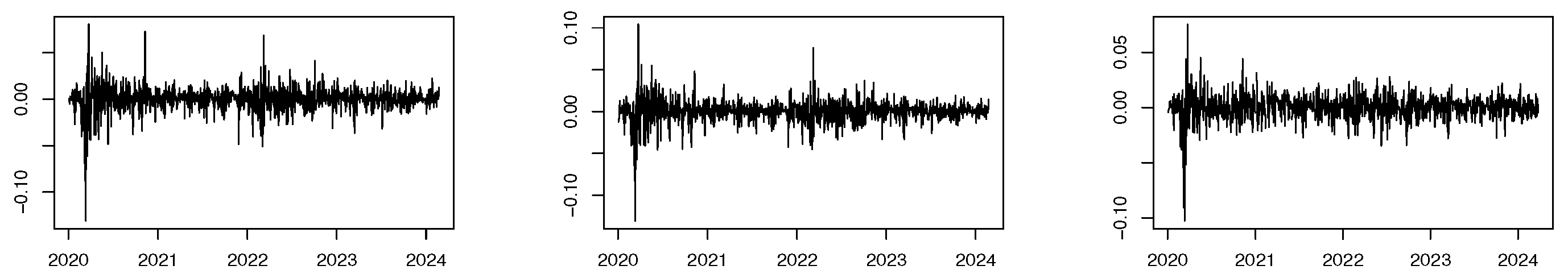
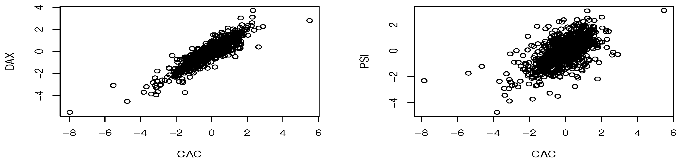
In Section 2, we analyze the referred estimators through simulation and compare their performance. An application to real data illustrates the methods in Section 3.

2. Estimation of $\eta$: A Simulation Study

In our study, we consider different models with different values of $\eta$, as follows, where we use copula notation, $C(u,v)=P(F_X\left(X\right)<u,F_Y\left(Y\right)<v)$:

• Bivariate Ali–Mikhail–Haq distribution, where $C(u,v)=uv{(1-\xi (1-u)(1-v))}^{-1}$, with $\xi =-1$ ($\eta =1/3$) (see, e.g., [9]), denoted AMH;
• Bivariate Frank distribution, where $C(u,v)=-{\xi }^{-1}log(1-(1-e^{-\xi u})(1-e^{-\xi v})/(1-e^{-\xi }))$, with $\xi =0.5$ ($\eta =1/2$) (see, e.g., [9]), denoted Frank;
• Bivariate Normal distribution with $\rho =0.5$ ($\eta =3/4$) (see, e.g., [10]), denoted BNormal;
• Bivariate extreme value distribution with a Logistic dependence function, $C(u,v)=exp\left(-{({(-logu)}^{-1/\alpha }+{(-logv)}^{-1/\alpha })}^{\alpha }\right)$, $0<\alpha \le 1$, with $\alpha =0.75$ ($\eta =1$) (see, e.g., [2]), denoted Logistic.

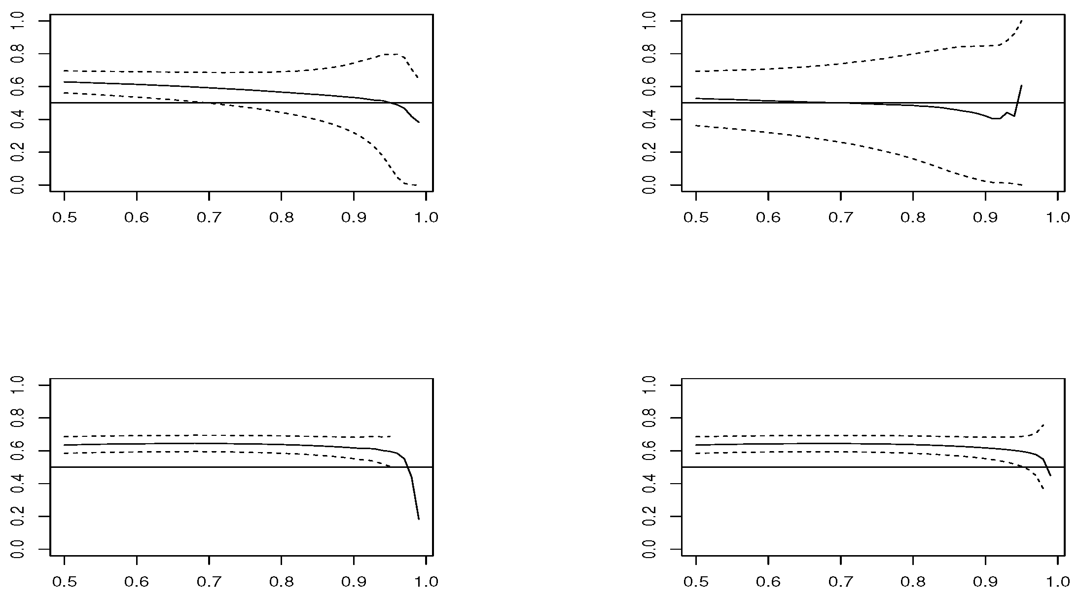
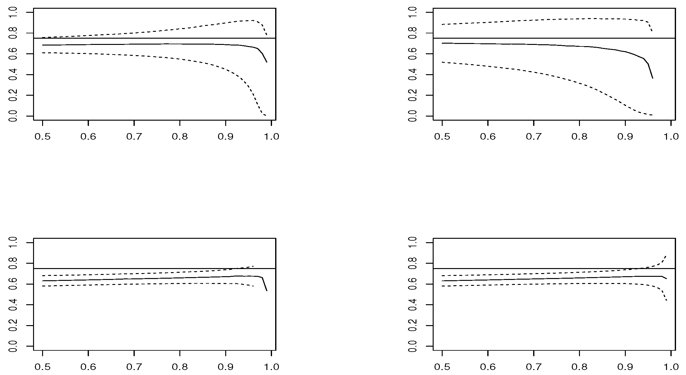
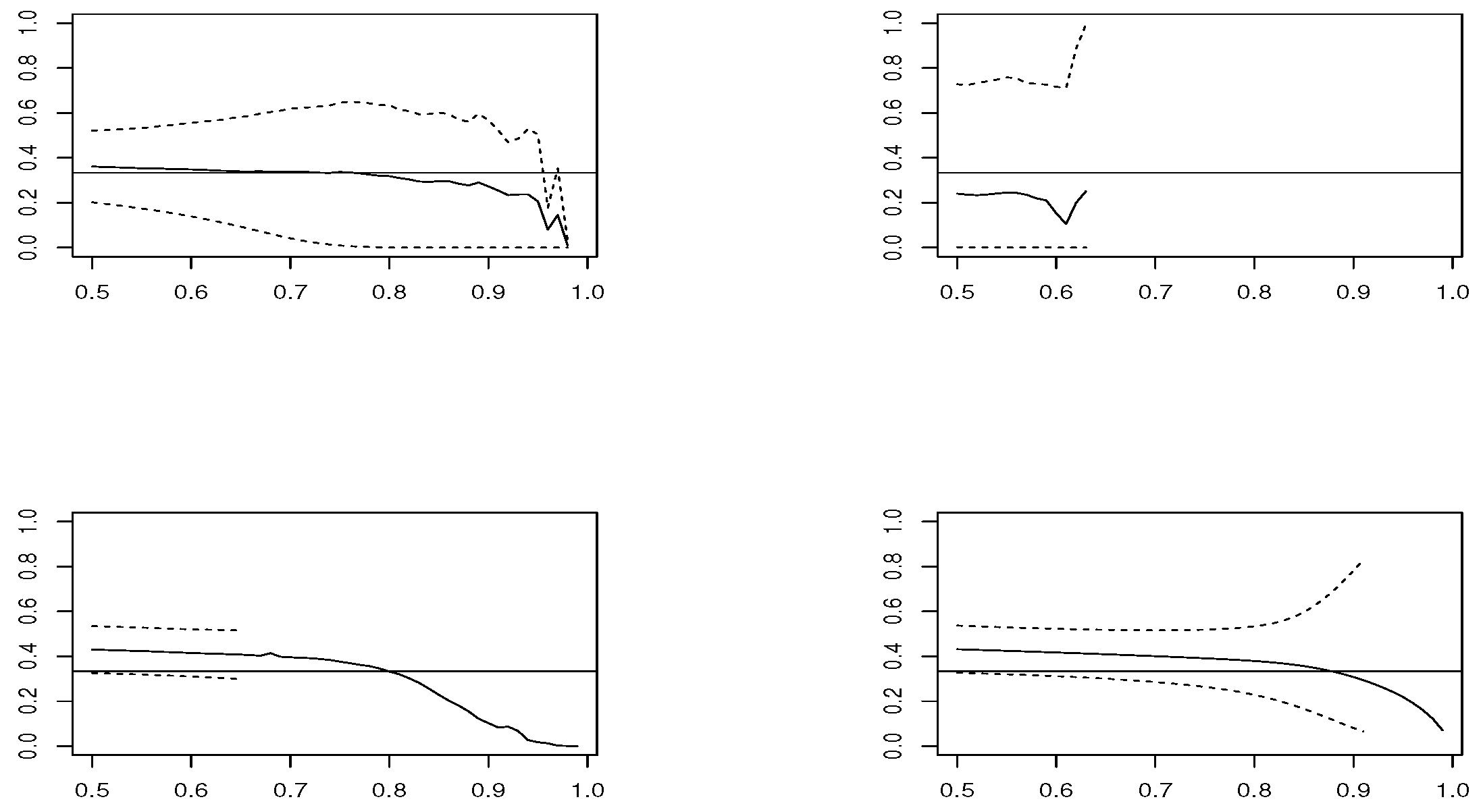
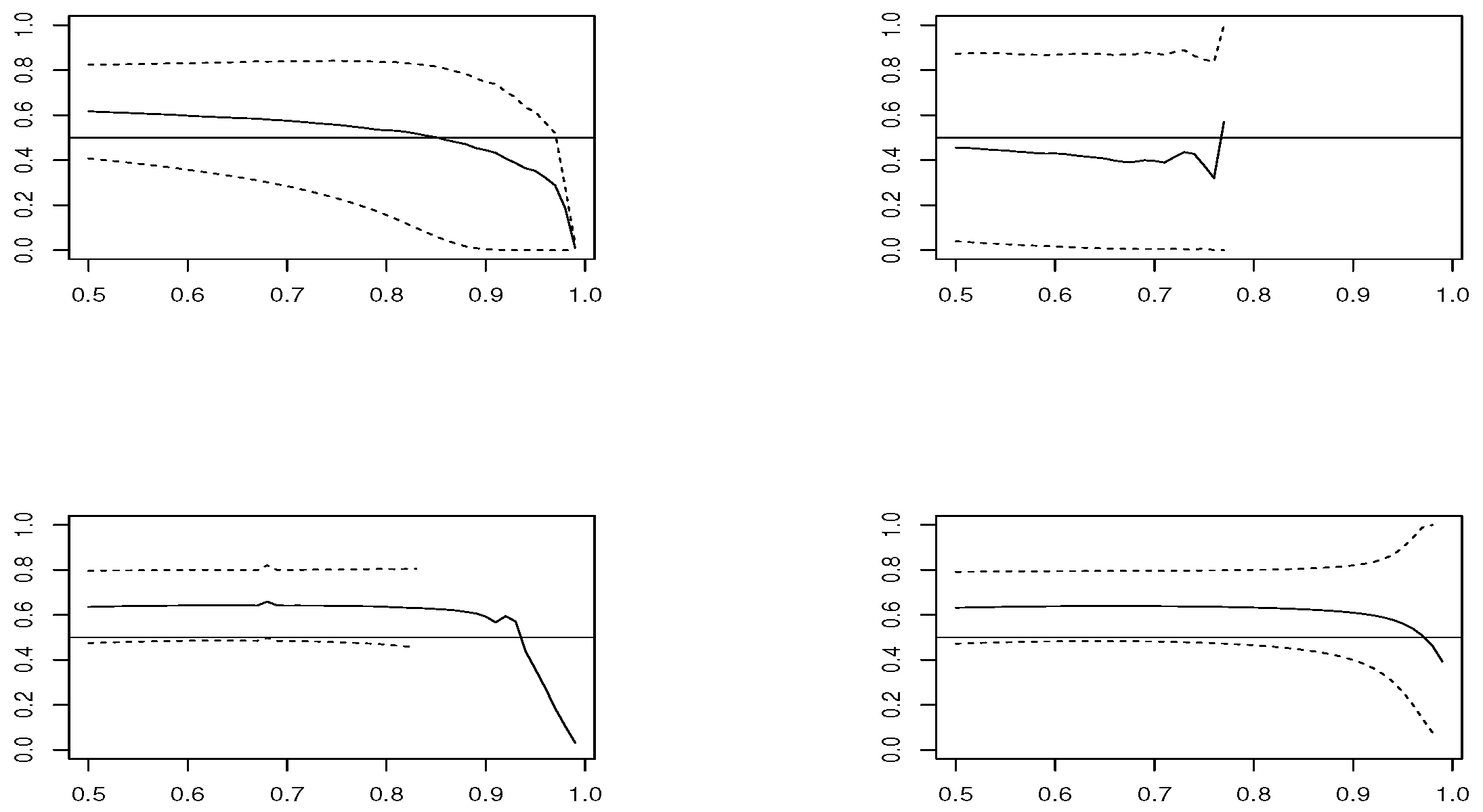
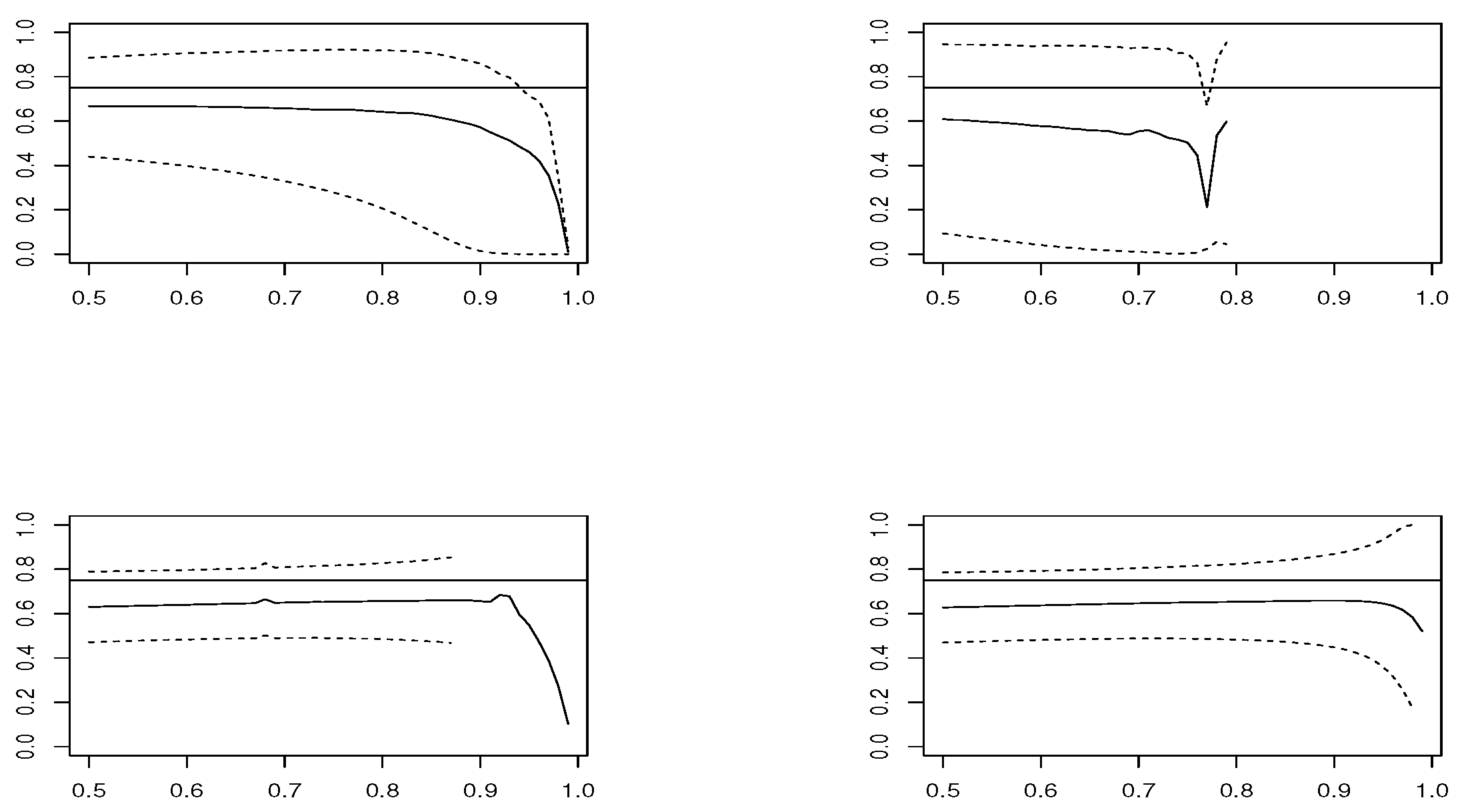
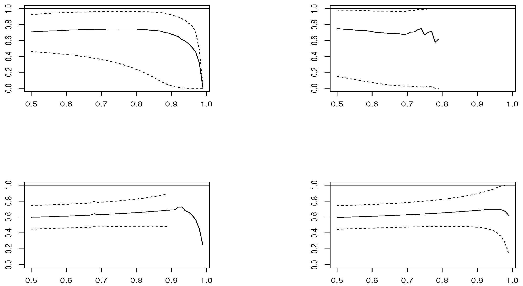
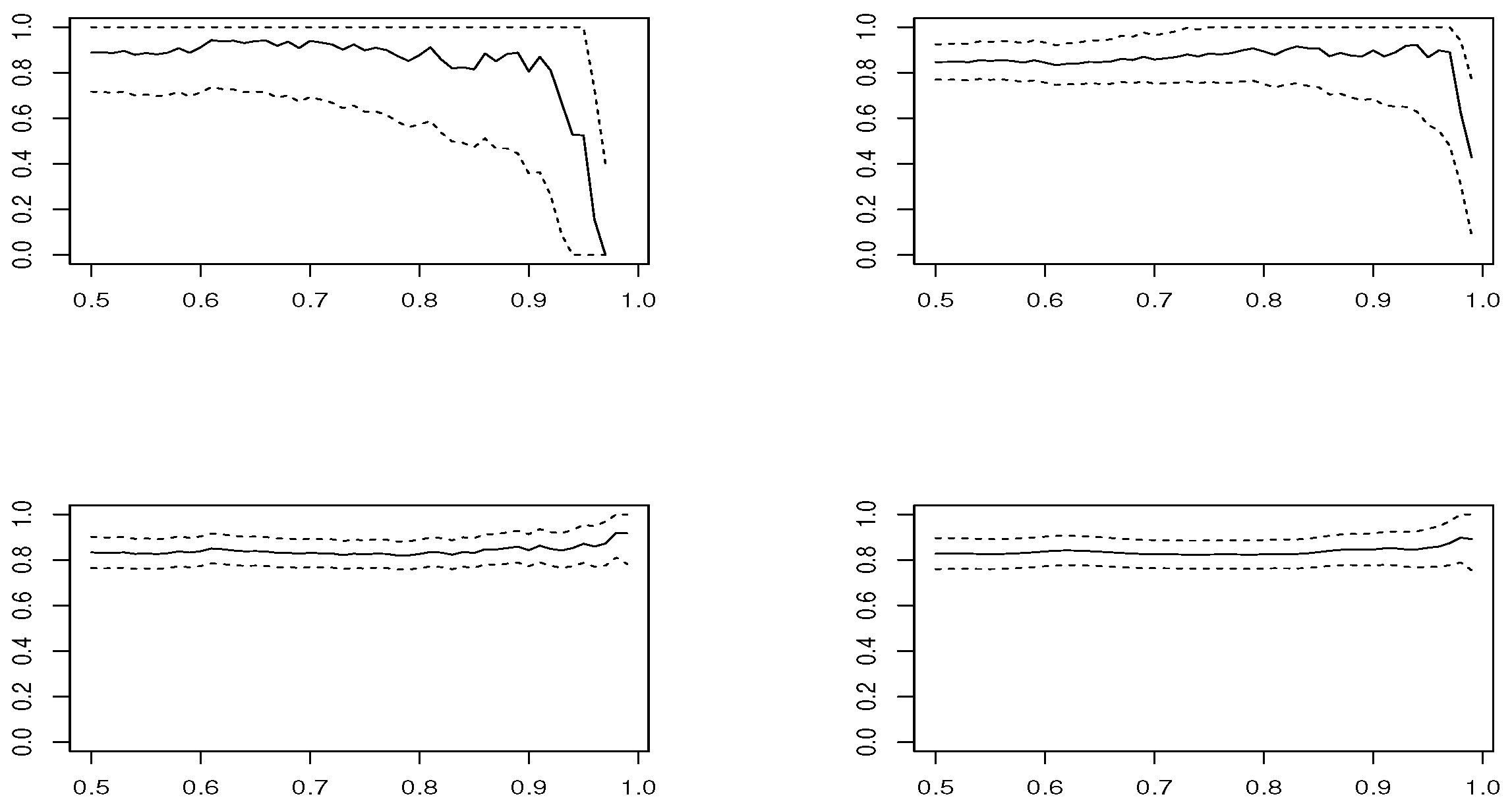
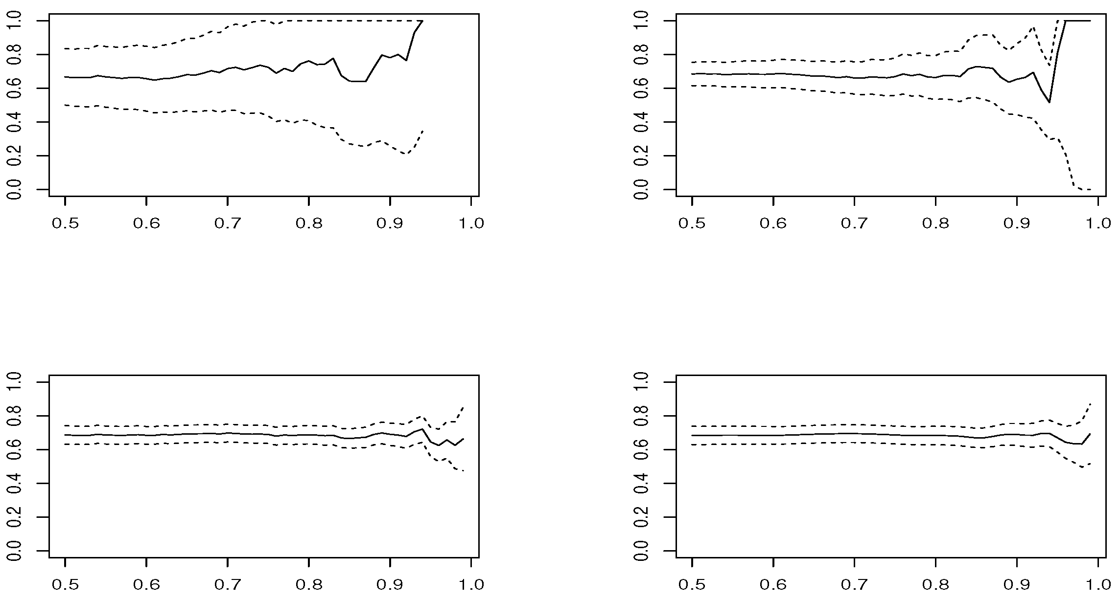
We simulate 1000 replicas of each model, with size $n=100$ and $n=1000$. We compute estimators ${\widehat{\eta }}_u^{\left(H\right)}$, ${\widehat{\eta }}_u^{\left(GPD\right)}$, ${\widehat{\eta }}_u^{\left(emp\right)}$ and ${\widehat{\eta }}_u^{\left(beta\right)}$ for thresholds u corresponding to percentiles $0.5\left(0.01\right)0.99$. The estimation is conducted using package mev [11] within statistical software R 2020 [12]. We derive the sample mean of estimates in each threshold u along with the Wald 95% confidence interval, which are plotted in Figure 1, Figure 2, Figure 3 and Figure 4, in the case of samples with size $n=1000$, and Figure 5, Figure 6, Figure 7 and Figure 8 for $n=100$. 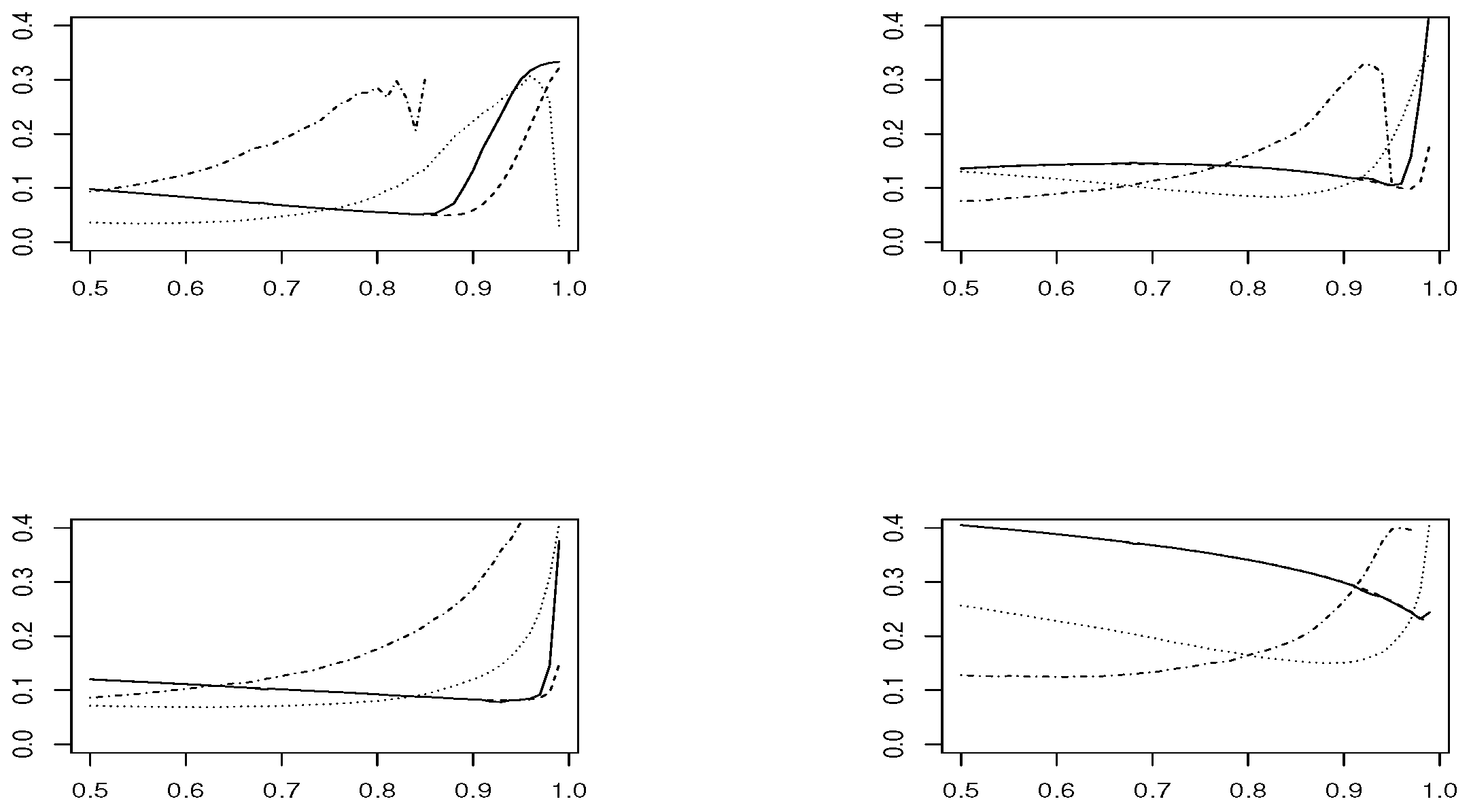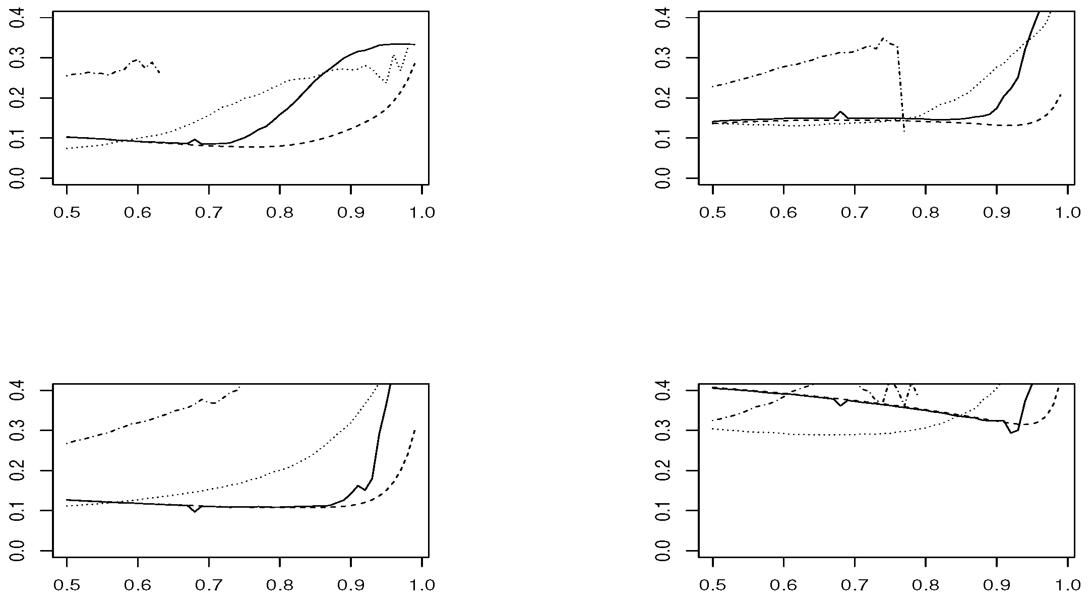We also calculate the root mean squared error (RMSE) in each threshold u, available in Figure 9 and Figure 10, for sample sizes $n=1000$ and $n=100$, respectively. The ${\widehat{\eta }}_u^{\left(GPD\right)}$ estimator is based on modeling threshold exceedances through the GPD model and, therefore, fails to be applied at very high thresholds, where the number of observations is small.

In the case $n=1000$, and looking at the estimated means, estimators ${\widehat{\eta }}_u^{\left(H\right)}$ and ${\widehat{\eta }}_u^{\left(GPD\right)}$ have the best performance. However, concerning the RMSE, ${\widehat{\eta }}_u^{\left(GPD\right)}$ presents the worst performance, except in the Logistic model, where ${\widehat{\eta }}_u^{\left(H\right)}$ and ${\widehat{\eta }}_u^{\left(GPD\right)}$ are the best choices and ${\widehat{\eta }}_u^{\left(emp\right)}$ and ${\widehat{\eta }}_u^{\left(beta\right)}$ are not recommended. In smaller sample size $n=100$, the confidence intervals become larger and the results are less precise. The RMSE grows slightly for all estimators, except for ${\widehat{\eta }}_u^{\left(GPD\right)}$, where it clearly increases. The low performance of all estimators is in the Logistic model, where $\eta =1$ corresponds to a boundary value.

3. Application

We are going to analyze the tail dependence between two stock market indexes pairs, CAC40–DAX and CAC40–PSI20, from January 2020 to February 2024, available from https://finance.yahoo.com/world-indices/ (accessed on 1 March 2024). We consider the daily close log-returns of each index, plotted in Figure 11. In order to remove heteroskedasticity, we apply an asymmetric GARCH filter. The scatter-plot in Figure 12 represents the 1037 pairs of residuals, where the association between the variables is evident, both in the central part and in the tail. The estimates of $\eta$ are plotted in Figure 13 and Figure 14. The value $\eta =1$ seems plausible for the CAC40–DAX pair, particularly in estimators ${\widehat{\eta }}_u^{\left(H\right)}$ and ${\widehat{\eta }}_u^{\left(GPD\right)}$, leading to a diagnostic of tail dependence. Regarding CAC40–PSI20, the $\eta$ estimate is pointed out to be $0.7$, meaning asymptotic tail independence. Therefore, the risk of contagion for the occurrence of extreme values is higher between the CAC40 and DAX indices, when compared with the CAC40–PSI20 pair.

4. Conclusions

In this work, we addressed the inference in tail dependence between two variables, through the Ledford and Tawn coefficient $\eta$ [2]. This is an important parameter in EVT, as it captures the presence of a possible residual dependence that, once ignored, leads to misspecifications. In the context of EVT, where data are scarce and one needs to extrapolate beyond observations, accuracy in estimations is a particularly sensitive topic. There are different methodologies in the literature for estimating $\eta$. In this work, we consider four widely used estimators, and compare their performance in different models. The results obtained constitute an initial guide on the best options for choosing estimators in practical applications. In future work, we intend to continue this study, with more models and variations in $\eta$ values, and thus improve guidance for users in choosing the best estimation method.