A Machine Learning-Based Approach to Analyze and Visualize Time-Series Sentencing Data ^†

Abstract

Analyzing time-series sentencing data presents many challenges. The data have many dimensions and change with time. This makes it difficult to identify patterns and discuss their similarities over time. This work proposes a machine learning approach to associate patterns with clusters. This allows a representation of sentencing data regarding trajectories in the appropriate (time, cluster) space. We propose to use the Hamming distance of trajectories to measure the similarity of sentencing data across districts. For any offense, we can define the average Hamming distance that has a simple interpretation as the average period when sentencing patterns are different. We introduce simple statistical measures on trajectories to show similarities and changes in sentencing behavior over time. We illustrate our approach by analyzing sentencing data for narcotics and retail theft.

1. Introduction

Analyzing sentencing data across multiple districts presents many challenges. The data have many dimensions and change with time. The multidimensional nature of such data makes it difficult to visualize such changes easily and compare sentencing statistics for different offenses and districts [1,2,3].

In this work, we would like to present an approach to address the following questions:

1.

How do we visualize sentencing data?

2.

How do we use such visualization to quantify sentencing similarities and differences across districts for different offenses?

3.

How do we measure variability in sentencing?

4.

How do we measure the “most likely” sentencing?

5.

How do we measure changes in sentencing over time?

Our approach is to use techniques from machine learning and represent sentencing data in terms of patterns changing over time [4]. To that end, we choose a small number k of patterns, or clusters, $C_1,\dots ,C_k$, and associate sentencing data for each district with these clusters for each period. We can then construct a trajectory: a sequence of clusters over the entire period. Trajectories can then visualize the time evolution of data in the appropriate (time, cluster) space. We can perform a simple analysis and address the above questions by computing simple statistics on the resulting trajectories. We will use the terms clusters and patterns interchangeably in this paper.

To proceed, we assume that for each offense $\left(c\right)$, such as narcotics or retail theft, in a period $t_j$ such as a year and each district $D_i$, we have sentencing data ${\mathbf{X}}_{ij}^{\left(c\right)}$ such as a prison term. The sentencing data could be multi-dimensional, with additional information such as parole conditions. For each offense c, we can split our dataset into a set of objects $O_{ij}^{\left(c\right)}$ of the form

$$O_{ij}^{\left(c\right)}=\left\{D_i,t_j,{\mathbf{X}}_{ij}^{\left(c\right)}\right\}$$

We emphasize that since the sentencing data ${\mathbf{X}}_{ij}^{\left(c\right)}$ could be pretty complex and multi-dimensional (vector), it may be challenging to analyze and visualize the evolution of such multi-dimensional data over time. Moreover, it is difficult to compare changes in data by examining just statistical measures. For example, consider the sentencing data. Different offenses result in a different severity of punishment, so sentencing patterns cannot be directly compared to each other by just statistical measures [5].

Our approach is to cluster these objects into a small number k of clusters $C_1,\dots ,C_k$ and construct the corresponding trajectories [2]. These clusters represent patterns of sentencing.

How do we choose these clusters? There are several ways to do this. If we have a distance metric for $O_{ij}^{\left(c\right)}$, we can apply k-means clustering [6] and obtain the resulting assignment. Or, if the sentencing data ${\mathbf{X}}_{ij}^{\left(c\right)}$ are simple, such as just the average prison term, then we can choose clusters based on quantiles [1]. In our approach, patterns can be assigned by any rule(s).

Therefore, the suggested approach is quite general and the methodology presented can be carried out for any user-defined distance between districts. For simplicity of presentation, we choose the quartiles to assign data into clusters. This gives us $k=4$ patterns (clusters).

The critical point is that we choose a small number of k of patterns and assign our objects to these patterns across all periods. Once our objects are associated with clusters, we can write out a trajectory of clusters over time [7]. For example, suppose we have $n=3$ periods. If for period $t_1$ the pattern is $C_2$, for period $t_2$ the pattern is $C_4$, and for period $t_3$ the pattern is $C_2$, then we can construct a trajectory path $P^{\left(c\right)}=(C_1,C_4,C_2)$ in the (time, cluster) space. For convenience, we will write this path by specifying the numbers of the clusters and write P in a more compact notation as $P^{\left(c\right)}=(1,4,2)$. Once these trajectories across all periods for offenses of interest are constructed, they can be analyzed and compared for similarities and differences. These trajectories are conceptually similar to the crime trajectories [8] that are widely used in criminology to analyze crime dynamics data.

We illustrate the proposed approach by analyzing sentencing data for Narcotics and Retail Theft across six district courts over ten years (2012–2021) for Cook County in Chicago, Illinois. We will use superscript $\left(N\right)$ to indicate Narcotics and superscript $\left(R\right)$ to indicate Retail Theft.

We understand the possible limitations of such an approach. For example, the aggregation of sentencing to the year/district level and then compressing that into clusters (e.g., quartiles) misses the variation within the district. The method also misses the complexity of sentences, which can combine jail, prison, probation, fines, restitution, and community service components. Existing methods of studying trajectories in criminology (though mostly for individual criminal behavior) often use finite mixture models [7]. Nevertheless, our approach offers simplicity and simple, intuitive explanations, as will be illustrated in subsequent sections.

2. Sentencing Dataset

The data are from Cook County’s open data: https://datacatalog.cookcountyil.gov/Courts/Sentencing/tg8v-tm6u/data, last accessed on 30 November 2023. For our analysis, we are considering only the primary charges of the cases present in the data, the cases where the defendant was sentenced to prison, and the cases that occurred at a specific time starting from the year 2012 to the year 2021 (10 years). After the initial filtering of the data, the sentence time was standardized into years for the analysis using the standard months-to-years, days-to-years, and hours-to-years conversion. This is illustrated in Figure 1 and Figure 2.

Cook County has six districts in total; the primary objective was to assess how each district sentences based on the crime in a particular year. In

Table 1. Annual number of convictions by district.

YEAR
	1	2	3	4	5	6	7	8	9	10
Narcotics
$D_1$	2870	3050	2747	2341	2071	1907	1429	1235	380	587
$D_2$	256	237	148	131	111	109	73	110	41	51
$D_3$	60	40	88	71	65	55	39	50	31	16
$D_4$	58	70	62	44	63	43	101	76	11	9
$D_5$	252	237	196	149	121	105	135	92	48	50
$D_6$	76	94	129	111	101	79	58	55	22	31
Retail Theft
$D_1$	342	327	388	327	320	191	92	75	22	25
$D_2$	275	318	207	190	161	119	76	85	30	45
$D_3$	72	74	92	83	119	47	15	16	15	14
$D_4$	158	175	204	171	204	114	43	36	17	16
$D_5$	188	165	192	173	172	93	50	53	19	44
$D_6$	57	80	78	56	85	64	21	25	3	10

, we present statistics on the district’s annual convictions for both offenses. The annual summary statistics by district are presented in Table 1 and the summary statistics by district are presented in

Table 2. Total convictions by district (2012–2021).

Offense	${\mathit{D}}_1$	${\mathit{D}}_2$	${\mathit{D}}_3$	${\mathit{D}}_4$	${\mathit{D}}_5$	${\mathit{D}}_6$	Total
Narcotics	18,617	1267	515	537	1.385	756	20,207
Retail Theft	2109	1506	547	1138	1149	479	6928

.

We see from Table 1 that the districts had very uneven numbers of convictions, with some districts having many more convictions than others. For example, district $D_1$ alone would account for more than 90% of the convictions for narcotics (18,607/20,207) and more than 30% of the convictions for retail theft (2109/6928). By contrast, district $D_3$ accounts for only 2.5% of the convictions for narcotics (515/20,207) and for less than 8% for retail theft (547/6928). Examining Table 1, we note that the number of convictions dropped drastically for both offenses as more paroles were offered in later years.

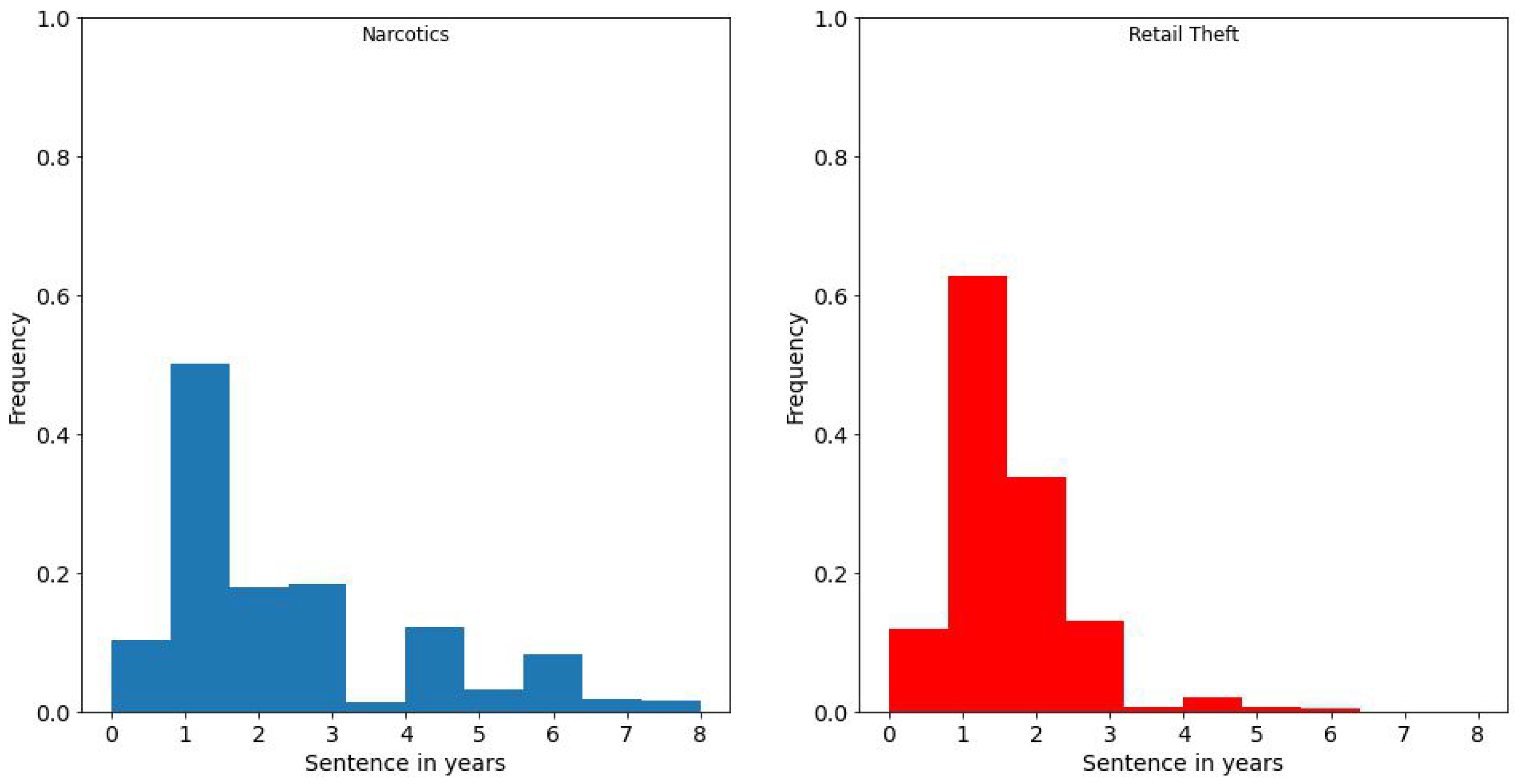
Next, we examine the empirical distribution of sentences shown by (normalized) histograms of sentences for each offense. In Figure 3, we note that the empirical distribution is more concentrated for Retail Theft than for Narcotics. This means that sentencing for retail theft is more consistent across districts than for narcotics.

3. Reason for Decline in Data Point Values

A significant decline in drug offenses and retail theft cases resulting in jail time and probation has been observed in Cooks County due to the implementation of new state laws [9]. These laws prioritize diverting non-violent offenders from the criminal justice system and towards community-based programs and services. As a result, the number of drug and theft cases resulting in jail time and probation has decreased. This shift in approach towards rehabilitation and reintegration has been identified as a contributing factor to the decline in data present for drug- and retail theft-related cases.

4. Constructing Trajectories

To illustrate our approach, we will consider two offenses: narcotics and retail theft. To construct trajectories, we need to cluster sentencing data across all years into k clusters.

We can use any of the clustering methods such as k-means [4]. For simplicity of presentation, in this paper, we consider a simple assignment of sentencing data to $k=4$ patterns based on quartiles $Q_1$, $Q_2$, $Q_3$, and $Q_4$ for each offense. These quartiles are computed from the sentence lengths separately for each offense across ten years (2012–2021). The advantage of such an assignment is that we can compare sentencing patterns for different districts and offenses [3]. Suppose for a particular district $D_i$, and for a particular period, $t_j$, the patterns for both offenses are the same $C_k$. In that case, we can argue that these patterns are similar: both reflect the severity of sentencing according to the quartiles computed for each such offense [10]. By contrast, the sentences themselves cannot be computed directly to each other since they could carry a different severity of punishment depending on the offense.

Let us show how we construct these trajectories. We start with the offense “Narcotics”. For each district and every year we computed the average sentence. This is summarized in

Table 3. Mean annual sentences by district.

YEAR
	1	2	3	4	5	6	7	8	9	10
Narcotics
$D_1$	2.9	3.1	2.8	2.5	2.4	2.5	2.2	2.1	1.7	1.8
$D_2$	1.9	2.2	2.0	1.7	2.6	1.9	1.8	2.2	1.5	1.6
$D_3$	3.5	1.9	3.2	2.9	1.9	2.1	2.1	1.3	2.1	1.9
$D_4$	3.6	5.2	3.7	3.4	3.5	3.8	0.5	0.3	0.5	0.6
$D_5$	1.6	1.9	2.0	2.0	1.9	1.8	1.3	1.8	1.4	1.4
$D_6$	2.9	1.9	2.4	2.7	2.8	2.3	1.1	1.1	0.6	0.6
Retail Theft
$D_1$	1.7	1.7	1.6	1.5	1.4	1.3	1.7	1.3	1.2	1.6
$D_2$	1.6	1.7	1.6	1.6	1.4	1.7	2.3	1.6	1.4	1.6
$D_3$	1.9	1.9	1.7	1.8	1.8	1.9	2.2	1.7	1.4	0.9
$D_4$	1.5	1.9	1.4	1.5	1.2	0.9	0.9	0.8	0.8	0.5
$D_5$	1.7	1.8	1.7	1.5	1.3	1.0	1.5	1.8	2.8	1.2
$D_6$	1.7	1.6	1.5	1.5	1.3	0.9	1.6	1.5	0.7	1.2

:

For Narcotics, the quartiles from the sentencing dataset are $Q_1^{\left(N\right)}=1$, the median $M^{\left(N\right)}=2$, and $Q_3^{\left(N\right)}=3$. If ${\mu }_{ij}^{\left(N\right)}$ is the average sentence for district $D_i$ for year $t_j$, then we consider the following assignment of that district $D_i$ to one of four clusters (patterns): $C_1$, $C_2$, $C_3$, and $C_4$:

1.

$0<{\mu }_{ij}^{\left(N\right)}\le 1$: sentencing pattern $C_1$ (first quartile);

2.

$1<{\mu }_{ij}^{\left(N\right)}\le 2$: sentencing pattern $C_2$ (second quartile);

3.

$2<{\mu }_{ij}^{\left(N\right)}\le 3$: sentencing pattern $C_3$ (third quartile);

4.

$3<{\mu }_{ij}^{\left(N\right)}$: sentencing pattern $C_4$ (fourth quartile).

Once we have the above for assigning patterns, we can construct the corresponding trajectories [11]. For example, take district $D_1$ for Narcotics. We construct its trajectory as follows. From Table 3, for year 1 the mean ${\mu }_{11}^{\left(N\right)}=2.7$ is in the third quartile, and therefore we have sentencing pattern $C_3$. For year 2, the mean ${\mu }_{12}^{\left(N\right)}=2.9$ is in the third quartile, and therefore we again assign sentencing pattern $C_3$. For year 3, the mean ${\mu }_{13}^{\left(N\right)}=3.1$ is in the fourth quartile, and therefore we assign a sentencing pattern $C_4$. Continuing in this manner, we compute the trajectory $P_1^{\left(N\right)}$ of sentencing patterns for the remaining years as $P_1^{\left(N\right)}=(C_3,C_3,C_4,C_3,C_3,C_3,C_3,C_3,C_3,C_2,C_2,C_2)$. In compact notation, we write this as $P_1^{\left(N\right)}=(3,3,4,3,3,3,3,3,3,2,2,2)$. The trajectories for Narcotics are summarized in compact notation in

Table 4. Pattern trajectories by district.

	YEAR
	1	2	3	4	5	6	7	8	9	10	Mode	Count
Narcotics
$D_1$	(3,	4,	3,	3,	3,	3,	3,	3,	2,	2)	$C_3$	7
$D_2$	(2,	3,	3,	2,	3,	2,	2,	3,	2,	2)	$C_2$	6
$D_3$	(4,	2,	4,	3,	2,	3,	3,	2,	3,	2)	$C_2$	4
$D_4$	(4,	4,	4,	4,	4,	4,	1,	1,	1,	1)	$C_4$	6
$D_5$	(2,	2,	3,	3,	2,	2,	2,	2,	2,	2)	$C_2$	8
$D_6$	(3,	2,	3,	3,	3,	3,	2,	2,	1,	1)	$C_3$	5
Retail Theft
$D_1$	(3,	3,	3,	2,	2,	2,	3,	2,	2,	3)	$C_3$	5
$D_2$	(3,	3,	3,	3,	2,	3,	4,	3,	2,	3)	$C_3$	7
$D_3$	(3,	3,	3,	3,	3,	3,	4,	3,	2,	1)	$C_3$	7
$D_4$	(2,	3,	2,	3,	2,	1,	1,	1,	1,	1)	$C_1$	5
$D_5$	(3,	3,	3,	3,	2,	2,	3,	3,	4,	2)	$C_3$	6
$D_6$	(3,	3,	3,	3,	2,	1,	3,	2,	1,	2)	$C_3$	5

.

For retail theft, the quartiles from the sentencing dataset are $Q_1^{\left(R\right)}=1$, the median $M^{\left(R\right)}=1.5$, and $Q_4^{\left(R\right)}=2$. If ${\mu }_{ij}^{\left(R\right)}$ is the average sentence for district $D_i$ for the year j, then we consider the following assignment of that district $D_i$ to clusters (patterns), $C_1$, $C_2$, $C_3$, and $C_4$, like that for Narcotics:

1.

$0<{\mu }_{ij}^{\left(R\right)}\le 1$: sentencing pattern $C_1$ (first quartile);

2.

$1<{\mu }_{ij}^{\left(R\right)}\le 1.5$: sentencing pattern $C_2$ (second quartile);

3.

$1.5<{\mu }_{ij}^{\left(R\right)}\le 2$: sentencing pattern $C_3$ (third quartile);

4.

$2<{\mu }_{ij}^{\left(R\right)}$: sentencing pattern $C_4$ (fourth quartile).

Once we have the above for assigning patterns, we can construct the corresponding trajectories. For example, consider the computation of the trajectory path $P_1^{\left(R\right)}$ for the same district $D_1$. From Table 3, for year 1, the mean ${\mu }_{11}^{\left(R\right)}=1.8$ is in the third quartile and therefore we assign pattern $C_3$. For year 2, the mean ${\mu }_{12}^{\left(R\right)}=1.7$ is in the third quartile, and we assign sentencing pattern $C_3$. For year 3, the mean ${\mu }_{13}^{\left(R\right)}=1.7$ is again in the third quartile, and again we assign a sentencing pattern $C_3$. Continuing in this manner, we compute the trajectory $P_1^{\left(R\right)}$ of sentencing patterns for the remaining years as $P_1^{\left(R\right)}=(C_3,C_3,C_3,C_3,C_2,C_2,C_2,C_3,C_2,C_2,C_3,C_4)$. In compact notation, we write this as $P_1^{\left(R\right)}=(3,3,3,3,2,2,2,3,2,2,3,4)$. The trajectories for retail theft for all districts are summarized in compact notation in Table 4.

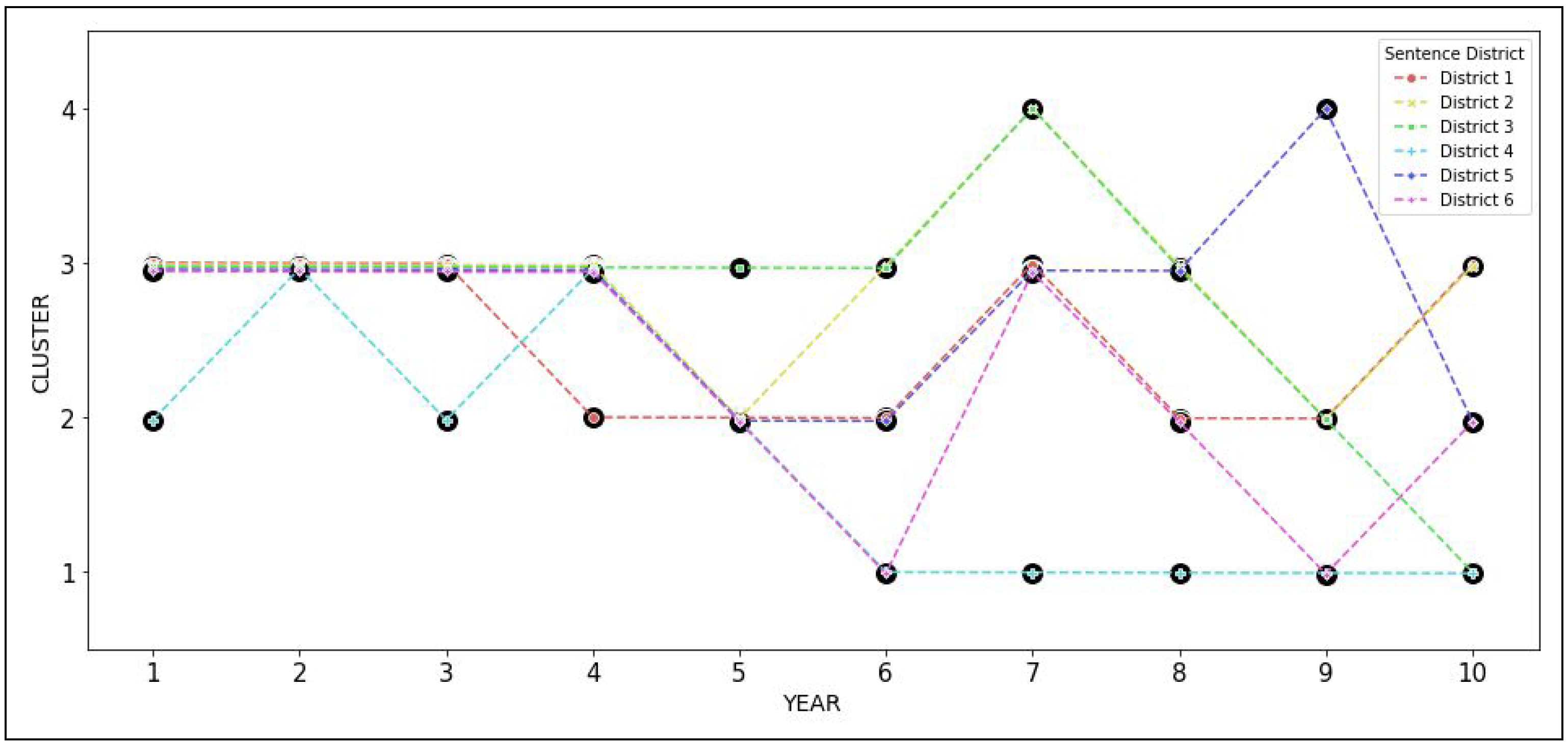
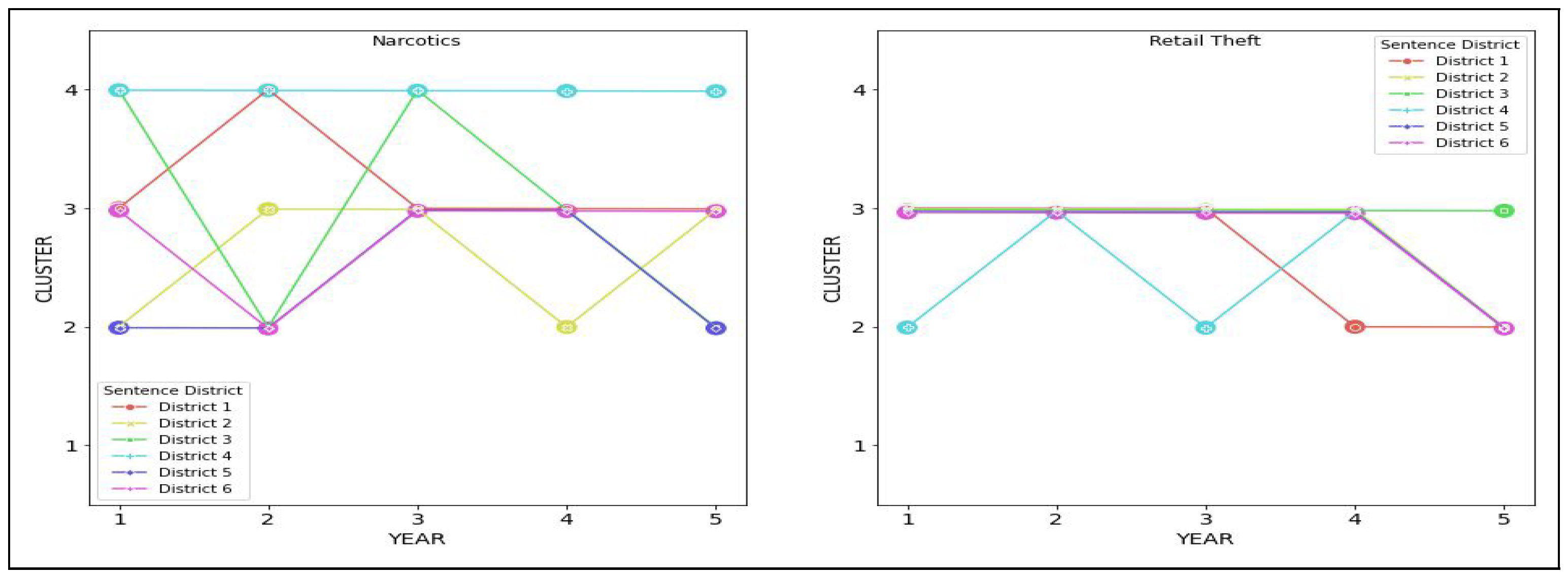
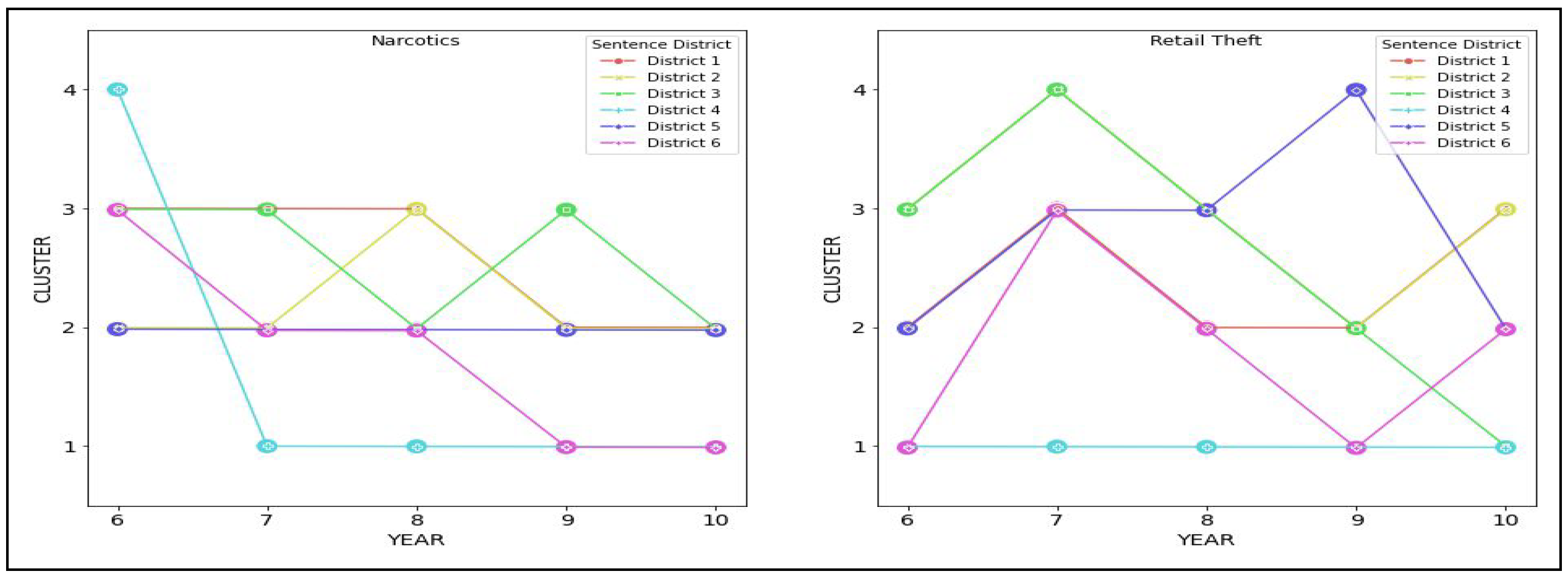
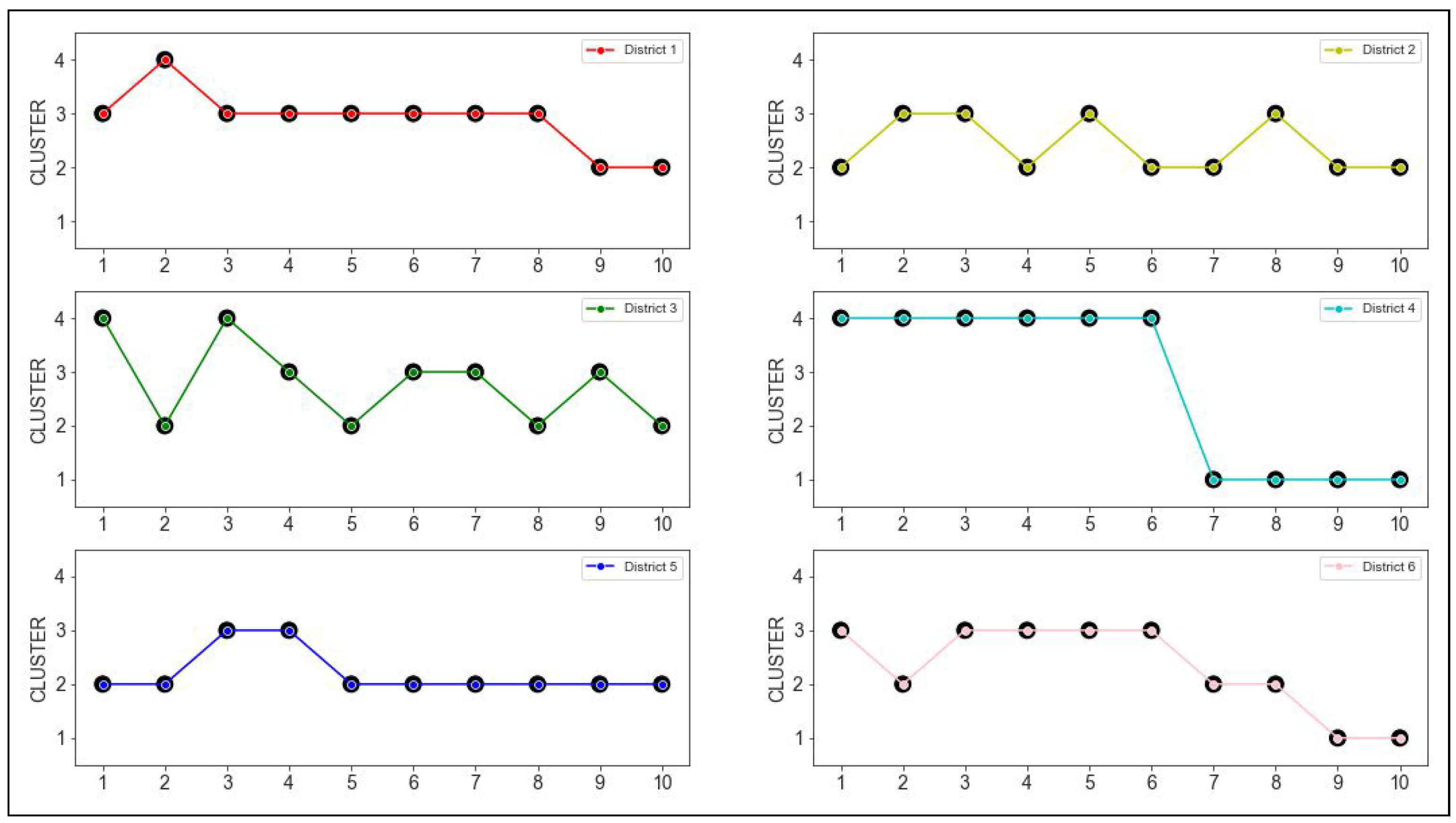
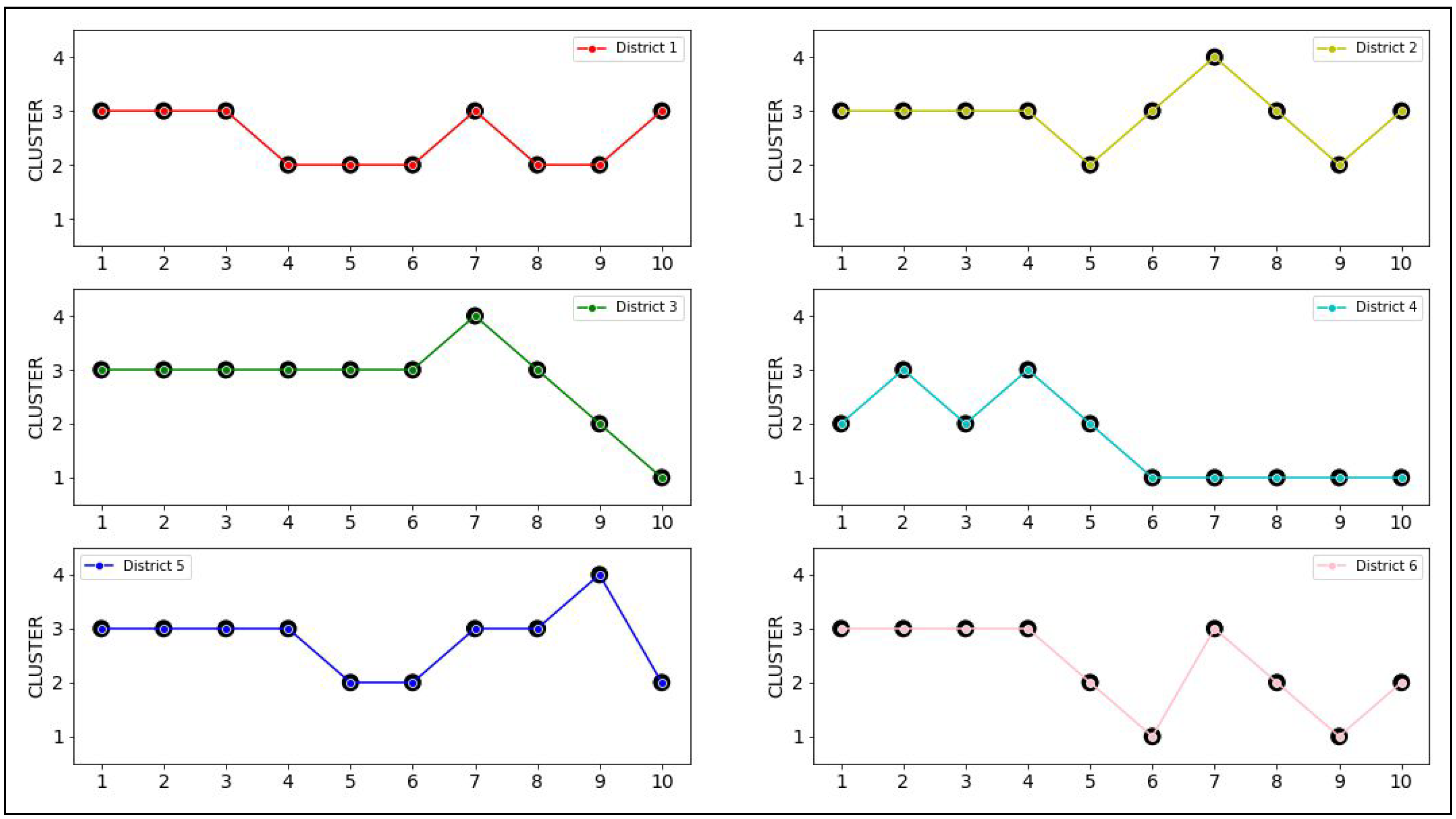
Once we have the assignment of sentencing data to patterns, we can visualize the corresponding trajectories. For Narcotics, the trajectories are shown in Figure 4, and and for retail theft the corresponding trajectories are shown in Figure 5. These trajectories are shown separately for each district in Figure 6 and Figure 7.

Finally, lets us write down the frequency distribution of patterns for each offense. This is summarized in

Table 5. Frequency distribution of patterns.

	Frequency Counts				Percentage
Pattern	$C_1$	$C_2$	$C_3$	$C_4$	$C_1$	$C_2$	$C_3$	$C_4$
Narcotics	6	23	22	9	6%	23%	24%	15%
Retail Theft	8	17	32	3	13%	28%	54%	5%
Narcotics and Retail Theft	14	40	54	12	12%	33%	45%	10%

. For both crimes, more than 80% of patterns are $C_2$ and $C_3$, corresponding to the second and third quartiles in sentence length. It is much more concentrated for Retail Theft: more than 50% of all patterns are pattern $C_3$, whereas, for Narcotics, the number of patterns $C_2$ and $C_3$ are split evenly (38%, 39%). This higher concentration of pattern $C_3$ for Retail Theft reflects a higher percentage of retail theft offenses receiving a higher sentence than narcotics as measured by pattern counts.

5. Analyzing Similarities and Differences

Once the trajectories are computed, we can look for similarity in patterns over time. To that end, we need to define a “distance” metric to measure this.

We propose to use the so-called Hamming distance. In information theory, the Hamming distance between two strings of equal length is the number of positions at which the corresponding symbols are different [12]. If $P_i^{\left(c\right)}$ and $P_j^{\left(c\right)}$ denote two trajectories over n years for some offense c, then the Hamming distance $h(P_i^{\left(c\right)},P_j^{\left(c\right)})$ is defined as the number of years when the corresponding patterns differ. To analyze similarities and differences in sentencing over time, we can analyze the differences between the corresponding trajectories using this Hamming distance [13].

For a simple numerical example, consider the Hamming distance between districts $D_1$ and $D_2$ for Narcotics. The corresponding trajectories are $P_1^{\left(N\right)}$ and $P_2^{\left(N\right)}$ from Table 4:

$$\begin{array}{cc}\hfill \mathrm{Year}& 1,2,3,4,5,6,7,8,9,10\hfill \\ \hfill P_1^{\left(N\right)}& (3,4,3,3,3,3,3,3,2,2)\hfill \\ \hfill & \ne \ne =\ne =\ne \ne ===\hfill \\ \hfill P_2^{\left(N\right)}& (2,3,3,2,3,2,2,3,2,2)\hfill \end{array}$$

There are five years when the corresponding patterns are different. Therefore, for this example, the Hamming distance between trajectories is $h(P_1^{\left(N\right)},P_1^{\left(N\right)})=5$. In other words, for Narcotics, the sentencing patterns for districts $D_1$ and $D_2$ are different in 5 out of 10 years.

In a similar manner, we can compute Hamming distances $h(P_i^{\left(N\right)},P_j^{\left(N\right)})$ for any pair of trajectories from districts $D_i$ and $D_j$. We can summarize these pairwise distances as a hlmatrix ${\mathbf{H}}^{\left(N\right)}$ where an element at row i and column j represents the Hamming distance between trajectory $P_i^{\left(N\right)}$ for district $D_i$ and trajectory $P_j^{\left(R\right)}$ for district $D_j$. Similarly, we can compute the corresponding Hamming matrix ${\mathbf{H}}^{\left(R\right)}$ for trajectories for retail theft.

These corresponding matrices for Narcotics and Retail Theft are given below:

$${\mathbf{H}}^{\left(N\right)}=\left[\begin{array}{cccccc}0& 5& 6& 9& 6& 5\\ 5& 0& 9& 10& 4& 7\\ 6& 9& 0& 8& 5& 6\\ 9& 10& 8& 0& 10& 8\\ 6& 4& 5& 10& 0& 5\\ 5& 7& 6& 8& 5& 0\end{array}\right],{\mathbf{H}}^{\left(R\right)}=\left[\begin{array}{cccccc}0& 4& 6& 8& 4& 4\\ 4& 0& 2& 7& 4& 5\\ 6& 2& 0& 7& 5& 6\\ 8& 7& 7& 0& 7& 5\\ 4& 4& 5& 7& 0& 3\\ 4& 5& 6& 5& 3& 0\end{array}\right]$$

We note that each Hamming matrix is symmetric with 0 on the main diagonal. For $n=6$ districts, each matrix contains $(n^2-n)/2=15$ entries (Hamming distances) above the main diagonal corresponding to distinct pairs of trajectories. Let us write down these 15 entries as sorted sequences for Narcotics and Retail Theft. We will denote these sequences as $S^{\left(N\right)}$ and $S^{\left(R\right)},$ respectively. We have the following:

$$\begin{array}{cc}\hfill S^{\left(N\right)}& =\{4,5,5,5,5,6,6,6,7,8,8,9,9,10,10\}\hfill \\ \hfill S^{\left(R\right)}& =\{2,3,4,4,4,4,5,5,5,6,6,7,7,7,8\}\hfill \end{array}$$

We can compute some statistical measures for each of these two sequences and summarize them in

Table 6. Statistics of Hamming distances for Narcotics and Retail Theft.

Sequence	Min	Max	Mode	Median	$\mathit{\mu }$	$\mathit{\sigma }$
$S^{\left(N\right)}$	4	10	5	6	6.9	1.9
$S^{\left(R\right)}$	4	8	4	5	5.1	1.6

. This table shows that both median and mean Hamming distances are lower for Retail Theft than for Narcotics. On average, the two trajectories differ in almost seven out of ten years (or 70% of the time) for Narcotics ($\mu =6.9$) but only in about five years out of ten years (or 50%) for Retail Theft ($\mu =5.1$). The variability in these distances measured by standard deviations is lower for Retail Theft ($\sigma =1.6$) than for Narcotics ($\sigma =1.9$). In other words, retail theft sentencing was comparatively more consistent across districts than narcotics sentencing.

6. Volatility and Inertia of a Trajectory

In the previous section, we examined the similarities between trajectories using the Hamming distance. We now focus on describing the statistics on individual trajectories. We want to characterize the following performance metrics:

1.

The tendency of a trajectory to change patterns over time. We will call this the volatility of trajectory and denote it by V.

2.

The tendency of a trajectory to remain in the same pattern in consecutive years. We will call the length of the longest such sub-sequence the inertia of the trajectory. We denote inertia by I.

3.

The “average” or “most likely” trajectories for Narcotics and Retail Theft.

We start with volatility. Suppose a pattern in each period was described by a single number. In that case, we could take some measure of deviation, such as standard deviation, and use it as a measure of volatility [14]. However, in general, we may not have such a single numerical description of a pattern. Therefore, we suggest a simple alternative: measure trajectory volatility by the number of times patterns were switched in the trajectory [15].

For example, consider district $D_1$ for Narcotics. Its trajectory is

$$\begin{array}{cc}\hfill \mathrm{Year}& 12345678910\hfill \\ \hfill P_1^{\left(N\right)}& (3,4,3,3,3,3,3,3,2,2)\hfill \end{array}$$

This trajectory switched patterns after years 2, 3, 4, and 9. We can write it schematically as

$$P_1^{\left(N\right)}=(3\nearrow 4\searrow 3,3,3,3,3,3\searrow 2,2)$$

where ↗ and ↘ represent changes to a higher-numbered pattern or a lower-numbered pattern, respectively. Therefore, the above trajectory $P_1^{\left(N\right)}$ had three switches between patterns. We use this number as a measure of volatility for trajectories. Therefore, $V\left(P_1^{\left(N\right)}\right)=3$.

We compute this volatility $V^{\left(R\right)}$ and $V^{\left(R\right)}$ for the Narcotics and Retail Theft trajectories, respectively, and summarize the results in

Table 7. Volatility and inertia of trajectories.

${\mathit{D}}_{\mathit{i}}$	Trajectory Switching Pattern	V	I
Narcotics
$D_1$	3 ↗ 4 ↘ (3, 3, 3, 3, 3, 3) ↘ (2, 2)	3	6
$D_2$	2 ↗ (3, 3) ↘ 2 ↗ 3 ↘ (2, 2) ↗ 3 ↘ (2, 2)	6	2
$D_3$	4 ↘ 2 ↗ 4 ↘ 3 ↘ 2 ↗ (3, 3)↘ 2 ↗ 3 ↘ 2	8	2
$D_4$	(4, 4, 4, 4, 4, 4) ↘ (1, 1, 1, 1)	1	6
$D_5$	(2, 2) ↗ (3, 3) ↘ (2, 2, 2, 2, 2, 2)	2	6
$D_6$	3 ↘ 2 ↗ (3, 3, 3, 3) ↘ (2, 2) ↘ (1, 1)	4	4
$\mu :$		3.0	4.3
$\sigma :$		2.6	2.0
Retail Theft
$D_1$	(3, 3, 3) ↘ (2, 2, 2) ↗ 3 ↘ (2, 2) ↗ 3	4	3
$D_2$	(3, 3, 3, 3) ↘ 2 ↗ 3 ↗ 4 ↘ 3 ↘ 2 ↗ 3	6	4
$D_3$	(3, 3, 3, 3, 3, 3) ↗ 4 ↘ 3 ↘ 2 ↘ 1	4	6
$D_4$	2 ↗ 3 ↘ 2 ↗ 3 ↘ 2 ↘ (1, 1, 1, 1, 1)	5	5
$D_5$	(3, 3, 3, 3) ↘ (2, 2) ↗ (3, 3) ↗ 4 ↘ 2	4	4
$D_6$	(3, 3, 3, 3) ↘ 2 ↘ 1 ↗ 3 ↘ 2 ↘ 1 ↗ 2	6	4
$\mu :$		4.8	4.3
$\sigma :$		1.0	1.0

. From this table, we see that for Retail Theft, we have a slightly higher mean volatility (5.3 vs. 4.7) but a lower standard deviation (0.9 vs. 2.1). Examining the pattern of switches, we notice that for Retail Theft, there are many more switches in the last 6 years compared to Narcotics. This suggests that sentencing patterns in the last six years could be quite different than in the first six years. We will present a detailed analysis of such comparison in Section 7.

Next, we consider inertia—the tendency of a trajectory to stay in the same pattern over consecutive years. We analyze inertia by computing the length of the longest sub-sequence with the same pattern.

For example, consider district $D_1$ for Narcotics. Its trajectory is

$$\begin{array}{cccccccccc}\mathrm{Year}& 1& 2& 3& 4& 5& 6& 7& 8& 910\\ P_1^{\left(N\right)}& (3,& 4,& (3,& 3,& 3,& 3,& 3,& 3),& 2,2)\end{array}$$

This trajectory spends 6 consecutive years in the same pattern $C_3$. It is possible to have a case where we have multiple sub-sequences with the same duration. In such a case, we take the length of a maximum sub-sequence. For example, consider district $D_3$

$$\begin{array}{cccccccccc}\mathrm{Year}& 1& 2& 3& 4& 5& 6& 7& 8& 910\\ P_2^{\left(N\right)}& (2,& (3,& 3),& 2,& 3,& (2,& 2),& 3,& (2,2))\end{array}$$

In this example, we have three sub-sequences of the same length, 2. In such a case, we will use a sub-sequence containing the most frequent pattern. For this district, pattern $C_2$ is the most frequent and, therefore, we will use $(2,2)$ as the sub-sequence to measure inertia.

In Table 7, we present the results for inertia for both offenses. The average inertia is slightly higher for Retail Theft vs. Narcotics (5.3 vs. 4.7) and has a lower standard deviation (0.9 vs. 1.8). This suggests that sentencing patterns for retail theft are more static.

Finally, we can ask the following question: what are the “average” or most likely trajectories for Narcotics and Retail Theft? [16] We can construct such trajectories as follows. For each offense and year, we write down the most frequent (mode) pattern for that year. This is illustrated in

Table 8. Computing “average” trajectories.

YEAR
	1	2	3	4	5	6	7	8	9	10
Narcotics	{2,3,4}	2	3	3	3	3	2	2	2	2
Retail Theft	3	3	3	3	2	{1,2,3}	3	3	2	{1,2,3}

.

For some years, we may have multiple choices for the mode. For example, for Narcotics, we have multiple choices for year 1, namely clusters $C_2$, $C_3$, and $C_4$. For Retail Theft, we have multiple choices for year 6 (clusters $C_1$, $C_2$, and $C_3$) and year 10 (clusters $C_1$, $C_2$, and $C_3$). In such cases, we will use the procedure commonly used in machine learning [1,4]: use the most frequent pattern across all districts and years for that offense. For example, for year 1 in Narcotics, we must choose between patterns $C_2$ and $C_3$. From Table 5, we find that for Narcotics, pattern $C_2$ is (slightly) more frequent than pattern $C_3$ (23% vs. 22%). Therefore, we assign $C_2$ for year 2 in Narcotics.

By contrast, for Retail Theft from Table 5, we find that pattern $C_3$ is much more frequent than $C_2$ (54% vs. 28%). Therefore, we assign pattern $C_3$ in years 6 and 10.

With the above construction, we can compute the “average” trajectories, their volatility V, and inertia I for Narcotics and Retail Theft:

$$\begin{array}{cccccccccc}\mathrm{Year}& 1& 2& 3& 4& 5& 6& 7& 8& 910\\ P_{ave}^{\left(N\right)}& (2,& 2,& 3,& 3,& 3,& 3,& (2,& 2,& 2,2\left)\right)\\ P_{ave}^{\left(R\right)}& \left(\right(3,& 3,& 3,& 3),& 2,& 3,& 3,& 3,& 2,3)\end{array}$$

Let us rewrite the above paths by indicating pattern switches and sub-trajectories in the same cluster.

$$\begin{array}{cc}\hfill P_{ave}^{\left(N\right)}& =\left(\right(2,2)\nearrow (3,3,3,3)\searrow (2,2,2,2\left)\right)\hfill \\ \hfill P_{ave}^{\left(R\right)}& =\left(\right(3,3,3,3)\searrow 2\nearrow (3,3,3)\searrow 2\nearrow 3)\hfill \end{array}$$

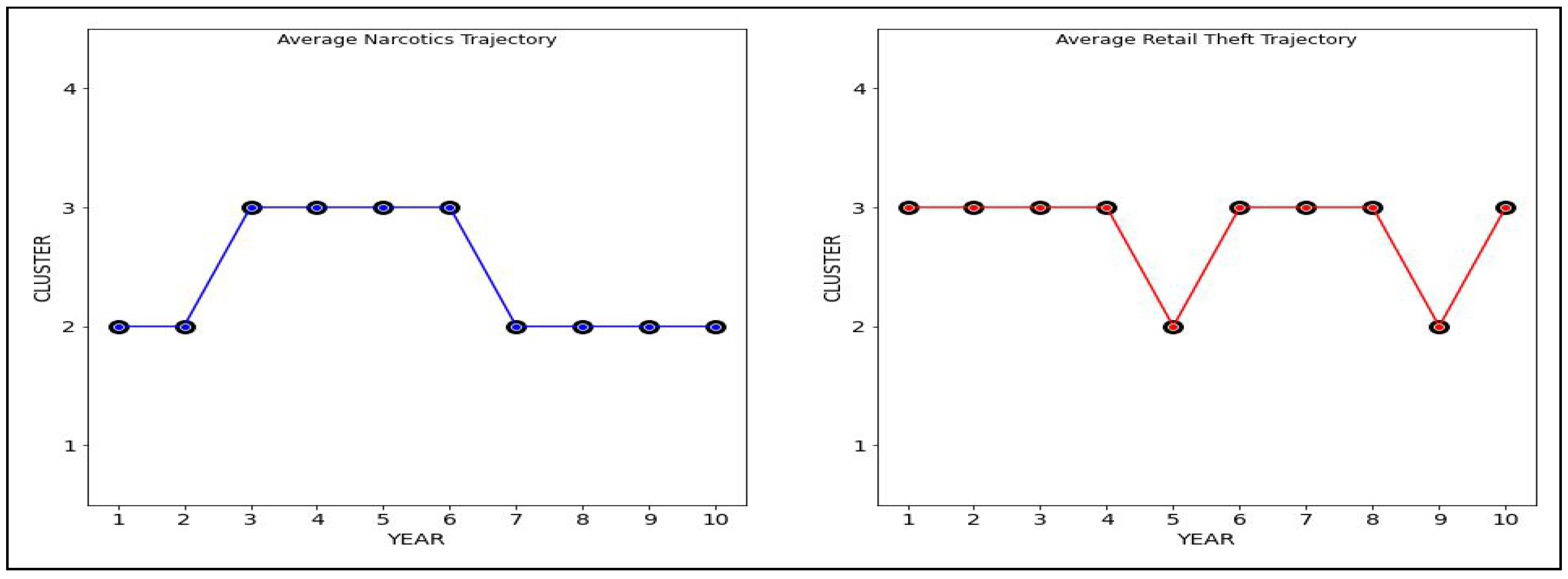
These “average” trajectories are illustrated in Figure 8. Comparing these new “average” trajectories, we note the following:

1.

For Narcotics, the trajectory has inertia $I=5$. It spends the last five years in pattern $C_2$. During the first 7 years, it switched between patterns $C_2$ and $C_3$. Its volatility is $V=3$.

2.

For Retail Theft, the trajectory also has inertia $I=5$, but it spends the first five years in pattern $C_3$. During the last seven years, it has switched between patterns $C_2$ and $C_3$. Its volatility is $V=5$ and is higher than that of Narcotics.

7. Changes in Sentencing Patterns over Aggregated Time Periods

In the previous analysis, we constructed the trajectory for patterns and analyzed their similarity and differences by focusing on all 10 years. We now ask the following question: do differences in patterns change over larger (aggregated) periods [17]?

We illustrate how such analysis is carried out with our trajectories. We will aggregate our ten years into the first five years (years 1–5) and the last five years (years 6–10). Consider the Narcotics offenses first. If we take district $D_i$, then its trajectory $P_1^{\left(N\right)}$ from Table 4,

$$P_1^{\left(N\right)}=(3,4,3,3,3,3,3,3,2,2),$$

will be split into sub-trajectories $F_1^{\left(N\right)}$ and $L_1^{\left(N\right)}$ corresponding to the first five and last five years, respectively,

$$F_1^{\left(N\right)}=(3,4,3,3,3),L_1^{\left(N\right)}=(2,3,4,3,3).$$

We can split all trajectories into two halves. The resulting partial trajectories are summarized in

Table 9. Sub-trajectories for years 1–6 and years 7–12.

	Narcotics		Retail Theft
	Years 1–5	Years 6–10	Years 1–5	Years 6–10
	${\mathit{F}}_{\mathit{i}}^{\left(\mathit{N}\right)}$	${\mathit{L}}_{\mathit{i}}^{\left(\mathit{N}\right)}$	${\mathit{F}}_{\mathit{i}}^{\left(\mathit{R}\right)}$	${\mathit{F}}_{\mathit{i}}^{\left(\mathit{R}\right)}$
$D_1$	$(3,4,3,3,3)$	$(3,3,3,2,2)$	$(3,3,3,2,2)$	$(2,3,2,2,3)$
$D_2$	$(2,3,3,2,3)$	$(2,2,3,2,2)$	$(3,3,3,3,2)$	$(3,4,3,2,3)$
$D_3$	$(4,2,4,3,2)$	$(3,3,2,3,2)$	$(3,3,3,3,3)$	$(3,4,3,2,1)$
$D_4$	$(4,4,4,4,4)$	$(4,1,1,1,1)$	$(2,3,2,3,2)$	$(1,1,1,1,1)$
$D_5$	$(2,2,3,3,2)$	$(2,2,2,2,2)$	$(3,3,3,3,2)$	$(2,3,3,4,2)$
$D_6$	$(3,2,3,3,3)$	$(3,2,2,1,1)$	$(3,3,3,3,2)$	$(1,3,2,1,2)$

.

The trajectories are illustrated in Figure 9 and Figure 10:

Once we have the sub-trajectories, we can compute the Hamming matrices for the first and last five years. We will use the subscripts $\left(f\right)$ and $\left(l\right)$ to denote the first five years and the last five years. With this notation, we have the following:

1.

Hamming distance matrices for Narcotics in the first and last five years:

$${\mathbf{H}}_f^{\left(N\right)}=\left[\begin{array}{cccccc}0& 3& 4& 4& 3& 1\\ 3& 0& 5& 5& 3& 3\\ 4& 5& 0& 3& 2& 3\\ 4& 5& 3& 0& 5& 5\\ 3& 3& 2& 5& 0& 2\\ 1& 3& 3& 5& 2& 0\end{array}\right],{\mathbf{H}}_l^{\left(N\right)}=\left[\begin{array}{cccccc}0& 2& 2& 5& 3& 4\\ 2& 0& 4& 5& 1& 4\\ 2& 4& 0& 5& 3& 3\\ 5& 5& 5& 0& 5& 3\\ 3& 1& 3& 5& 0& 3\\ 4& 4& 3& 3& 3& 0\end{array}\right]$$

2.

Hamming distance matrices for first and last five years for Retail Theft:

$${\mathbf{H}}_f^{\left(R\right)}=\left[\begin{array}{cccccc}0& 1& 2& 3& 1& 1\\ 1& 0& 1& 2& 0& 0\\ 2& 1& 0& 3& 1& 1\\ 3& 2& 3& 0& 2& 2\\ 1& 0& 1& 2& 0& 0\\ 1& 0& 1& 2& 0& 0\end{array}\right],{\mathbf{H}}_l^{\left(R\right)}=\left[\begin{array}{cccccc}0& 3& 4& 5& 3& 3\\ 3& 0& 1& 5& 4& 5\\ 4& 1& 0& 4& 4& 5\\ 5& 5& 4& 0& 5& 3\\ 3& 4& 4& 5& 0& 3\\ 3& 5& 5& 3& 3& 0\end{array}\right]$$

As before, for our $n=6$ districts, each Hamming distance matrix contains $(n^2-n)/2=15$ entries (Hamming distances for sub-trajectories). We can write down these entries in sorted order. As with the Hamming matrices above, we will use subscripts $\left(f\right)$ and $\left(g\right)$. We have

$$\begin{array}{cc}\hfill S_f^{\left(N\right)}& =\{1,2,2,3,3,3,3,3,3,4,4,5,5,5,5\}\hfill \\ \hfill S_l^{\left(N\right)}& =\{1,2,2,3,3,3,3,3,4,4,4,5,5,5,5\}\hfill \\ \hfill S_f^{\left(R\right)}& =\{0,0,0,1,1,1,1,1,1,2,2,2,2,3,3\}\hfill \\ \hfill S_l^{\left(R\right)}& =\{1,3,3,3,3,3,4,4,4,4,5,5,5,5,5\}\hfill \end{array}$$

As before, we can compute some statistical measures for Hamming distances for each sequence. These are summarized in

Table 10. Statistics of Hamming distances for Narcotics and Retail Theft in the first and last five years.

Offense	Years	Min	Max	Median	$\mathit{\mu }$	$\mathit{\sigma }$
Narcotics	1–5	1	5	3	3.4	1.2
	6–10	1	5	3	3.5	1.2
Retail Theft	1–5	0	3	1	1.3	0.9
	6–10	1	5	4	3.8	1.1

. We note that for Narcotics, the statistics on Hamming distances have remained practically unchanged between the two periods. The median Hamming distance for Narcotics remained the same, and the mean changed slightly between the first five years ($\mu =3.4$) and the last five years ($\mu =3.5$). The standard deviation remained the same at $\sigma =1.2$.

By contrast, we see a dramatic difference between the first and last periods for Retail Theft. In the first period, the sub-trajectories were very similar, with a median Hamming distance of 1. This median distance increased dramatically to 4 in the second period. The mean distance increased dramatically from 1.3 to 3.8. At the same time, the variability in Hamming distances increased only slightly from $\sigma =0.9$ to $\sigma =1.1$. In other words, the sub-trajectories for Retail Theft became considerably more distinct in the last five years than during the first five years.

Next, we compare both periods separately in terms of volatility V and inertia I. We compute these by examining Table 9. Our results are summarized in

Table 11. Volatility V and inertia I for sub-trajectories.

	Narcotics				Retail Theft
	Years 1–5		Years 6–10		Years 1–5		Years 6–10
	$\mathit{I}$	$\mathit{V}$	$\mathit{I}$	$\mathit{V}$	$\mathit{I}$	$\mathit{V}$	$\mathit{I}$	$\mathit{V}$
$D_1$	3	2	3	1	3	1	2	3
$D_2$	2	3	2	2	4	1	1	4
$D_3$	1	4	2	3	5	0	1	4
$D_4$	5	0	4	1	1	4	5	0
$D_5$	2	2	5	0	4	1	2	3
$D_6$	3	2	2	2	4	1	1	4
$\mu$	2.7	2.2	3.0	1.5	3.5	1.3	2.0	3.0
$\sigma$	1.4	1.3	1.3	1.0	1.4	1.4	1.5	1.5

. Examining this table, we see a dramatic change in sentencing between the two periods. For Narcotics, the average inertia $\mu \left(I\right)$ increased from 2.7 to 3, while the average volatility $\mu \left(V\right)$ decreased from 2.2 to 1.5. The standard deviations for both inertia and volatility decreased as well. By contrast, for Retail Theft, the average inertia $\mu \left(I\right)$ decreased drastically from $3.5$ to 2, while the average volatility $\mu \left(V\right)$ increased drastically from 1.3 to 3. Standard deviations for these measures increased, especially for volatility from 1.3 to 3. This means that for Retail Theft, the districts became much more different in their sentencing patterns. The most dramatic change for Retail Theft is observed in district $D_3$. For the first five years, the trajectory remained in the same cluster $C_3$, whereas it changed clusters from one year to the next for the last five years. These results are consistent with the above observation that sub-trajectories became more distinct for Retail Theft than for Narcotics when measured by Hamming distances.

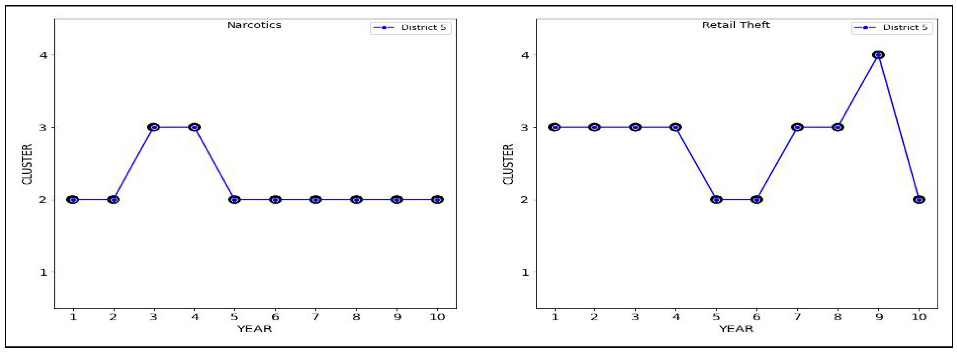
8. Side-by-Side Comparison of Districts

So far, we have compared trajectories to each other separately for Narcotics and Retail Theft and have identified differences and similarities in sentencing patterns. We now ask a different question: how do individual districts compare in terms of their sentencing patterns [18]?

We can only make such a comparison if we have the same number of patterns and each cluster $C_i$ for Narcotics is “equivalent” to cluster $C_i$ for Retail Theft. In our case, we took the same number $k=4$ of clusters, and districts were assigned to clusters by similar rules based on quartiles of average sentences. Therefore, although the sentences could be radically different, we can compare the individual districts in corresponding patterns. Side-by-side comparisons are shown in Figure 11 and Figure 12.

In

Table 12. Side-by-side comparison of districts.

		YEAR
${\mathit{D}}_{\mathit{i}}$	$\left(\mathit{c}\right)$	1	2	3	4	5	6	7	8	9	10	$\mathit{V}$	$\mathit{I}$	$\mathit{h}$
$D_1$	(N)	3	4	3	3	3	3	3	3	2	2	2	6	6
	(R)	3	3	3	2	2	2	3	2	2	3	4	3
$D_2$	(N)	2	3	3	2	3	2	2	3	2	2	7	3	6
	(R)	3	3	3	3	2	3	4	3	2	3	6	4
$D_3$	(N)	4	2	4	3	2	3	3	2	3	2	8	2	8
	(R)	3	3	3	3	3	3	4	3	2	1	4	6
$D_4$	(N)	4	4	4	4	4	4	1	1	1	1	2	6	6
	(R)	2	3	2	3	2	1	1	1	1	1	5	5
$D_5$	(N)	2	2	3	3	2	2	2	2	2	2	2	6	5
	(R)	3	3	3	3	2	2	3	3	4	2	4	4
$D_6$	(N)	3	2	3	3	3	3	2	2	1	1	4	4	5
	(R)	3	3	3	3	2	1	3	2	1	2	6	4

, we consider pairwise trajectories for each district and compute their volatility V and inertia I from Table 7 and their Hamming distances $h(P_i^{\left(N\right)},P_i^{\left(R\right)})$.

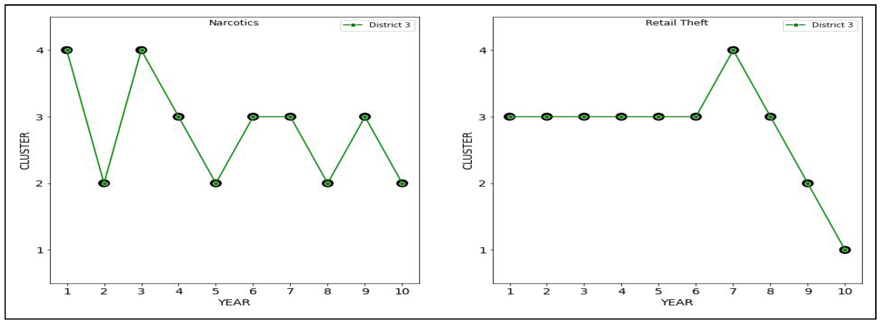
We can see that the most significant difference is in district $D_3$.

For this district, the Hamming distance is 8. For Narcotics, this district has a maximum value of 8 for volatility and a minimum value of 2 for inertia across all possible trajectories. By contrast, for Retail Theft, this district has a median volatility value of 4 but a maximum value of 6 for inertia across all possible trajectories.

The most minor difference is in district $D_5$, with a Hamming distance of 6.

For both Narcotics and Retail Theft, we have the same value of 7. For Narcotics, this district has a value of 3. By contrast, for Retail Theft, this district has an inertia value of 4, which is the median value for inertia across all trajectories.

The above comparison suggests that district 3 has the most differences in sentencing patterns for both offenses, whereas district 5 has the most similar patterns in sentencing.

9. Summary of Results and Discussion

Let us start by summarizing our findings for Narcotics and Retail Theft.

• The median and mean Hamming distances are lower for Retail Theft than for Narcotics, suggesting that retail theft sentencing was more consistent than Narcotics sentencing
• The volatility of trajectories was much higher for Retail Theft than for Narcotics
• the inertia is similar for both Narcotics and Retail Theft
• For Narcotics, the sentencing patterns did not change much during the last five years as compared to the first five years. For Retail Theft, there was a dramatic change in sentencing patterns as measured by changes in Hamming distances, inertia, and volatility
• In a side-by-side comparison of sentencing by district, the most consistent sentencing for both offenses was carried out by district 2, and the most inconsistent sentencing was carried out by district 3

10. Conclusions

In this paper, we presented a general approach to compare sentencing data. The key idea is to associate sentencing data with a small number of patterns (clusters) for each period. This allows a representation of (possibly multi-dimensional) sentencing data in terms of trajectories in the (time, cluster) space. We defined inertia and volatility for these trajectories and used Hamming distance to analyze similarities and differences in sentencing based on visualization. We illustrated our approach by presenting a detailed comparison of sentencing data for Narcotics and Retail Theft. We believe the proposed approach would provide additional tools for quantitative analysis in criminology.