1. Introduction
Project planners are faced with a great challenge in determining the number of resources to use on a construction project. Hence, effective planning of construction projects is vital to achieve the project objectives. Failing to select the optimal combination of equipment, crews, and project settings can result in prolonged project durations and an unnecessary cost overrun. Stochastic simulation optimization, which is the combination of stochastic simulation with optimization algorithms, has been proposed by several researchers to optimize construction operations [
1,
2,
3]. Explicit averaging (EA) is the de facto method of estimating objective functions when stochastic simulation is used [
4]. This is done by calculating the average value of the objective functions obtained from a number of simulation replications. Traditional stochastic simulation optimization frameworks are limited by the long computation time required to solve the optimization problem and the large number of simulation replications required to obtain an accurate estimate of the objective functions [
5]. In the field of construction management, previous work used parallel computing [
6], variance reduction techniques [
7], and the joint application of the previous two approaches [
5] to overcome these limitations.
The main objective of this paper is to study the benefits of applying (1) implicit averaging (IA) and (2) implicit averaging with common random numbers (ICRN) in construction simulation optimization problems. Implicit averaging refers to using a single simulation replication to estimate the objective functions. Common Random Numbers (CRN) is a variance reduction technique that is used to compare the performance of a simulation model across different candidate solutions [
8]. The concept of CRN is that the decision-maker wants to compare the performance of the different candidate solutions under the same uncertainty conditions so that any improvement in the performance is solely due to the change in the resource combination. The anticipated benefits of using IA and ICRN are (1) a reduction in the computation time, (2) an improvement in the quality of optimum solutions, and (3) an increase in the number of evaluated candidate solutions. The rest of the paper is organized as follows:
Section 2 presents the methods used in this study,
Section 3 presents the results and discussion, and
Section 4 provides conclusions and future work.
2. Methods
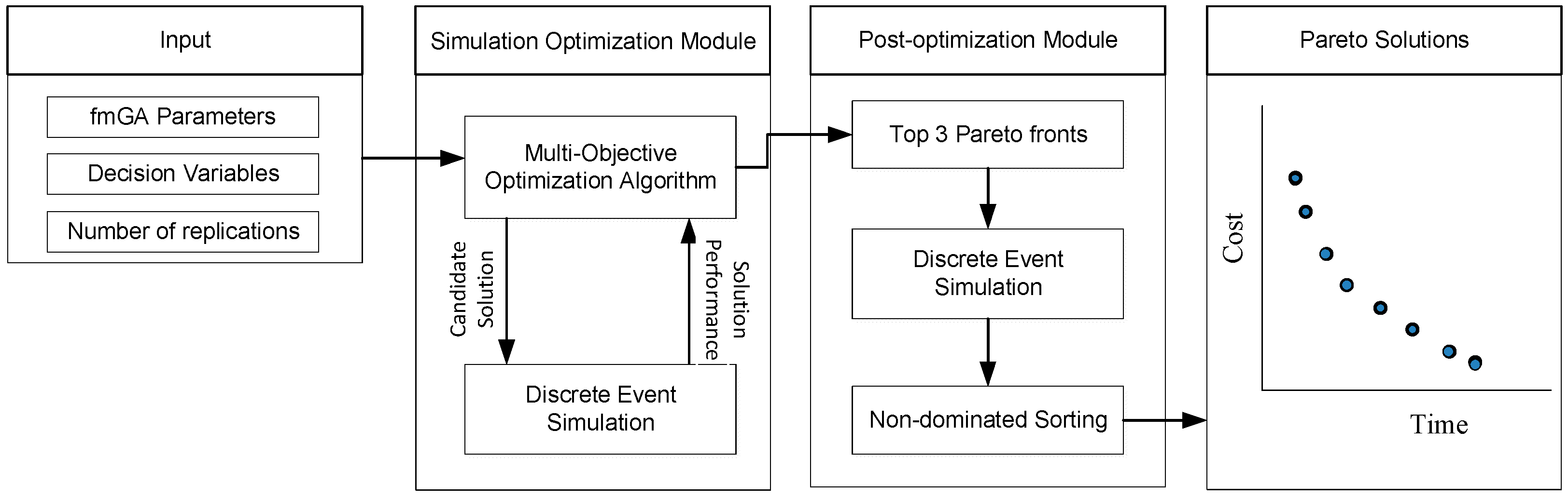
This section presents the proposed simulation optimization framework that can be used by project planners to enhance decision-making on construction projects. The aim of the proposed framework is to obtain near-optimum recourse combinations that minimize the duration and cost of a construction project. It consists of the simulation optimization and post-optimization analysis modules, as shown in
Figure 1.
The simulation optimization module integrates a multi-objective optimization algorithm and discrete event simulation to obtain a set of Pareto fronts. The fast messy Genetic Algorithm (fmGA) [
9] is used to search the space of the decision variables and generate candidate solutions by combining these decision variables. It is worth mentioning that other optimization algorithms can be used in place of fmGA. This module uses IA and ICRN when evaluating the generated candidate solutions. Discrete event simulation is used to estimate the objective functions (i.e., duration and cost) of candidate solutions. These estimates are used by fmGA to guide its search for near-optimum solutions. The output of this module is a set of Pareto fronts, which is the preferable outcome of a multi-objective optimization problem. These Pareto solutions are non-dominated optimum solutions that represent the potential tradeoff among the project objectives.
An important criterion for the success of the CRN is the synchronization of the random numbers. In this paper, CRN are implemented for each stochastic task in the simulation model. To maintain appropriate synchronization among these stochastic tasks, each task is allocated a separate stream from which random numbers can be generated. Algorithm 1 shows the summary of the algorithm for the simulation optimization module. The process starts by generating and storing a random seed number. This stored seed number is used across all the candidate solutions for proper synchronization and dependency between them. The fmGA would then generate the initial population. Each generated population would go through the same steps of evaluating the candidate solutions using stochastic simulation, sorting the population, and applying genetic operators to generate a new population until the termination criterion is met. At that point, the fmGA would return the top three ranks of Pareto solutions.
The purpose of the second module is to take a deeper look into the top three Pareto fronts that are obtained from the first module. The reasoning behind that is to ensure that no non-dominated solutions are left behind in the Pareto fronts of rank 2 and 3. Each solution in the top three ranks is evaluated using a large number of replications (i.e., 1000) to obtain sound statistical information on these solutions. Finally, non-dominated sorting is performed on these solutions to filter out inferior solutions and present the final Pareto solutions.
| Algorithm 1 Summary of simulation optimization module |
| 1: | Generate and store seed number |
| 2: | Initialize population |
| 3: | FOR each generation until termination DO |
| 4: | FOR each solution in a population |
| 5: | Run simulation |
| 6: | Generate streams using seed number |
| 7: | Calculate duration and cost |
| 8: | Sort population and apply genetic operators |
| 9: | RETURN Pareto fronts of ranks 1, 2, and 3 |
2.1. Performance Metrics
Three performance metrics are used to measure the performance of the presented framework. The first metric is the achieved time savings, as shown in Equation (1). It measures the reduction in computation time of the optimization process that is realized by using IA or ICRN.
where
Ts is the achieved time savings, and
TEA and
TPF are the time required to solve the optimization problem using EA and the presented framework, respectively.
The second metric is the change in the hypervolume indicator, as shown in Equation (2). This metric is used to compare the performance of multi-objective evolutionary algorithms [
10]. Using this indicator, the area of the search space dominated by the Pareto front is calculated [
11]. When comparing multiple Pareto fronts, the one with the largest area (i.e., hypervolume indicator) is the superior Pareto front, since it considers the front’s optimality and diversity [
12].
where ∆
HV is the percentage difference in the hypervolume indicator,
HVEA is the hypervolume indicator using EA, and
HVPF is the hypervolume indicator using the proposed framework.
The third metric is the change in the number of evaluated candidate solutions over a finite period of time. This metric can be used to measure the confidence level in the optimality of the Pareto solutions.
where ∆
ES is the percentage difference in the number of evaluated candidate solutions, and
ESEA and
ESPF are the number of evaluated candidate solutions representing EA and the proposed framework.
2.2. Implementation
The simulation optimization module is implemented by embedding STROBOSCOPE simulation software [
13] within the Darwin optimization framework [
14], which utilizes fmGA, as shown in
Figure 2. The integration of these two tools is done in Microsoft Visual C#. The minimum, maximum, and increment values for each decision variable is stored in a text file. The optimization tool accesses the text file and generates the candidate solutions using the specified boundaries. The developed code would then modify values of the decision variables within the simulation source code. Then, it starts the simulation tool and creates a new model with the modified source code. Next, it runs the simulation and extracts the project duration and cost. Finally, the code exports the project duration and cost to the optimization tool. At the termination of the optimization, the Pareto solutions are output into a text file.
To perform the post-optimization analysis, Microsoft Excel via VBA is used to re-evaluate the Pareto solutions. This is done in a similar manner as in the simulation optimization module. Once the re-evaluation is completed, a non-dominated sorting is performed to present the final Pareto front.
3. Results and Discussion
The study used in this paper consists in constructing a precast box girder bridge using a full-span launching gantry method. The developed simulation model and study details can be found in [
5]. The bridge consists of 35 spans with identical spans measuring a length of 25 m. This construction method has the following three phases: (1) casting the spans at the casting yard, (2) delivering the spans to the construction site, and (3) erecting the spans. The study considers 13 decision variables related to the settings of the casting yard and the transportation of box girders.
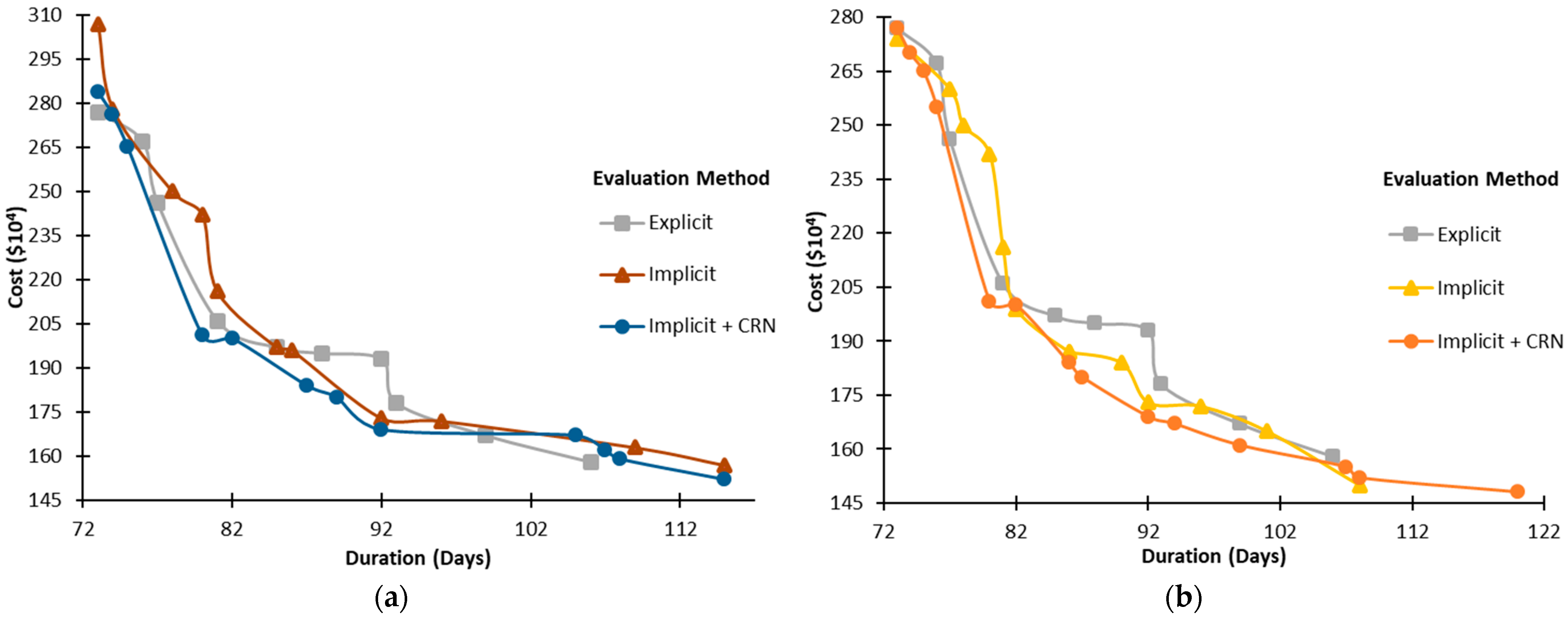
To evaluate the effectiveness of the presented framework, two experiments were carried out. Both experiments were run on an Intel Core i7, Quad-core processor, 3.4 GHz machine with 16 GB RAM. The first experiment compared the performance of EA, IA, and ICRN methods when used to evaluate a fixed number of candidate solutions (i.e., 100,000). The project duration and cost using EA were calculated by averaging 100 simulation replications, whereas 1 simulation replication was used for IA and ICRN. At the end of the optimization, the candidate solutions presented in the best three Pareto fronts of each method were re-evaluated using 1000 replications to obtain accurate statistical information.
Figure 3a shows the final Pareto fronts obtained from the first experiment. The Pareto fronts provided a non-dominated tradeoff between the project duration and cost. When examining the Pareto fronts, it can be noticed that all three methods were able to generate very close Pareto fronts.
Table 1 summarizes the results of both experiments. It took 7.20 h to evaluate 100,000 candidate solutions using EA and 0.65 h for IA and ICRN, which resulted in an average time saving of 91%. Additionally, the ICRN approach achieved a 2.6% and 3.6% improvement in the quality of optimum solutions over EA and IA, respectively, as measured by the hypervolume indicator.
The second experiment compares the performance of three methods when optimization is run for a fixed period of time (i.e., 7.20 h). Since IA and ICRN approaches are faster than EA, they are expected to evaluate far more candidate solutions than EA.
Figure 3b shows the final Pareto fronts obtained in the second experiment. The total number of evaluated candidate solutions by ICRN and IA approaches is 751,415, a 645% increase over the EA approach. ICRN and IA Pareto fronts achieved a 4.9% and 2.9% improvement in the hypervolume indicator, respectively.
4. Conclusions
One of the major drawbacks of the current stochastic simulation optimization frameworks is that they require several simulation replications to evaluate the fitness of the candidate solutions generated by the optimization algorithm. This, in turn, would increase the time and/or computational effort required to solve the optimization problem. To overcome this issue, this paper studied the use of implicit averaging and the joint application of implicit averaging and common random numbers to improve the performance of simulation optimization frameworks.
A box girder bridge project was used to demonstrate the benefits of the presented framework. Based on the study results, the framework reduced the computation time by 91% and improved the quality of optimum solutions by 2.6% when the number of evaluated candidate solutions was fixed. Additionally, the study showed that the presented framework improved the optimization algorithm’s performance by 4.9% and increased the confidence by more than 650%. The initial results of the presented framework showed promise in improving the efficiency and effectiveness of simulation optimization frameworks. For future work, the authors will further investigate the benefits of applying the presented framework to other construction simulation optimization problems.
Author Contributions
Conceptualization, M.M. and F.V.; methodology, M.M. and F.V.; software, M.M. and F.V.; validation, M.M.; formal analysis, M.M. and F.V.; investigation, M.M.; data curation, M.M.; writing—original draft preparation, M.M.; writing—review and editing, F.V. All authors have read and agreed to the published version of the manuscript.
Funding
This research received no external funding.
Institutional Review Board Statement
Not applicable.
Informed Consent Statement
Not applicable.
Data Availability Statement
Some data are available upon request from the corresponding author.
Conflicts of Interest
The authors declare no conflict of interest.
References
- Marzouk, M.; Moselhi, O. Multiobjective optimization of Earthmoving Operations. J. Constr. Eng. Manag. 2004, 103, 105–113. [Google Scholar] [CrossRef]
- Marzouk, M.; Said, H.; El-Said, M. Framework for Multiobjective Optimization of Launching Girder Bridges. J. Constr. Eng. Manag. 2009, 135, 791–800. [Google Scholar] [CrossRef]
- Cheng, M.-Y.; Tran, D.-H. Integrating Chaotic Initialized Opposition Multiple-Objective Differential Evolution and Stochastic Simulation to Optimize Ready-Mixed Concrete Truck Dispatch Schedule. J. Manag. Eng. 2016, 32, 04015034. [Google Scholar] [CrossRef]
- Feng, C.-W.; Liu, L.; Burns, S.A. Stochastic Construction Time-Cost Trade-Off Analysis. J. Comput. Civ. Eng. 2000, 14, 117–126. [Google Scholar] [CrossRef]
- Mawlana, M.; Hammad, A. Integrating Variance Reduction Techniques and Parallel Computing in Construction Simulation Optimization. J. Comput. Civ. Eng. 2019, 33, 04019026. [Google Scholar] [CrossRef]
- Salimi, S.; Mawlana, M.; Hammad, A. Performance analysis of simulation-based optimization of construction projects using High Performance Computing. Autom. Constr. 2018, 87, 158–172. [Google Scholar] [CrossRef]
- Mawlana, M. Improving Stochastic Simulation-Based Optimization for Selecting Construction Method of Precast Box Girder Bridges. Ph.D. Thesis, Concordia University, Montreal, QC, Canada, 2015. [Google Scholar]
- Law, A. Simulation Modeling and Analysis, 4th ed.; McGraw-Hill: Boston, MA, USA, 2007. [Google Scholar]
- Goldberg, D.; Deb, K.; Kaegupta, H.; Harik, G. Rapid, Accurate Optimization of Difficult Problems using Fast Messy Genetic Algorithms. In Proceedings of the Fifth International Conference on Genetic Algorithms, Urbana, IL, USA, 17–21 July 1993. [Google Scholar]
- Zitzler, E.; Thiele, L.; Laumanns, M.; Fonseca, C.M.; Da Fonseca, V.G. Performance assessment of multiobjective optimizers: An analysis and review. IEEE Trans. Evol. Comput. 2003, 7, 117–132. [Google Scholar] [CrossRef]
- Zitzler, E.; Brockhoff, D.; Thiele, L. The hypervolume indicator revisited: On the design of Pareto-compliant indicators via weighted integration. In Evolutionary Multi-Criterion Optimization; Springer: Berlin/Heidelberg, Germany, 2007; pp. 862–876. [Google Scholar] [CrossRef]
- Bradstreet, L. The Hypervolume Indicator for Multi-Objective Optimisation: Calculation and Use. Ph.D. Thesis, The University of Western Australia, Perth, Australia, 2011. [Google Scholar]
- Martínez, J. STROBOSCOPE: State and Resource Based Simulation of Construction Processes. Ph.D. Thesis, University of Michigan, Ann Arbor, MI, USA, 1996. [Google Scholar]
- Wu, Z.Y.; Wang, Q.; Butala, S.; Mi, T. Darwin Optimization Framework User Manual; Bentley Systems Incorporated: Watertown, CT, USA, 2012. [Google Scholar]
| Disclaimer/Publisher’s Note: The statements, opinions and data contained in all publications are solely those of the individual author(s) and contributor(s) and not of MDPI and/or the editor(s). MDPI and/or the editor(s) disclaim responsibility for any injury to people or property resulting from any ideas, methods, instructions or products referred to in the content. |
© 2024 by the authors. Licensee MDPI, Basel, Switzerland. This article is an open access article distributed under the terms and conditions of the Creative Commons Attribution (CC BY) license (https://creativecommons.org/licenses/by/4.0/).


