Analysis of Nanodrug Delivery in Blood Flowing through Blood Vessels Using Machine Learning Models ^†

Abstract

This study provides a framework to strategize localized efficient drug delivery in second-order blood flowing through porous blood vessels using machine learning algorithms. With the assumption of long blood vessels, the flow-governing equation, the Navier–Stokes equation, is reduced to a simpler model which is consistent with the lubrication theory. We solved this equation analytically with slip conditions and obtained the analytical expression of the velocity profile for the Newtonian model. We modelled the concentration of nanodrugs with an advection diffusion equation to analyze the effect of concentration on the localized disease. The particle concentration at the blood vessel wall was evaluated using the finite-difference method. To analyze the particle concentration, we implemented machine learning algorithms including Gradient Boost, XG Boost, Regression Tree, MLP Regressor, and CatBoost Regressor. Our conclusion predicts the optimum machine learning algorithm for transferring the delivery of the nanoparticle drug.

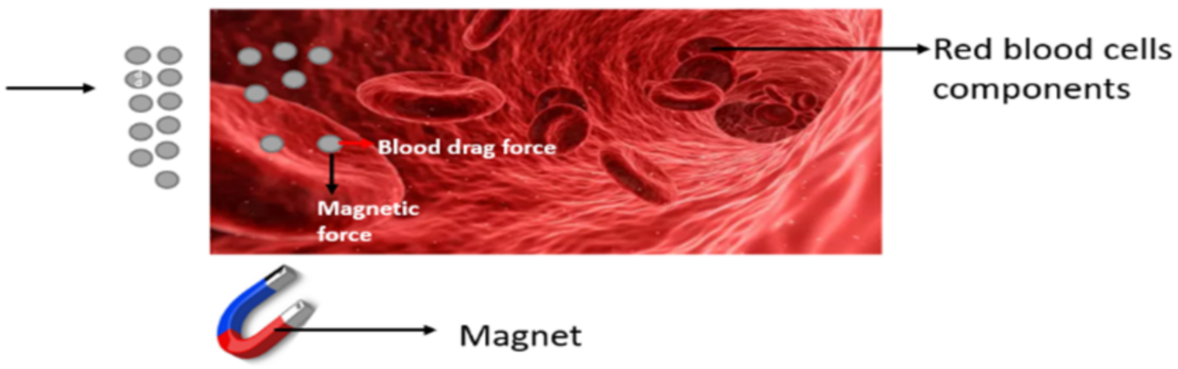
1. Introduction

Treating diseases localized to a particular tissue is quite challenging through medication. In order to cure various human diseases in an efficient way, drug delivery is gaining a lot of attention in the field of medicine. Conventionally, these drugs are delivered at a slow, controlled rate and administered through intravenous injection. Drug delivery comprising nanoparticles improves the impact and efficiency of its application. Nanoparticles are capable of delivering drugs to the localized infected cells and minimize the leakage of the drug to the non-infected cells (Figure 1). Magnetic nanoparticles are nanoparticles under the impact of a magnetic field. These magnetic nanoparticles can be manipulated by an external magnet.

In the field of biomedicine, a magnetic drug carrier is injected through the blood vessel to the infected cell location under the influence of an external magnetic field. Pankhurst et al. [1] studied the application of magnetic nanoparticles. Using magnetic nanoparticles, Andrew and Richardson [2] mathematically modelled a drug-delivery method that is capable of tracking nanoparticles in the blood vessels. They investigated and showed that it is not possible to specify the target of the internal regions with the help of an external magnetic field. Under the impact of an external magnetic field, Iris et al. [3] studied a mathematical model in order to track each super-magnetic nanoparticle in the blood flow. Their study was mainly on treating localized cancer. Nadeem and Iijaz [4] analyzed the blood flow of a stenosed curved artery in the presence of nanoparticles. They considered the channel to be curved and the walls to be permeable. The governing equations under the impact of mild stenosis were solved by taking the appropriate boundary conditions. Under the impact of magnetic field, Nacev et al. [5] studied the behavior of ferromagnetic nanoparticles in the blood vessels. These particles are governed by blood diffusion, convection, and extravasation. Controlled drug delivery with magnetic nanoparticles in the blood was presented by Abu-Hamdel Nidal et al. [6]. Blood was assumed to be a non-Newtonian fluid. They used the Navier–Stokes equation and Maxwell equation to solve the system. Bhatti et al. [7] investigated the flow of nanofluid comprising copper and gold nanoparticles. Their study aimed to transport the magnetic drug through the stenosed artery. Sutterby fluid acted as a base fluid that was non-Newtonian in nature. Tiam et al. [8] analyzed the linear stability of blood flow consisting of magnetic nanoparticles and investigated the controlled drug delivery taking place in a porous artery in the presence of a magnetic field. Their study placed importance on controlling the mobility of the nanoparticles. Ponalagusamy et al. [9] studied a mathematical model for a flow with periodic variations. They considered blood to be a Bingham fluid and their method involved movement of magnetic particles through an infected artery. Hiwa et al. [10] studied a method to improve drug delivery to the targeted area in a carotid bifurcation. To solve the numerical simulation, they employed the Eulerian–Lagrangian method and finite-element method, Dubey et al. [11] investigated a 2D study of an infected permeable artery consisting of mild stenosis and an aneurysm (a condition which causes the artery wall to balloon up at a weak spot). The blood flow was affected by the metallic nanoparticles. Vasu et al. [12] developed a mathematical model for an infected tapered artery with nanoparticles. The artery had a mild stenosis present and various metallic nanoparticles were immersed into the blood. The Eringen micropolar model was used to characterize the region of the artery. The effect of copper and silver nanoparticles in a catheterized tapered inclined artery with stenosis and aneurysm was presented by Jayati et al. [13]. The transformed equations were solved by the FTCS method. Jayati et al. [14] numerically simulated the transport of nanoparticles in hydromagnetic blood flow in order to treat arterial diseases. The diseased artery included a composite stenosis and an irregular stenosis. The governing equations were solved by FDM in which an explicit FTCS technique was employed. Aparna et al. [15] formulated and evaluated magnesium sulphate nanoparticles which improved the penetrability of CNS. Misra and Shit [16] studied the role of slip velocity in the flow of blood in a stenosed artery. The Herschel–Bulkley equation was used to describe the flow. Ragima et al. [17] analyzed how blood is compatible with chitosan. Asha and Neetu [18] studied the stenosis geometry and the effect of blood flowing through an artery under various conditions. Claudia et al. [19] investigated the effect of nanodrug delivery with magnetic effect in non-Newtonian blood flow. They analyzed the effect of shear thinning with Newtonian power-law, Ellis, and Carreau fluids. Numerical techniques were implemented to solve the system. Selladurai et al. [20] studied the impact of shear stress over a symmetric stenosed artery wall with the effect of magnetic field. They implemented machine learning models to measure the best accuracy to predict the shear stress.

In this paper, we consider blood to be Newtonian to strategize localized efficient drug delivery in second-order blood flowing through porous blood vessels. The concentration of the nanoparticles was evaluated using the finite-difference method and analysed using five machine learning algorithms: Gradient Boost, XG Boost 2.0.1, Regression Tree, MLP Regressor, and CatBoost Regressor. The accuracy of the models was compared using statistical accuracy measures.

2. Formulation of the Problem

Consider the blood vessel to be a long and thin rectangular channel which is consistent with the size of the blood vessels in the human body (Figure 1). The vector form of the governing equation which describes the flow is given by (1) and (2) as follows:

$$\mathsf{\rho }\left[\frac{\partial {\mathrm{U}}_{\mathrm{f}}}{\partial \mathrm{t}}+{\mathrm{U}}_{\mathrm{f}}.\nabla {\mathrm{U}}_{\mathrm{f}}\right]=-\nabla \mathrm{p}+\nabla .\mathsf{\tau }+{\mathrm{F}}_{\mathrm{m}\mathrm{a}\mathrm{g}},$$

(1)

$$\nabla .{\mathrm{U}}_{\mathrm{f}}=0$$

(2)

where ${\mathrm{U}}_{\mathrm{f}}$ is the fluid velocity, $\mathsf{\rho }$ is density of the fluid, $\mathrm{p}$ is pressure, $\mathsf{\tau }$ is the shear stress, and ${\mathrm{F}}_{\mathrm{m}\mathrm{a}\mathrm{g}}$ is force due to the external magnet.

Let us consider the nanofluid to be dilute in nature. Blood is paramagnetic in nature and the capacity of the nanoparticles to alter the flow rheology becomes negligible; hence we can assume ${\mathrm{F}}_{\mathrm{m}\mathrm{a}\mathrm{g}}0$.

Shear stress for the power law model can be written as follows:

$${\mathsf{\tau }}_{\mathrm{y}\mathrm{x}}=\mathsf{\mu }{\left|\frac{\partial {\mathrm{U}}_{\mathrm{f}}}{\partial \mathrm{y}}\right|}^{{\mathrm{n}}_{\mathrm{p}}}$$

(3)

where for ${\mathrm{n}}_{\mathrm{p}}$ = 1 it becomes Newtonian. So, we investigated the Newtonian case.

• Expressing (1) and (2) component-wise we obtain:

$$\frac{\partial {\mathrm{u}}_{\mathrm{f}}}{\partial \mathrm{x}}+\frac{\partial {\mathrm{v}}_{\mathrm{f}}}{\partial \mathrm{y}}=0,$$

(4)

$$\frac{\partial {\mathrm{u}}_{\mathrm{f}}}{\partial \mathrm{t}}+{\mathrm{u}}_{\mathrm{f}}\frac{\partial {\mathrm{u}}_{\mathrm{f}}}{\partial \mathrm{x}}+{\mathrm{v}}_{\mathrm{f}}\frac{\partial {\mathrm{u}}_{\mathrm{f}}}{\partial \mathrm{y}}=-\frac{1}{\mathsf{\rho }}\frac{\partial \mathrm{p}}{\partial \mathrm{x}}+\frac{1}{\mathsf{\rho }}\left[\frac{\partial {\mathsf{\tau }}_{\mathrm{x}\mathrm{x}}}{\partial \mathrm{x}}+\frac{\partial {\mathsf{\tau }}_{\mathrm{y}\mathrm{x}}}{\partial \mathrm{y}}\right],$$

(5)

$$\frac{\partial {\mathrm{v}}_{\mathrm{f}}}{\partial \mathrm{t}}+{\mathrm{u}}_{\mathrm{f}}\frac{\partial {\mathrm{v}}_{\mathrm{f}}}{\partial \mathrm{x}}+{\mathrm{v}}_{\mathrm{f}}\frac{\partial {\mathrm{v}}_{\mathrm{f}}}{\partial \mathrm{y}}=-\frac{1}{\mathsf{\rho }}\frac{\partial \mathrm{p}}{\partial \mathrm{y}}+\frac{1}{\mathsf{\rho }}\left[\frac{\partial {\mathsf{\tau }}_{\mathrm{x}\mathrm{y}}}{\partial \mathrm{x}}+\frac{\partial {\mathsf{\tau }}_{\mathrm{y}\mathrm{y}}}{\partial \mathrm{y}}\right]$$

(6)

where ${\mathrm{u}}_{\mathrm{f}},{\mathrm{v}}_{\mathrm{f}}$ are the components of fluid velocity along the x and y directions.

The boundary conditions for the problem can be written as follows:

$$\frac{\partial {\mathrm{u}}_{\mathrm{f}}}{\partial \mathrm{y}}=0 \mathrm{a}\mathrm{t} \mathrm{y}=0, {\mathrm{u}}_{\mathrm{f}}={\mathrm{U}}_{\mathrm{B}} \mathrm{a}\mathrm{t} \mathrm{y}=\mathrm{R}$$

(7)

For non-dimensionalising the resulting equations, the following equations are used:

$$\mathrm{x}=\mathrm{L}\widehat{\mathrm{x}},\mathrm{y}=2\mathrm{R}\mathrm{L}\widehat{\mathrm{y}},{\mathrm{u}}_{\mathrm{f}}=\mathrm{U}{\widehat{\mathrm{u}}}_{\mathrm{f}},{\mathrm{v}}_{\mathrm{f}}=\mathrm{V}\mathrm{L}{\widehat{\mathrm{v}}}_{\mathrm{f}},\mathrm{p}=\mathrm{P}\widehat{\mathrm{p}},\mathsf{\tau }=\mathsf{{\rm T}}\widehat{\mathsf{\tau }}$$

(8)

In order to balance the terms in (4), we take ${\mathrm{v}}_{\mathrm{f}}=\mathsf{ϵ}{\mathrm{u}}_{\mathrm{f}}$, where $\mathsf{ϵ}=\frac{2\mathrm{r}}{\mathrm{l}}\ll 1$ (because the vessels are considered to be thin and long).

We obtain the following dimensionless equation:

$$\frac{\partial {\widehat{\mathrm{u}}}_{\mathrm{f}}}{\partial \widehat{\mathrm{x}}}+\frac{\partial {\widehat{\mathrm{v}}}_{\mathrm{f}}}{\partial \widehat{\mathrm{y}}}=0$$

(9)

Taking $\mathrm{P}=\frac{\mathrm{l}\mathrm{T}}{2\mathrm{r}}$ and considering a steady state, we obtain:

$$\frac{\mathsf{\rho }\mathsf{ϵ}{\mathrm{U}}^2}{\mathrm{T}}\left[{\widehat{\mathrm{u}}}_{\mathrm{f}}\frac{\partial {\widehat{\mathrm{u}}}_{\mathrm{f}}}{\partial \widehat{\mathrm{x}}}+{\widehat{\mathrm{v}}}_{\mathrm{f}}\frac{\partial {\widehat{\mathrm{v}}}_{\mathrm{f}}}{\partial \widehat{\mathrm{y}}}\right] =-\frac{\partial \widehat{\mathrm{p}}}{\partial \widehat{\mathrm{x}}}+\mathsf{ϵ}\frac{\partial \widehat{\mathsf{\tau }}{}_{\widehat{\mathrm{x}}\widehat{\mathrm{x}}}}{\partial \widehat{\mathrm{x}}}+\frac{\partial \widehat{\mathsf{\tau }}{}_{\widehat{\mathrm{y}}\widehat{\mathrm{x}}}}{\partial \widehat{\mathrm{y}}},$$

(10)

$$\frac{\mathsf{\rho }\mathsf{ϵ}{\mathrm{U}}^2}{\mathrm{T}}\left[{\widehat{\mathrm{u}}}_{\mathrm{f}}\frac{\partial {\widehat{\mathrm{u}}}_{\mathrm{f}}}{\partial \widehat{\mathrm{x}}}+{\widehat{\mathrm{v}}}_{\mathrm{f}}\frac{\partial {\widehat{\mathrm{v}}}_{\mathrm{f}}}{\partial \widehat{\mathrm{y}}}\right]=-\frac{\partial \widehat{\mathrm{p}}}{\partial \widehat{\mathrm{y}}}+{\mathsf{ϵ}}^2\frac{\partial \widehat{\mathsf{\tau }}{}_{\widehat{\mathrm{x}}\widehat{\mathrm{y}}}}{\partial \widehat{\mathrm{x}}}+\mathsf{ϵ}\frac{\partial \widehat{\mathsf{\tau }}{}_{\widehat{\mathrm{y}}\widehat{\mathrm{y}}}}{\partial \widehat{\mathrm{y}}}$$

(11)

Let us assume that $\frac{\mathsf{\rho }\mathsf{ϵ}{\mathrm{U}}^2}{\mathrm{T}}\ll 1$. Hence, we obtain the following equations in dimensional form:

$$\frac{\partial {\mathrm{u}}_{\mathrm{f}}}{\partial \mathrm{x}}+\frac{\partial {\mathrm{v}}_{\mathrm{f}}}{\partial \mathrm{x}}=0,$$

(12)

$$\frac{\partial \mathrm{p}}{\partial \mathrm{x}}=\frac{\partial {\mathsf{\tau }}_{\mathrm{y}\mathrm{x}}}{\partial \mathrm{y}},$$

(13)

$$\frac{\partial \mathrm{p}}{\partial \mathrm{y}}=0$$

(14)

3. Solution for the Newtonian Model

On substituting (3) in (13) and integrating (13) twice with respect to y, we obtain the velocity expression as follows:

$${\mathrm{U}}_{\mathrm{f}}\left(\mathrm{y}\right)=\frac{3}{2{\mathrm{R}}^2}\left(-\frac{\mathrm{Q}}{2\mathrm{R}}+{\mathrm{U}}_{\mathrm{B}}\right)\left({\mathrm{y}}^2-{\mathrm{R}}^2\right)+{\mathrm{U}}_{\mathrm{B}}$$

(15)

where $Q$ is the flow rate and is determined by the expression:

$$\mathrm{Q}={\int }_{-\mathrm{R}}^{\mathrm{R}}{\mathrm{U}}_{\mathrm{f}}\mathrm{d}\mathrm{y}$$

(15a)

The corresponding shear stress is given by:

$${\mathsf{\tau }}_{\mathrm{y}\mathrm{x}}=\mathsf{\mu }\frac{\mathrm{d}{\mathrm{U}}_{\mathrm{f}}}{\mathrm{d}\mathrm{y}}=\mathsf{\mu }\frac{3\mathrm{y}}{{\mathrm{R}}^2}\left({\mathrm{U}}_{\mathrm{B}}-\frac{\mathrm{Q}}{2\mathrm{R}}\right)$$

(16)

4. Modelling of the Concentration of Nano Drug Particle

The nanoparticle concentration $\mathbf{c}(\mathrm{x},\mathrm{y},\mathrm{t})$ is given by the advection–diffusion equation:

$$\frac{\partial \mathbf{c}}{\partial \mathrm{t}}+\nabla .[{(\mathrm{U}}_{\mathrm{f}}+{\mathrm{V}}_{\mathrm{p}})\mathbf{c}]=\nabla . {\mathrm{J}}_{\mathrm{d}\mathrm{i}\mathrm{f}\mathrm{f}}$$

(17)

where ${\mathrm{U}}_{\mathrm{f}}$ is velocity of the fluid, ${\mathrm{V}}_{\mathrm{p}}$ is the particle velocity, and ${\mathrm{J}}_{\mathrm{d}\mathrm{i}\mathrm{f}\mathrm{f}}$ = $-\mathrm{D}\nabla \mathbf{c}$ is the flux of diffusion. On substituting the expression of ${\mathrm{J}}_{\mathrm{d}\mathrm{i}\mathrm{f}\mathrm{f}}$, Equation (17) takes a form as follows:

$$\frac{\partial \mathbf{c}}{\partial \mathrm{t}}+{\mathrm{U}}_{\mathrm{f}}\frac{\partial \mathbf{c}}{\partial \mathrm{x}}+\frac{\partial \left({\mathrm{V}}_{\mathrm{p}}\mathbf{c}\right)}{\partial \mathrm{y}}=\mathrm{D}\frac{{\partial }^2\mathbf{c}}{\partial {\mathrm{x}}^2}+\frac{\partial }{\partial \mathrm{y}}\left(\mathrm{D}\frac{\partial \mathbf{c}}{\partial \mathrm{y}}\right)$$

(18)

We assume the nanoparticles enter the vessel at an injection of 3 s near the vicinity of $x=0;$ hence, we have

$${\mathrm{U}}_{\mathrm{f}}{\mathbf{c}}_{\mathbf{i}\mathbf{n}}\left(\mathrm{y},\mathrm{t}\right)=\left({\mathrm{U}}_{\mathrm{f}}\mathbf{c}-\mathrm{D}\frac{\partial \mathbf{c}}{\partial \mathrm{x}}\right) \mathrm{on} \mathrm{x}=0$$

(19)

The distribution of the concentration of the nanoparticles entering the blood vessel is ${\mathbf{c}}_{\mathbf{i}\mathbf{n}}\left(\mathrm{y},\mathrm{t}\right)$ and can be written as follows:

$${\mathbf{c}}_{\mathbf{i}\mathbf{n}}\left(\mathrm{y},\mathrm{t}\right)=\frac{\mathrm{g}\left(\mathrm{t}\right)}{4}\mathrm{e}\mathrm{r}\mathrm{f}\mathrm{c}\left[\frac{\mathrm{S}}{2\mathrm{R}}\left(\mathrm{y}-\frac{\mathrm{R}}{3}\right)\right]\left\{1+\mathrm{e}\mathrm{r}\mathrm{f}\mathrm{c}\left[\frac{\mathrm{S}}{2\mathrm{R}}\left(\mathrm{y}+\frac{\mathrm{R}}{3}\right)\right]\right\}{\mathbf{c}}_0$$

(20)

where g(t) = $\frac{\mathrm{t}}{3}$, t ranges from 0 to 3 s, and S is a parameter controlling the steepness of the error function (erfc).

$${\mathbf{c}}_{\mathbf{i}\mathbf{n}}\left(\mathrm{y},\mathrm{t}\right)=0 \mathrm{when}\mathrm{t}>3 \mathrm{s}$$

(21)

At the channel outlet:

$${\mathrm{U}}_{\mathrm{f}} \left(\mathbf{c}-\mathrm{D}\frac{\partial \mathbf{c}}{\partial \mathrm{x}}\right)=0 \mathrm{on} \mathrm{x}=\mathrm{L}$$

(22)

At the vessel wall:

$${(\mathrm{u}}_{\mathrm{t}\mathrm{o}\mathrm{t}}\mathbf{c}-\mathrm{D} \nabla \mathbf{c}).\mathrm{n}=\mathsf{\kappa }\mathbf{c} \mathrm{o}\mathrm{n} \mathrm{y}=\pm \mathrm{R}$$

(23)

where $u_{tot}=\left({\mathrm{U}}_{\mathrm{f}}\left(\mathrm{y}\right),{\mathrm{V}}_{\mathrm{p}}\left(\mathrm{y}\right)\right),$ $\kappa$ is permeability of the blood vessel wall.

Let us introduce dimensionless parameters as follows:

$$\mathrm{t}=\mathsf{\delta }\mathrm{t}\widehat{\mathrm{t}},\mathbf{c}={\mathbf{c}}_{\mathbf{0}}\widehat{\mathbf{c}},{\mathrm{U}}_{\mathrm{f}}=\mathrm{U}{\widehat{\mathrm{U}}}_{\mathrm{f}},{\mathrm{V}}_{\mathrm{p}}=\mathrm{W}\widehat{{\mathrm{V}}_{\mathrm{p}}},\mathrm{D}=\overline{\mathrm{D}}\widehat{\mathrm{D}}$$

(24)

Substituting Equation (8) into Equation (18) we obtain the following equation:

$$\frac{{\mathbf{c}}_{\mathbf{0}}}{\mathsf{\delta }\mathrm{t}}\frac{\partial \widehat{\mathrm{c}}}{\partial \widehat{\mathrm{t}}}+\frac{\mathrm{U}{\mathbf{c}}_{\mathbf{0}}}{\mathrm{L}}{\widehat{\mathrm{U}}}_{\mathrm{f}}\frac{\partial \widehat{\mathbf{c}}}{\partial \widehat{\mathrm{x}}}+\frac{\mathrm{W}{\mathbf{c}}_{\mathbf{0}}}{2\mathrm{R}}\frac{\partial \left({\widehat{\mathrm{V}}}_{\mathrm{p}}\widehat{\mathrm{c}}\right)}{\partial \widehat{\mathrm{y}}}=\frac{\overline{\mathrm{D}}}{{\mathrm{L}}^2}{\mathbf{c}}_{\mathbf{0}}\left(\widehat{\mathrm{D}}\frac{{\partial }^2\widehat{\mathbf{c}}}{\partial {\mathrm{x}}^2}\right)+\frac{\overline{\mathrm{D}}}{4{\mathrm{R}}^2}\frac{\partial }{\partial \widehat{\mathrm{y}}}\left(\widehat{\mathrm{D}}\frac{\partial \widehat{\mathbf{c}}}{\partial \widehat{\mathrm{y}}}\right)$$

(25)

where U = $\mathrm{m}\mathrm{a}\mathrm{x}\left({\mathrm{U}}_{\mathrm{f}}\right)$, $\overline{\mathrm{D}}=\mathrm{m}\mathrm{a}\mathrm{x}\left(\mathrm{D}\right)$.

On simplifying and taking $\delta t=\frac{L}{U}$ in order to balance out the derivative term of time with the advection term, our equation takes the form as follows:

$$\frac{\partial \widehat{\mathbf{c}}}{\partial \widehat{\mathrm{t}}}+{\widehat{\mathrm{U}}}_{\mathrm{f}}\frac{\partial \widehat{\mathbf{c}}}{\partial \widehat{\mathrm{x}}}+\frac{\mathsf{\delta }}{\mathsf{ϵ}}\frac{\partial \left({\widehat{\mathrm{V}}}_{\mathrm{p}}\widehat{\mathbf{c}}\right)}{\partial \widehat{\mathrm{y}}}=\frac{1}{\mathsf{ϵ}\mathrm{P}\mathrm{e}}\left[{\mathsf{ϵ}}^2\left(\widehat{\mathrm{D}}\frac{{\partial }^2\widehat{\mathbf{c}}}{\partial {\mathrm{x}}^2}\right)+\frac{\partial }{\partial \widehat{\mathrm{y}}}\left(\widehat{\mathrm{D}}\frac{\partial \widehat{\mathbf{c}}}{\partial \widehat{\mathrm{y}}}\right)\right]$$

(26)

The boundary conditions at the vessel wall can be written as follows:

$${\widehat{\mathrm{V}}}_{\mathrm{p}}\widehat{\mathbf{c}}-\frac{1}{\mathrm{P}\mathrm{e}\mathsf{\delta }}\widehat{\mathrm{D}}\frac{\partial \widehat{\mathbf{c}}}{\partial \widehat{\mathrm{y}}}=\pm \mathrm{h}\widehat{\mathbf{c}}\mathrm{on} \widehat{\mathrm{y}}=\pm 1/2$$

(27)

where $\mathrm{h}=\frac{\mathsf{\kappa }}{\mathrm{W}},\mathrm{W} \mathrm{i}\mathrm{s} \mathrm{m}\mathrm{a}\mathrm{x}{(\mathrm{V}}_{\mathrm{f}})$.

At the inlet:

$${\widehat{\mathrm{U}}}_{\mathrm{f}}\widehat{\mathbf{c}}-\frac{\mathsf{ϵ}}{\mathrm{P}\mathrm{e}}\widehat{\mathrm{D}}\frac{\partial \widehat{\mathbf{c}}}{\partial \widehat{\mathrm{x}}}=0 \mathrm{on} \widehat{\mathrm{x}}=1$$

(28)

At the outlet:

$${\widehat{\mathrm{U}}}_{\mathrm{f}}\widehat{\mathbf{c}}-\frac{\mathsf{ϵ}}{\mathrm{P}\mathrm{e}}\widehat{\mathrm{D}}\frac{\partial \widehat{\mathbf{c}}}{\partial \widehat{\mathrm{x}}}=0 \mathrm{on} \widehat{\mathrm{x}}=1$$

(29)

Finite Difference Method

• Dropping the hats in (26)–(29) and defining:

$${\mathbf{c}}_{\mathrm{i},\mathrm{j}}^{\mathrm{n}}≔\mathbf{c}\left({\mathrm{x}}_{\mathrm{i}},{\mathrm{y}}_{\mathrm{j},}{\mathrm{t}}^{\mathrm{n}}\right),{\mathrm{U}}_{{\mathrm{f}}_{\mathrm{j}}}≔{\mathrm{U}}_{\mathrm{f}}\left({\mathrm{y}}_{\mathrm{j}}\right),{\mathrm{V}}_{{\mathrm{f}}_{\mathrm{j}}}≔{\mathrm{V}}_{\mathrm{p}}\left({\mathrm{y}}_{\mathrm{j}}\right),{\mathrm{D}}_{{\mathrm{T}}_{\mathrm{j}}}≔\mathrm{D}\left({\mathrm{y}}_{\mathrm{j}}\right)$$

(30)

$$\begin{gathered} \frac{{\mathbf{c}}_{\mathrm{i},\mathrm{j}}^{\mathrm{n}+1}-{\mathbf{c}}_{\mathrm{i},\mathrm{j}}^{\mathrm{n}}}{\Delta \mathrm{t}}+{\mathrm{U}}_{{\mathrm{F}}_{\mathrm{j}}}\left(\frac{{\mathbf{c}}_{\mathrm{i},\mathrm{j}}^{\mathrm{n}}-{\mathbf{c}}_{\mathrm{i}-1,\mathrm{j}}^{\mathrm{n}}}{\Delta \mathrm{x}}\right)+\frac{\mathsf{\delta }}{\mathsf{ϵ}}\left(\frac{{\mathrm{V}}_{{\mathrm{p}}_{\mathrm{j}+1}}{\mathbf{c}}_{\mathrm{i},\mathrm{j}+1}^{\mathrm{n}}-{\mathrm{V}}_{{\mathrm{p}}_{\mathrm{j}}}{\mathbf{c}}_{\mathrm{i},\mathrm{j}}^{\mathrm{n}}}{\Delta \mathrm{y}}\right) = \frac{{\mathrm{D}}_{{\mathrm{T}}_{\mathrm{j}+1/2}}}{\mathsf{ϵ}\mathrm{P}\mathrm{e}}\left(\frac{{\mathbf{c}}_{\mathrm{i},\mathrm{j}+1}^{\mathrm{n}}-{\mathbf{c}}_{\mathrm{i},\mathrm{j}}^{\mathrm{n}}}{{\Delta \mathrm{y}}^2}\right)+\frac{\mathsf{ϵ}}{\mathrm{P}\mathrm{e}} - \\ \hspace{1em}\hspace{1em}\hspace{1em}\hspace{1em}\hspace{1em}\hspace{1em}\hspace{1em}\hspace{1em}\hspace{1em}\hspace{1em} {\mathrm{D}}_{{\mathrm{T}}_{\mathrm{j}}}\left(\frac{{\mathbf{c}}_{\mathrm{i}+1,\mathrm{j}}^{\mathrm{n}}-2{\mathbf{c}}_{\mathrm{i},\mathrm{j}}^{\mathrm{n}}+{\mathbf{c}}_{\mathrm{i}-1,\mathrm{j}}^{\mathrm{n}}}{{\Delta \mathrm{x}}^2}\right)+\frac{{\mathrm{D}}_{{\mathrm{T}}_{\mathrm{j}-1/2}}}{\mathsf{ϵ}\mathrm{P}\mathrm{e}}\left(\frac{{\mathbf{c}}_{\mathrm{i},\mathrm{j}}^{\mathrm{n}}-{\mathbf{c}}_{\mathrm{i},\mathrm{j}-1}^{\mathrm{n}}}{{\Delta \mathrm{y}}^2}\right) \end{gathered}$$

(31)

At the inlet:

$${\mathrm{U}}_{{\mathrm{F}}_{\mathrm{j}}}{\mathrm{c}}_{\mathrm{i}\mathrm{n},\mathrm{j}}^{\mathrm{n}+1}={\mathrm{U}}_{{\mathrm{F}}_{\mathrm{j}}}{\mathbf{c}}_{1,\mathrm{j}}^{\mathrm{n}+1}-\frac{\mathsf{ϵ}}{\mathrm{P}\mathrm{e}}-{\mathrm{D}}_{{\mathrm{T}}_{\mathrm{j}}}\left(\frac{-{\mathbf{c}}_{3,\mathrm{j}}^{\mathrm{n}+1}+4{\mathbf{c}}_{2,\mathrm{j}}^{\mathrm{n}+1}-3{\mathbf{c}}_{1,\mathrm{j}}^{\mathrm{n}+1}}{2\Delta \mathrm{x}}\right)$$

(32)

At the outlet:

$${\mathrm{U}}_{{\mathrm{F}}_{\mathrm{j}}}{\mathbf{c}}_{{\mathrm{n}}_{\mathrm{x}},\mathrm{j}}^{\mathrm{n}+1}-\frac{\mathsf{ϵ}}{\mathrm{P}\mathrm{e}}-{\mathrm{D}}_{{\mathrm{T}}_{\mathrm{j}}}\left(\frac{-{\mathbf{c}}_{{\mathrm{n}}_{\mathrm{x}-2},\mathrm{j}}^{\mathrm{n}+1}+4{\mathbf{c}}_{{\mathrm{n}}_{\mathrm{x}-1},\mathrm{j}}^{\mathrm{n}+1}-3{\mathbf{c}}_{{\mathrm{n}}_{\mathrm{x}},\mathrm{j}}^{\mathrm{n}+1}}{2\Delta \mathrm{x}}\right)=0$$

(33)

At the vessel wall:

$${\mathrm{V}}_{{\mathrm{p}}_{{\mathrm{n}}_{\mathrm{y}}}}{\mathbf{c}}_{\mathrm{i},{\mathrm{n}}_{\mathrm{y}}}^{\mathrm{n}+1}-\frac{1}{\mathrm{P}\mathrm{e}\mathsf{\delta }}{\mathrm{D}}_{{\mathrm{T}}_{{\mathrm{n}}_{\mathrm{y}}}}\left(\frac{3{\mathbf{c}}_{\mathrm{i},{\mathrm{n}}_{\mathrm{y}}}^{\mathrm{n}+1}-4{\mathbf{c}}_{\mathrm{i},{\mathrm{n}}_{\mathrm{y}}-1}^{\mathrm{n}+1}+{\mathbf{c}}_{\mathrm{i},{\mathrm{n}}_{\mathrm{y}}-2}^{\mathrm{n}+1}}{2\Delta \mathrm{y}}\right)=\mathrm{h} {\mathbf{c}}_{\mathrm{i},{\mathrm{n}}_{\mathrm{y}}}^{\mathrm{n}+1},$$

(34)

$${\mathrm{V}}_{{\mathrm{p}}_{{\mathrm{n}}_{\mathrm{y}}}}{\mathbf{c}}_{\mathrm{i},{\mathrm{n}}_{\mathrm{y}}}^{\mathrm{n}+1}-\frac{1}{\mathrm{P}\mathrm{e}\mathsf{\delta }}{\mathrm{D}}_{{\mathrm{T}}_{{\mathrm{n}}_{\mathrm{y}}}}\left(\frac{3{\mathbf{c}}_{\mathrm{i},{\mathrm{n}}_{\mathrm{y}}}^{\mathrm{n}+1}-4{\mathbf{c}}_{\mathrm{i},{\mathrm{n}}_{\mathrm{y}}-1}^{\mathrm{n}+1}+{\mathbf{c}}_{\mathrm{i},{\mathrm{n}}_{\mathrm{y}}-2}^{\mathrm{n}+1}}{2\Delta \mathrm{y}}\right)=\mathrm{h} {\mathbf{c}}_{\mathrm{i},{\mathrm{n}}_{\mathrm{y}}}^{\mathrm{n}+1}$$

(35)

where $\mathsf{ϵ}\ll 1$.

The solution expression for the time step 1 and 2 at the node (1,1) can be written as follows:

$${\mathbf{c}}_{\mathrm{1,1}}^1=0,$$

(36)

$${\mathbf{c}}_{\mathrm{1,1}}^2=\Delta \mathrm{t}\left(\frac{{\mathrm{U}}_{{\mathrm{F}}_1}}{\mathrm{r}\Delta \mathrm{x}}-\frac{\mathsf{\delta }}{\mathsf{ϵ}}\frac{{\mathrm{V}}_{{\mathrm{p}}_2}}{\Delta \mathrm{y}}+\frac{1}{\mathsf{ϵ}\mathrm{P}\mathrm{e}}\frac{{\mathrm{D}}_{{\mathrm{T}}_{3/2}}}{{\Delta \mathrm{y}}^2}–\left(1+\frac{1}{\mathrm{r}}\right)\frac{1}{\mathsf{ϵ}\mathrm{P}\mathrm{e}}\frac{{\mathrm{D}}_{{\mathrm{T}}_{1/2}}}{{\Delta \mathrm{y}}^2}\right)$$

(37)

We can evaluate all nodes similarly.

5. Description of the Data

The formulation of the mathematical model was solved using an analytical method. The data were generated using the explicit relations obtained as a result of solutions to the formulations. The data comprised 100 values with information on pressure gradient, flow rate, y coordinate, fluid velocity ${\mathbf{U}}_{\mathbf{f}}$, shear rate, and concentration.

6. Machine Learning Modelling

6.1. Multilayer Perceptron (MLP)

Models comprising of an artificial neural network (ANN) are inspired by the brain. One of the ANN models is the perceptron. It is comprised of three layers. The input layer consists of features like y, fluid velocity ${\mathrm{U}}_{\mathrm{f}}$, shear rate, and shear stress. The input layer receives the signal and passes through a rectified linear activation function (ReLu). Three hidden layers with 20 nodes are added, which helps to improve the performance and accuracy of the model. The output layer comprises the concentration of the nanoparticles. The learning rate is taken to be a constant.

6.2. Decision Tree

A decision tree is a flow-chart-like model in which each branch node represents a choice between a number of alternatives, and each leaf node represents a decision. Fluid velocity is taken as the root node and many trees can be fitted depending on this node. The root node is split continuously until homogeneous or until a decision is reached without confusion. The depth of the decision tree was chosen to be seven, and the maximum number of leaf nodes was chosen to be 25. The accuracy of the decision tree is predicted by root-mean-square error. The highest root-mean-square error (RMSE) is split continuously till it reaches zero squared error and the algorithm is stopped. The decision tree becomes stable after seven branches.

6.3. Gradient Boosting Regressor

The Gradient Boosting Regressor produced a predictive model to predict the concentration of the nanodrug from an ensemble of weak predictive models. The maximum number of leaf nodes was chosen to be 15, with a minimum of two sampled leaves. Squared error is the loss function. The learning rate was taken to be 0.03, to improve the accuracy of the model.

6.4. XG (Extreme Gradient) Boost Regressor

The XG Boost regressor is a more regularized form of Gradient Boosting Regressor. It is an implementation of gradient boosting. As the model is fit, the loss is minimized. The number of boosting stages is taken to be 15 with 20 nodes in each tree. Learning rate is chosen to be 0.2 which improves the performance of the model.

6.5. CatBoost Regressor

CatBoost grows trees by imposing a rule that all nodes are at the same level. The model reduces the errors by learning the mistakes of the former trees formed. RMSE is utilized as the performance function. We implemented this model to predict the concentration of the nanodrug, with the input variables taken as y, fluid velocity $U_f$, shear rate, and shear stress. The learning rate was set to 0.026897.

7. Statistical Accuracy Metrics

To evaluate the performance metric, we implemented root-mean-square error, coefficient of determination $R^2,$ AARD, and standard deviation (STD). $R^2$ gives us information about the goodness of fit for our dataset. It represents how scattered our observed values are around the regression line. A high value of $R^2$ indicates a better fit. $R^2$ ranges between 0 and 1. When $R^2$ takes the value 1, the model is a perfect fit. Root-mean-square error is the measure of the error a model gives while predicting the data. A lower RMSE value indicates that the model is well optimized and gives a better fit. AARD takes the average deviation using absolute values from the mean of the dataset. Standard deviation (STD) is a measure that gives us information about how spread out the data values are. A low value of STD indicates that most of the data values are around the mean value and a high value of STD indicate that most of the data values are far from the mean value.

$${\mathrm{R}}^2=1-\frac{{\sum }_{\mathrm{n}=1}^{\mathrm{N}}{\left({\mathsf{\phi }}_{\mathrm{n}\left(\mathrm{a}\mathrm{c}\mathrm{t}\mathrm{u}\mathrm{a}\mathrm{l}\mathrm{s}\right)}-{\mathsf{\phi }}_{\mathrm{n}\left(\mathrm{p}\mathrm{r}\mathrm{e}\mathrm{d}\right)}\right)}^2}{{\sum }_{\mathrm{n}=1}^{\mathrm{N}}{\left({\mathsf{\phi }}_{\mathrm{n}\left(\mathrm{a}\mathrm{c}\mathrm{t}\mathrm{u}\mathrm{a}\mathrm{l}\mathrm{s}\right)}-{\mathrm{m}\mathrm{e}\mathrm{a}\mathrm{n}(\mathsf{\phi }}_{\mathrm{n}\left(\mathrm{a}\mathrm{c}\mathrm{t}\mathrm{u}\mathrm{a}\mathrm{l}\mathrm{s}\right)}\right)}^2} ,$$

(38)

$$\mathrm{R}\mathrm{M}\mathrm{S}\mathrm{E}=\sqrt{\frac{{\sum }_{\mathrm{n}=1}^{\mathrm{N}}{({\mathsf{\phi }}_{\mathrm{n}\left(\mathrm{p}\mathrm{r}\mathrm{e}\mathrm{d}\right)}-{\mathsf{\phi }}_{\mathrm{n}\left(\mathrm{a}\mathrm{c}\mathrm{t}\mathrm{u}\mathrm{a}\mathrm{l}\mathrm{s}\right)})}^2}{\mathrm{N}}} ,$$

(39)

$$\mathrm{A}\mathrm{A}\mathrm{R}\mathrm{D}\left(\mathrm{\%}\right)=\frac{100\ast {\sum }_{\mathrm{n}=1}^{\mathrm{N}}\left|\frac{{\mathsf{\phi }}_{\mathrm{n}\left(\mathrm{p}\mathrm{r}\mathrm{e}\mathrm{d}\right)}-{\mathsf{\phi }}_{\mathrm{n}\left(\mathrm{m}\mathrm{e}\mathrm{a}\mathrm{s}\mathrm{u}\mathrm{r}\mathrm{e}\mathrm{d}\right)}}{{\mathsf{\phi }}_{\mathrm{n}\left(\mathrm{m}\mathrm{e}\mathrm{a}\mathrm{s}\mathrm{u}\mathrm{r}\mathrm{e}\mathrm{d}\right)}}\right|}{\mathrm{N}},$$

(40)

$$\mathrm{S}\mathrm{T}\mathrm{D}=\sqrt{\frac{{\sum }_{\mathrm{n}=1}^{\mathrm{N}}{({\mathsf{\phi }}_{\mathrm{n}\left(\mathrm{p}\mathrm{r}\mathrm{e}\mathrm{d}\right)}-{\mathsf{\phi }}_{\mathrm{n}\left(\mathrm{a}\mathrm{c}\mathrm{t}\mathrm{u}\mathrm{a}\mathrm{l}\mathrm{s}\right)})}^2}{\mathrm{N}-1}}$$

(41)

8. Results and Discussion

We analyzed the effect of fluid velocity ${\mathrm{U}}_{\mathrm{f}}$, time t, rΔ$x,$ and particle velocity ${\mathrm{V}}_{\mathrm{p}}$ on the concentration of the nanoparticles. Figure 2a tells us that as time increases for a particular value of fluid velocity ${\mathrm{U}}_{\mathrm{f}}$, the concentration of the nanodrug increases at a specific location. Figure 2b is a graph of concentration of the nanoparticles versus time taken for rΔx of 0.3, 0.4, and 1. Figure 2c tells us that for a particular rΔx, as time increases, the concentration of the particle increases at a specific location. Figure 2d tells us that for a moving drug particle, concentration at a point increases as time increases. Figure 3a is a graph showing the difference between the true values and the values predicted by the MLP model. We can visualize from the graph that our dataset has a good fit for the multiple-layer perceptron model. Figure 3b displays the radar diagrams for root-mean-square error for the machine learning models (Gradient Boost, XG Boost, Regression Tree, MLP Regressor, and CatBoost Regressor) applied to the dataset. We can visualize from the radar diagram which model obtained ha the least RMSE.

Table 1. Statistical accuracy values for the machine learning algorithms.

Machine Learning Models	RMSE	R2	AARD	STD
CatBoost	Training data: 0.0047	Training data: 0.99	Training data: −3.40	Training data: −4.1
Regressor	Testing data: 0.472	Testing data: 0.989	Testing data: 222.52	Testing data: 4.610
Decision	Training data: 0.303	Training data: 0.994	Training data: −29.4	Training data: 4.09
Tree	Testing data: 0.461	Testing data: 0.990	Testing data: 382.0	Testing data: 4.70
Gradient Boosting	Training data: 0.22	Training data: 0.99	Training data: −8.8	Training data: 3.8
Regressor	Testing data: 0.476	Testing data: 0.980	Testing data: 526.0	Testing data: 4.30
XG Boost	Training data: 0.34	Training data: 0.99	Training data: −5.3	Training data: 3.8
	Testing data: 0.640	Testing data: 0.989	Testing data: 155.4	Testing data: 4.35
Multiple-Layer	Training data: 0.436	Training data: 0.988	Training data: −30.3	Training data: −3.97
Perceptron	Testing data: 0.410	Testing data: 0.992	Testing data: 500.59	Testing data: 4.620

gives us the statistical accuracy values: ${\mathrm{R}\mathrm{M}\mathrm{S}\mathrm{E},\mathrm{R}}^2,\mathrm{AARD}\mathrm{and}$ STD for the machine learning algorithms.

9. Conclusions

We investigated the problem using the finite-difference method and have drawn conclusions about the concentration of the nanodrug at a specific point in the artery. Evaluation of the 100 data records were utilized to predict the concentration by applying machine learning models: Gradient Boost, XG Boost, Regression Tree, MLP Regressor, and CatBoost Regressor. As time increases for a particular value of fluid velocity ${\mathrm{U}}_{\mathrm{f}}$, the concentration of the nanodrug increases at a specific location. The concentration of the nanodrug increases with an increase in fluid velocity, which confirms the negligible impact of permeability in the walls. For a particular rΔx, as time increases, the concentration of the particle increases at a specific location. For a moving drug particle, concentration at a point increases as time increases. We can conclude that the dataset has a good fit for the multiple-layer perceptron, having the least root-mean-square error and highest accuracy. Hence, MLP gives us the best prediction of the concentration of the nanoparticles at the blood vessel wall.

10. Future Work and Scope

In this paper we have assumed blood to be a Newtonian fluid, since we consider the location of transferring the delivery of the nanoparticle in a larger artery. We can find the concentration when blood is treated as non-Newtonian and evaluate the concentration at the location at different time steps. There is scope to facilitate the study of the timings of medicine delivery in organs with different pH, as this defines whether the organ medium is acidic or alkali in nature, and to understand the side effects of medicine.

References

- Pankhurst, Q.A.; Connolly, J.; Jones, S.K.; Dobson, J. Applications of magnetic nanoparticles in biomedicine. J. Phys. D Appl. Phys. 2003, 36, R167. [Google Scholar] [CrossRef]
- Grief, A.D.; Richardson, G. Mathematical modelling of magnetically targeted drug delivery. J. Magn. Magn. Mater. 2005, 293, 455–463. [Google Scholar] [CrossRef]
- Rukshin, I.; Mohrenweiser, J.; Yue, P.; Afkhami, S. Modeling superparamagnetic particles in blood flow for applications in magnetic drug targeting. Fluids 2017, 2, 29. [Google Scholar] [CrossRef]
- Nadeem, S.; Ijaz, S. Theoretical analysis of metallic nanoparticles on blood flow through stenosed artery with permeable walls. Phys. Lett. A 2015, 379, 542–554. [Google Scholar] [CrossRef]
- Nacev, A.; Beni, C.; Bruno, O.; Shapiro, B. The behaviors of ferromagnetic nano-particles in and around blood vessels under applied magnetic fields. J. Magn. Magn. Mater. 2011, 323, 651–668. [Google Scholar] [CrossRef] [PubMed]
- Abu-Hamdeh, N.H.; Bantan, R.A.; Aalizadeh, F.; Alimoradi, A. Controlled drug delivery using the magnetic nanoparticles in non-Newtonian blood vessels. Alex. Eng. J. 2020, 59, 4049–4062. [Google Scholar] [CrossRef]
- Bhatti, M.M.; Sait, S.M.; Ellahi, R. Magnetic nanoparticles for drug delivery through tapered stenosed artery with blood based non-newtonian fluid. Pharmaceuticals 2022, 15, 1352. [Google Scholar] [CrossRef] [PubMed]
- Tiam Kapen, P.; Njingang Ketchate, C.G.; Fokwa, D.; Tchuen, G. Linear stability analysis of non-Newtonian blood flow with magnetic nanoparticles: Application to controlled drug delivery. Int. J. Numer. Methods Heat Fluid Flow 2022, 32, 714–739. [Google Scholar] [CrossRef]
- Ponalagusamy, R.; Selvi, R.T.; Padma, R. Modeling of pulsatile EMHD flow of non-Newtonian blood with magnetic particles in a tapered stenosed tube: A comparative study of actual and approximated drag force: EMHD flow of Bingham fluid. Eur. Phys. J. Plus 2022, 137, 230. [Google Scholar] [CrossRef]
- Aryan, H.; Beigzadeh, B.; Siavashi, M. Euler-Lagrange numerical simulation of improved magnetic drug delivery in a three-dimensional CT-based carotid artery bifurcation. Comput. Methods Programs Biomed. 2022, 219, 106778. [Google Scholar] [CrossRef] [PubMed]
- Dubey, A.; Vasu, B.; Anwar Bég, O.; Gorla, R.S.; Kadir, A. Computational fluid dynamic simulation of two-fluid non-Newtonian nanohemodynamics through a diseased artery with a stenosis and aneurysm. Comput. Methods Biomech. Biomed. Eng. 2020, 23, 345–371. [Google Scholar] [CrossRef] [PubMed]
- Vasu, B.; Dubey, A.; Bég, O.A.; Gorla, R.S.R. Micropolar pulsatile blood flow conveying nanoparticles in a stenotic tapered artery: Non-Newtonian pharmacodynamic simulation. Comput. Biol. Med. 2020, 126, 104025. [Google Scholar] [CrossRef] [PubMed]
- Tripathi, J.; Vasu, B.; Bég, O.A.; Gorla, R.S.R.; Kameswaran, P.K. Computational simulation of rheological blood flow containing hybrid nanoparticles in an inclined catheterized artery with stenotic, aneurysmal and slip effects. Comput. Biol. Med. 2021, 139, 105009. [Google Scholar] [CrossRef] [PubMed]
- Tripathi, J.; Vasu, B.; Bég, O.A.; Mounika, B.R.; Gorla, R.S.R. Numerical simulation of the transport of nanoparticles as drug carriers in hydromagnetic blood flow through a diseased artery with vessel wall permeability and rheological effects. Microvasc. Res. 2022, 139, 104241. [Google Scholar] [CrossRef] [PubMed]
- Mathew, A.A.; Mohapatra, S.; Panonnummal, R. Formulation and evaluation of magnesium sulphate nanoparticles for improved CNS penetrability. Naunyn-Schmiedeberg’s Arch. Pharmacol. 2023, 396, 567–576. [Google Scholar] [CrossRef] [PubMed]
- Misra, J.C.; Shit, G.C. Role of slip velocity in blood flow through stenosed arteries: A non-Newtonian model. J. Mech. Med. Biol. 2007, 7, 337–353. [Google Scholar] [CrossRef]
- Nadesh, R.; Narayanan, D.; Pr, S.; Vadakumpully, S.; Mony, U.; Koyakkutty, M.; Nair, S.V.; Menon, D. Hematotoxicological analysis of surface-modified and-unmodified chitosan nanoparticles. J. Biomed. Mater. Res. Part A 2013, 101, 2957–2966. [Google Scholar] [CrossRef] [PubMed]
- Asha, K.N.; Srivastava, N. Geometry of stenosis and its effects on the blood flow through an artery-A theoretical study. In Proceedings of the Essence of Mathematics in Engineering Applications (EMEA-2020), Guntur, India, 2–3 December 2020. [Google Scholar]
- Fanelli, C.; Kaouri, K.; Phillips, T.N.; Myers, T.G.; Font, F. Magnetic nanodrug delivery in non-Newtonian blood flows. Microfluid. Nanofluidics 2022, 26, 74. [Google Scholar] [CrossRef]
- Selladurai, S.J.; Srivastava, N.; Pati, P.B. Machine learning analysis of shear stress over a symmetrically stenosed arterial wall under the impact of magnetic field. In Proceedings of the 2023 2nd International Conference on Vision Towards Emerging Trends in Communication and Networking Technologies (ViTECoN), Vellore, India, 5–6 May 2023; IEEE: Piscataway, NJ, USA, 2023. [Google Scholar]