Prediction of Consumption and Income in National Accounts: Simulation-Based Forecast Model Selection ^†

Abstract

Simulation-based forecast model selection considers two candidate forecast model classes, simulates from both models fitted to data, applies both forecast models to simulated structures, and evaluates the relative benefit of each candidate prediction tool. This approach, for example, determines a sample size beyond which a candidate predicts best. In an application, aggregate household consumption and disposable income provide an example for error correction. With panel data for European countries, we explore whether and to what degree the cointegration properties benefit forecasting. It evolves that statistical evidence on cointegration is not equivalent to better forecasting properties by the implied cointegrating structure.

1. Introduction

The joint movement of aggregate household consumption and income caught the attention of researchers even in the early days of the research on cointegration in macroeconomic data (see [1]). There are two variants of the long-run relationship of consumption and income. The first variant focuses on the share of consumer spending in the domestic product, a ratio that well exceeds 50% in most developed economies and often yields the impression of being fairly stable in a longer perspective. It is this variant that was studied, among others, by [2,3]. The other variant focuses on household disposable income rather than overall output and on the concept of a stable household saving rate. Representatives of this latter strand are [4] or [5]. It is this latter concept that corresponds to the historical ‘great ratios of economics’ ([6]), and it is also the focus here.

In the project presented here, we investigate the issue of whether assuming and estimating such a cointegrating relationship benefits forecasting of the two variables, in cases where it really exists and in cases where it remains fictitious. We study forecasting in a finite sample rather than in an asymptotic framework. This implies that ‘anything can happen’ in the sense that incorrect models may ‘defeat’ correct ones, whereas in asymptotic comparisons, the generating model always outperforms simplified rival models. Our tool in pursuing the issue is a novel simulation-based technique. For a detailed discussion of the method, we refer to Section 2. Cross-checking prediction models by simulation has been documented in [7] and was used in [8].

We interpret the question as to whether the error-correction mechanism of consumption and household income helps in forecasting consumption and income in an empirical or finite-sample Granger causality sense. The original Granger causality definition [9] is an asymptotic concept: a time-series variable causes another variable if and only if it improves the prediction of the effect variable, assuming known coefficient parameters. This is not the empirically relevant question for a forecaster. With empirical Granger causality, a variable causes another one only if it improves forecasting at a specific sample size, assuming estimated coefficients. Whereas empirical Granger causality implies Granger causality, the reverse does not necessarily hold, as our experiments confirm. The concept is related to the conditional predictive ability of [10].

The structure of this article is as follows. Following this introductory section, Section 2 discusses the utilized econometric methodology utilized. Section 3 describes the data. The main experiments are reported in Section 4. Section 5 concludes.

2. Methodology

Our forecasting experiments are based on the concept of simulation-based forecast model selection. This is a computer-intensive method that has been documented in [7] and applied by [8]. In fact, usage of the method may be more widespread and, for example, Ref. [11] uses an identical concept without explicitly naming it. The first subsection motivates and describes the method, the second subsection reports a small Monte Carlo experiment.

2.1. Simulation-Based Forecast Model Selection

The traditional view on model selection is inspired by statistical hypothesis testing. Researchers may consider nested sequences of models and evaluate restriction tests, such as the simple F- and t-tests of the Wald type. The more complex model is chosen if the tests reject, otherwise the simpler model is maintained. In many situations, this approach is justified by the fact that there is no clear monetary loss that is suffered if the decision turns out to be non-optimal. A decision for a model is regarded as correct when the generating model class is selected, and it is a requirement that incorrect decisions disappear as the sample size increases.

If the aim of the model selection exercise is specified as prediction, it is difficult to maintain this statistical paradigm. A simple model may be preferred to a complex model when it forecasts better, and this decision may depend on the sample size. Larger samples admit precise estimation of more parameters such that even a small advantage for a complex model may be worth the additional sophistication. A decision for a model is regarded as optimal when it minimizes prediction error whether the selected model is correct or not, and the decision may take the sample size into account such that a decision may be good for small samples and bad for larger samples.

An important difference between the tasks of forecasting and of approximating a true structure is that the former decision problem is symmetric, whereas the hypothesis testing framework is asymmetric. Statistical textbooks often explain hypothesis tests using the metaphor of an accused person in a trial. The accused is regarded as innocent until the evidence is so strong that he or she can be regarded as guilty ‘beyond all reasonable doubt’. In practice, this means that a risk of 5% can be accepted for the probability that a convicted person is really innocent. One may take the metaphor further and demand for a risk of 1% if the amount of evidence used before court increases. Some recommend that the null should become harder to reject as the sample size increases.

Forecasting does not need this asymmetry. A small set of potential prediction models is at hand, and the forecaster chooses among less and more sophisticated variants. If the decision is based on an out-of sample forecast evaluation for realized data, concern for simplicity is no longer required. Models are cheap, and the model that comes closest to the realization can be selected even if it is very complex. The winner model, however, is typically not too complex as, otherwise, its performance would be hampered by the sampling variation in parameter estimation.

Thus, the following strategy appears to be informative when the purpose of a model is prediction. All rival models are estimated, i.e., the closest fit to the data at hand within the specified model class is determined, and then all estimated structures are simulated. These simulated pseudo-data are again predicted by all rival models, freshly estimated from the simulated data. For example, the qualitative outcome of this experiment may be as follows:

• Model A predicts data generated by model A well;
• Model A predicts data generated by model B satisfactorily and only slightly less precisely than model B;
• Model B predicts data generated by model B well;
• Model B predicts data generated by model A poorly.

Given this general impression, a forecaster may prefer model A as a prediction tool rather than model B, unless support for model B by the data is truly convincing. We note that models do not always perform well in forecasting their own data. For example, models containing parameters that are small and estimable only with large standard errors are often dominated by forecast models that set the critical parameters at zero. Ref. [12] also suggested quantitative measures for evaluating the four experiments summarily, but within the limits of this article we will stay with qualitative evaluations, particularly processing the reaction to changing sample sizes. For example, model A may forecast B data well up to 300 observations, when model B would clearly dominate. In this case, the preference may depend on the time range for future applications. If the researcher intends to base such forecasts on 500 observations, model B becomes competitive.

It is worthwhile contrasting the method with alternative concepts that have been suggested in the literature. For example, ref. [13] investigate a related problem, a decision between multivariate and univariate prediction models. They introduce the comparative population-based measure $P_{M|U}\left(h\right)$, which is approximated by sample counterparts ${\widehat{P}}_{M|U}\left(h\right)$ and ${\widehat{F}}_{M|U}\left(h\right)$. The large-sample measure

$$P_{M|U}\left(h\right)=1-\frac{{\sigma }_M^2\left(h\right)}{{\sigma }_U^2\left(h\right)}$$

depends on the ratio of prediction error variances corresponding to the true best multivariate and the true best univariate prediction model if these are forecasting at a horizon of h steps. By definition, the multivariate model with known coefficients must always outperform the univariate rival, and $P_{M|U}$ is restricted to the interval $[0,1]$. If the prediction error variances are estimated from data in finite samples, the estimate ${\widehat{P}}_{M|U}\left(h\right)$ will inherit these properties. Ref. [13] show that, under plausible conditions, the estimate converges to the true value as the sample size grows. Ref. [13] concede, however, that in empirical applications, the multivariate forecast can be genuinely worse than the univariate rival, so they suggest adjusting the ratio for degrees of freedom, following the role model of information criteria. In particular, they consider the final prediction error (FPE) criterion due to [14], which multiplies the empirical prediction error variances by the correction factor $1+k/N$, with k standing for the number of estimated parameters and N for the sample size. The resulting complexity-adjusted measure can be negative when the multivariate model uses many parameters without delivering better predictive performance.

We see the main differences between this approach and ours in the fact that [13] do not explicitly forecast the data by the two rival models. They basically use the one sample at hand and fit univariate and multivariate models to it. We proceed one step further and simulate the data under the tentative assumption that the forecast models are data generators. This permits explicitly evaluating the reaction of forecast precision to changing sample sizes. On the other hand, we will focus exclusively on one-step forecasting in the following. There is no impediment in principle, however, to generalizing our simulations to multi-step predictions, and we intend to pursue this track in future work.

2.2. A General Simulation Experiment

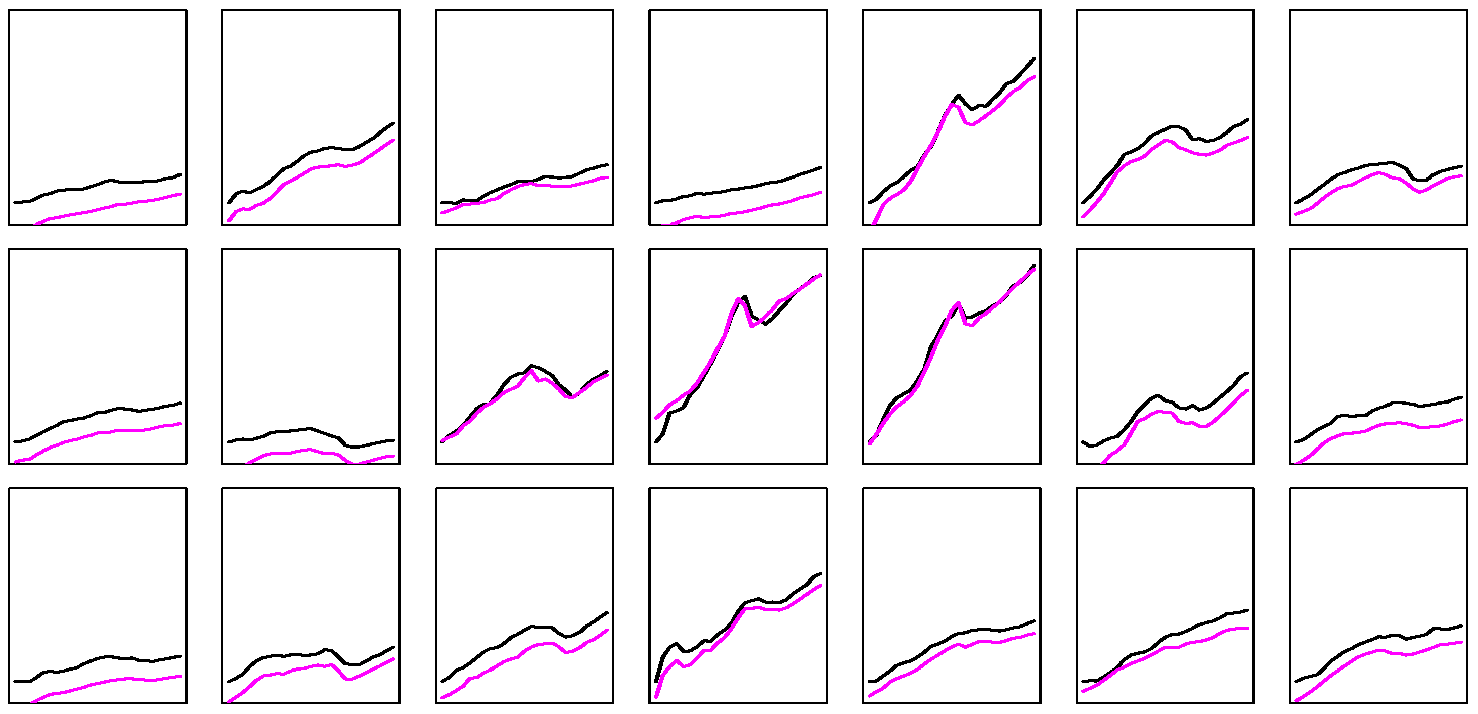
In order to find out a bit more about the strengths and weaknesses of our suggested procedure, we ran some prediction experiments based on simulated data. Because of the hierarchy of steps, such simulation experiments are time-consuming, so the number of replications remains limited. We simulate time-series data from basic time-series models, such as ARMA(1,1), and consider prediction based on ARMA(1,1) with coefficients estimated from the observations and also the simpler AR(1) model. The AR(1) model omits the MA(1) term of the generating model, but it may be competitive for small samples and for small MA coefficients.

We use a grid for the ARMA(1,1) model

$$X_t={\varphi }_0+\varphi X_{t-1}+{\epsilon }_t-\theta {\epsilon }_{t-1}$$

over $\varphi =-0.75,-0.5,\dots ,0.5,0.75$ and $\theta =-0.75,-0.5,\dots ,0.5,0.75$. The intercept ${\varphi }_0$ is always kept at zero, but all estimated models include an intercept term. We consider two distributions for the iid errors $\epsilon$, a standard $N(0,1)$ and a Cauchy distribution. The simulation-based strategy uses two variants. In the first variant, both the ARMA(1,1) and an AR(1) model are estimated from the data, and both estimated structures are simulated and again predicted based on both models. 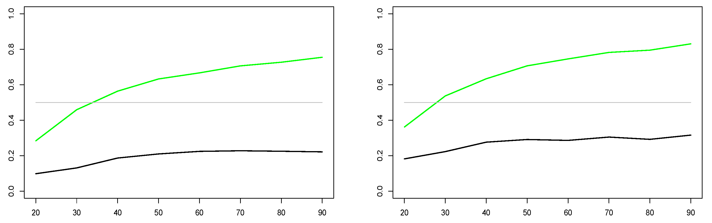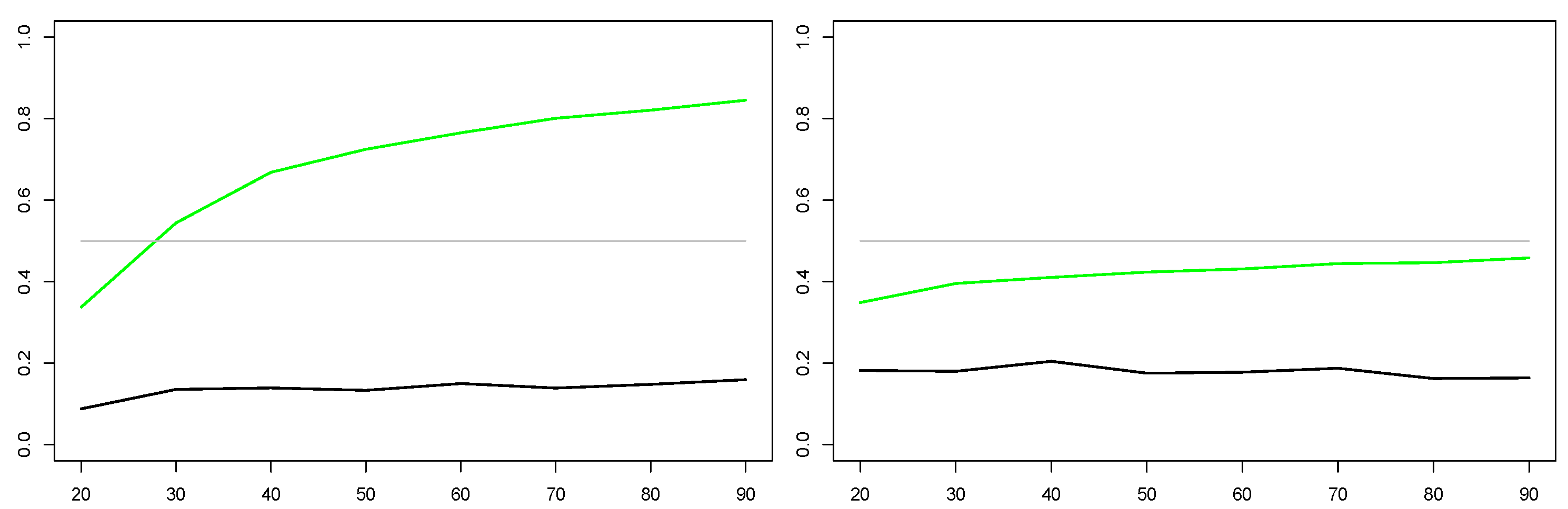This delivers four sub-experiments and, finally, the model—either AR(1) or ARMA(1,1)—is selected as a prediction model that more often defeats its ‘rival’ model. In the other variant, the mean squared forecast errors (MSFE) that evolve from both models are added up, and the model with the smaller average MSFE is selected. Forecasts from the thus selected models are then compared with the choice based on a classical AIC, an extremely competitive benchmark that is hard to beat. The experiments are summarized in Figure 1, which shows the optimum strategy for each combination of AR and MA coefficients, with an optimum defined as that strategy that ultimately yields the minimum (absolute) forecast error for the out-of-sample observation at position $t=N+1$. By construction, the diagonal connecting the southwest and the northeast corners represents white noise, as AR and MA terms cancel in $X_t={\varphi }_0+\varphi X_{t-1}+{\epsilon }_t-\varphi {\epsilon }_{t-1}$. The heterogeneity visible in the graphs reflects sampling variation.

For Gaussian errors, Figure 1 shows a preponderance of AIC-supporting cases for $T=50$ and $T=100$, whereas the contest is more open for $T=25$. Dominance is less explicit for Cauchy errors. From the two different evaluation methods for the simulation method, counting cases is preferable for most cases, so it may be interesting to reduce the rival strategies to two, the AIC and the simulation method with evaluating case counts. This design results in a quite similar figure, with almost all green dots turning blue. In summary, AIC appears invincible for large samples and Gaussian errors, whereas the simulator deserves consideration for small samples. This simulation experiment may be relevant for the empirical example to be studied in the next section, as the macroeconomic time-series sample remains in the lower region of the Monte Carlo evaluated in this section.

3. Data and Their Time-Series Properties

3.1. The Data

A full intrinsically homogeneous data set for household consumption and corresponding disposable income is not available from the Eurostat database, at least not for the majority of member countries. For this reason, we took the available information and constructed consumption and income series based on these support series. Even this reconstruction, however, was only feasible for a subset of countries, at least for the targeted full time range of 1995 to 2019 (annual data): Austria, Belgium, Cyprus, Czechia, Denmark, Estonia, Finland, France, Germany, Hungary, Ireland, Italy, Latvia, Lithuania, Netherlands, Poland, Slovakia, Slovenia, Spain, Sweden, and the United Kingdom. These are 21 countries that, for a considerable part of the time range, have been members of the European Union: some joined a bit later, whereas the United Kingdom left the EU recently. A visual summary of the consumption and income series is provided in Figure 2, where countries have been sorted in the EU tradition according to the beginning letters in the local languages. The full numerical data are available on request. Figure 2 shows that saving rates were almost always positive, which implies that households have been under some pressure during episodes of fiscal austerity but that aggregates were not often forced to dissave on a large scale. Of course, single households have been and are confronted with quite different situations. An exception to the rule are economies that were confronted with a fierce transition from a socialist to a market economy, such as the Baltic countries.

A similar heterogeneity can be seen regarding real income growth. The Eastern European economics have started from a much lower level and had to grow faster in order to catch up with Western Europe. It is known that this catching-up process was successful, and the Eastern spearheads such as Czechia have already overtaken the Western laggards such as Portugal. The distance between the two variables appears to be reasonably stable, and eyeballing would support cointegration.

Other disciplines may be surprised at the comparatively short time series that are routinely used by macroeconomists for their forecasts. Because of the deep transformation processes toward the end of the 20th century, longer series are not available for large parts of Europe. Forecasts based on such data sets represent an interesting challenge.

3.2. Time-Series Properties

The series at hand, 21 consumption and 21 income series, were subjected to unit-root tests with the alternative of stationarity. The series are rather short, and the unit-root tests have low power, so results are only summarily reported here. If one augmentation term is added to the basic Dickey–Fuller regression, which is the standard option in R, and a linear time trend is used in the regression, the tests fail to reject for any of the income series and reject only three times for the consumption series. Rejections are recorded for Belgium, France, and the Netherlands, i.e., three countries with some similarities and strong interaction. The time-series graphs, however, do not look very different from other countries, and the rejections may be caused by the smoothness of the curves that permits linear trends to approximate them particularly well, such that the remainder looks stationary. On the whole, it appears reasonable to proceed under the assumption of 42 first-order integrated (I(1)) variables.

If variables are I(1), they may be cointegrated. In modeling consumption and income, the research concentrates on the potential stationarity of the difference in logs between the variables, not on a freely estimated cointegrating vector. The economic motivation is that, for C and Y representing log consumption and income, respectively, any stationary variable of the form $C-Y^{\lambda }$ with $\lambda \ne 1$ would imply an unsustainable long-run relationship, with either consumption systematically exceeding income or a saving rate converging to zero. Figure 3 shows the calculated differences in a single plot. This graph intends to convey a general tendency, with country indicators—for example, the very high value for 1995 belongs to Latvia—deliberately suppressed. The summary visual evidence supports stationarity, but statistical Dickey–Fuller tests are less clear, rejecting the unit-root null only for five cases: Italy, Spain, and three more rather unrelated countries.

Figure 3 also gives an impression of convergence, as the cross-sample volatility appears to be stronger in the 1990s than toward the end of the sample. Such convergence would suggest assigning stronger weights to the late part of the sample or including a nonlinear, converging trend line. Within the limits of this paper, such extensions are ruled out and will be reserved for future work.

4. The Prediction Experiments

Assume a toolbox consisting of two models, a bivariate autoregression with cointegration and a bivariate autoregression in differences without cointegration. Furthermore, we are interested in whether the lag order of two that is recommended for most countries by most criteria is better than a lag order of three that is recommended only for relatively few countries. The two issues can be combined in the sense that cointegration can be studied with more or less lags in differences. Instinctively, we may conjecture that low-order models in differences yield poorer forecasts, as they process less information, and that they only forecast on par with their rivals when the restrictions are all valid, i.e., the parameters of concern are all zero.

It turns out, however, that this assumption is not generally confirmed in simulation experiments. Even if a structure with invalid zero restrictions has generated the data, it is quite often the case that simpler models outperform the ‘true’ models due to the fact that the entertained true models are not true literally, but they contain coefficient parameters that must be estimated from the data and necessarily involve some sampling variation. This effect has been well documented repeatedly in the forecasting literature (see, e.g., Kolassa, 2016, for the case of seasonality), although it still puzzles many researchers.

4.1. Models with and without Error Correction

This subsection reports our central experiment. Bivariate models with and without cointegration are fitted to the data. From the estimated parametric structures, pseudo-samples are generated. To these pseudo-data, again, both types of models, with and without error correction, are fitted. Finally, the performance of all four designs is comparatively evaluated.

We note that the seminal contribution by [15] did not consider a comparison between a cointegrating and a pure-difference model but, rather, between a cointegrating and a level autoregression, such that cointegration restricts the model. In practice, this comparison is less natural, as univariate time-series properties are easier to establish. For example, most researchers would agree that consumption and income series across Europe are better represented by first-order integrated than by stationary models. By contrast, whether and to what degree error correction affects collective behavior is less easy to establish statistically or to agree upon. We surmise that the choice taken by [15] was based on the correct observation that a model in differences is mis-specified if cointegration is present.

Figure 4 provides a graphical representation of the results from this experiment. The abscissa axis represents the available sample size, starting at the left with $T=20$, which roughly corresponds to the actual data from Eurostat. By contrast, the right end $T=90$ corresponds to the hypothetical situation with 90 years of available data whose dynamics are ‘similar’ to the observed Eurostat data. Indeed, the sample size of the pseudo-data proves to be a crucial determinant of relative performance. With $T=20$ and even $T=30$, the model without error correction dominates even when the generator model is cointegrating. This implies that inserting an error-correction term does not help in forecasting from small samples that are common in applications. For example, the European Monetary Union has a history of barely 20 years. For longer available data, cointegration helps if it is really present. Only for sample sizes beyond $T=60$ would it make sense to estimate an error-correction term even if there is a chance that it is spurious. It is a bit surprising that this second boundary appears to be at a slightly larger sample size for consumption, although traded wisdom has it that adjustment to the error correction is primarily performed by the consumption variable (the slave) rather than by the income variable (the master).

4.2. Longer Lags

The implications of lag specification are a traditional centerpiece of time-series model selection. It is well known that optimizing (i.e., minimizing) the AIC criterion due to [14] is tantamount to optimizing forecasting properties in large samples, but also that this strategy does not lead to consistency in the sense of capturing the true lag order as $T\to \infty$. In our panel, a lag order of two, i.e., a VAR(2), has been suggested by most criteria for most countries. In some countries, a lag order of one suffices, and for other countries, three is the recommended order.

In our simulation experiment, we consider first- and second-order vector autoregressions in differences, i.e.,

$$\Delta X_t={\mathsf{\Phi }}_0+{\mathsf{\Phi }}_1\Delta X_{t-1}+{\epsilon }_t$$

and

$$\Delta X_t={\mathsf{\Phi }}_0+{\mathsf{\Phi }}_1\Delta X_{t-1}+{\mathsf{\Phi }}_2\Delta X_{t-2}+{\epsilon }_t.$$

Both models are fitted to the data and then used to generate artificial pseudo-data. These pseudo-data are then forecast using both models. The outcome is summarized in Figure 5.

Figure 5 shows that larger lag orders are not promising for the income series at all. Even at $T=90$, D-VAR(1) remains the better forecaster than the ‘true’ D-VAR(2). Ninety years of macroeconomic data are unlikely to accumulate in the foreseeable future. In forecasting consumption, only 50–60 observations would be required to show an advantage for larger lag orders, even if the researcher is 50–50 undecided regarding whether such a lag order is needed.

5. Summary and Conclusions

We explore the technique of simulation-based forecast model selection in a panel data set of European income and consumption data. Variants of the time-series models are formulated, estimated, and simulated, and the relative merits of using each variant as a prediction tool are evaluated. The results confirm that statistical significance is an incomplete guideline for selecting forecasting models.

In detail, whereas the variables display noteworthy error-correction behavior, pure difference VAR models predict best in small samples, and they do so systematically. Similarly, the low lag order chosen for most individuals defines the best forecast model for quite large samples, at least for income, even if we allow for the possibility that a VAR with more lags has generated the sample.

The results not only contribute to the study of dynamic linkages among macroeconomic variables, they also demonstrate the power of the simulation-based selection procedure—it is simple and informative. More such examples will be considered in the future. In particular, it is to be noted that the symmetric approach does not face the usual difficulties in decisions between unit-root and stationary processes, a statistically non-standard problem that violates the regularity conditions of central limit theorems. Information criteria have been shown to be inadequate for this decision (see [16]). By contrast, the simulation-based approach faces no problem with this type of decision. Just like information criteria and in contrast to restriction tests, the approach is also readily applied to all non-nested decision situations.

We are planning to explore the properties of the method further, both in simulation studies based on artificial data and in empirically relevant applications.

References

1. Engle, R.F.; Granger, C.W.J. Co-Integration and Error Correction: Representation, Estimation, and Testing. Econometrica 1987, 55, 251–276. [Google Scholar] [CrossRef]
2. Han, H.L.; Ogaki, M. Consumption, income and cointegration. Int. Rev. Econ. Financ. 1997, 6, 107–117. [Google Scholar] [CrossRef]
3. Kunst, R.M.; Neusser, K. Cointegration in a Macroeconomic System. J. Appl. Econ. 1990, 5, 351–365. [Google Scholar] [CrossRef] [Green Version]
4. Jin, F. Cointegration of Consumption and Disposable Income: Evidence from Twelve OECD Countries. South. Econ. J. 1995, 62, 77–88. [Google Scholar] [CrossRef]
5. Ismail, A.; Rashid, K. Determinants of Household Saving: Cointegrated Evidence from Pakistan (1975–2011). Econ. Model. 2013, 32, 524–531. [Google Scholar] [CrossRef]
6. Klein, L.R.; Kosobud, R.F. Some Econometrics of Growth: Great Ratios of Economics. Q. J. Econ. 1961, 75, 173–198. [Google Scholar] [CrossRef]
7. Kunst, R.M. Cross validation of prediction models for seasonal time series by parametric bootstrapping. Austrian J. Stat. 2008, 37, 271–284. [Google Scholar]
8. Jumah, A.; Kunst, R.M. Seasonal prediction of European cereal prices: Good forecasts using bad models? J. Forecast. 2008, 27, 391–406. [Google Scholar] [CrossRef]
9. Granger, C.W.J. Investigating Causal Relations by Econometric Models and Cross-spectral Methods. Econometrica 1969, 37, 424–438. [Google Scholar] [CrossRef]
10. Giacomini, R.; White, H. Tests of Conditional Predictive Ability. Econometrica 2006, 74, 1545–1578. [Google Scholar] [CrossRef] [Green Version]
11. Kolassa, S. Sometimes It’s Better to Be Simple than Correct. Foresight 2016, 40, 20–26. [Google Scholar]
12. Jumah, A.; Kunst, R.M. Forecasting Agricultural Product and Energy Prices: A Simulation-Based Model Selection Approach; Institute for Advanced Studies: Vienna, Austria, 2018. [Google Scholar]
13. Peña, D.; Sanchez, I. Measuring the advantages of multivariate vs. univariate forecasts. J. Time Ser. Anal. 2007, 28, 886–909. [Google Scholar] [CrossRef]
14. Akaike, H. Statistical predictor identification. Ann. Inst. Stat. Math. 1970, 21, 243–247. [Google Scholar] [CrossRef]
15. Engle, R.F.; Yoo, B.S. Forecasting and testing in co-integrated systems. J. Econom. 1987, 35, 143–159. [Google Scholar] [CrossRef]
16. Phillips, P.C.B.; Ploberger, W. Empirical Limits for Time Series Econometric Models. Econometrica 2003, 71, 627–673. [Google Scholar]
Figure 1. Best selection strategy for forecasting simulated ARMA(1,1) data. ARMA(1,1) models are generated with T = 25 , 50 , 100 . Upper row N ( 0 , 1 ) errors, lower row Cauchy errors. ϕ = 0.75 , 0.5 , , 0.75 on the x-axis and θ = 0.75 , 0.5 , , 0.75 on the y-axis. Red denotes AIC, green MSE simulator, blue counting simulator.
Engproc 05 00055 g001
Figure 2. Eurostat data for household consumption (pink) and aggregate disposable income (black) for the following countries: Belgium, Czechia, Denmark, Germany, Estonia, Ireland, Spain, France, Italy, Cyprus, Latvia, Lithuania, Hungary, Netherlands, Austria, Poland, Slovenia, Slovakia, Finland, Sweden, United Kingdom.
Engproc 05 00055 g002
Figure 3. Log consumption minus log income for 21 countries.
Engproc 05 00055 g003
Figure 4. Percentage of error-correction models yielding the better forecast for consumption (left) and income (right). Green curve for cointegrated generators, black curve for non-cointegrated generators.
Engproc 05 00055 g004
Figure 5. Percentage of VAR(2) models in differences yielding the better forecast for consumption (left) and income (right). Green curve for VAR(2) generators, black curve for VAR(1) generators.
Engproc 05 00055 g005
Publisher’s Note: MDPI stays neutral with regard to jurisdictional claims in published maps and institutional affiliations.