Semiparametric Block Bootstrap Prediction Intervals for Parsimonious Autoregression ^†

Abstract

This paper investigates the research question of whether the principle of parsimony carries over into interval forecasting, and proposes new semiparametric prediction intervals that apply the block bootstrap to the first-order autoregression. The AR(1) model is parsimonious in which the error term may be serially correlated. Then, the block bootstrap is utilized to resample blocks of consecutive observations to account for the serial correlation. The Monte Carlo simulations illustrate that, in general, the proposed prediction intervals outperform the traditional bootstrap intervals based on nonparsimonious models.

1. Introduction

It is well known that a parsimonious model may produce superior out-of-sample point forecasts compared to a complex model with overfitting issue, see [1]. One objective of this paper is to examine whether the principle of parsimony (POP) can be extended to interval forecasts. Toward that end, this paper proposes a semiparametric block bootstrap prediction intervals (BBPI) based on a parsimonious first-order autoregression AR(1). By contrast, the standard or iid bootstrap prediction intervals developed by Thombs and Schucany [2] (called TS intervals thereafter) are based on a dynamically adequate AR(p), where p can be large.

A possibly overlooked fact is that there is inconsistency between the ways of obtaining point forecasts and interval forecasts, in terms of whether POP is applied. When the goal is the point forecast, the models selected by information criteria of AIC and BIC are typically parsimonious, but not necessarily adequate (see Enders Enders [3] for instance). However, POP is largely forgone by the classical Box–Jenkins prediction intervals and the TS intervals; both require serially uncorrelated error terms, and the chosen models can be very complicated.

This paper attempts to address that inconsistency. The key is to note that the essence of time series forecasting is to utilize the serial correlation, and there are multiple ways to do that. One way is to use a dynamically adequate AR(p) with serially uncorrelated errors, which is fully parametric. This paper instead employs a parsimonious AR(1) with possibly serially correlated errors. Our model is semiparametric since no specific function form is assumed for the error process. Our semiparametric approach of leaving some degree of serial correlation in the error term is similar to the famous Cochrane–Orcutt procedure of Cochrane and Orcutt [4].

We employ the AR(1) model in order to generate the bootstrap replicate. In particular, we are not interested in the autoregressive coefficient, and for our purposes, it becomes irrelevant that the OLS estimate may be inconsistent due to the autocorrelated error. Using the AR(1) has another advantage: the likelihood of multicollinearity is minimized, which can result in a more efficient estimate for the coefficient. On the other hand, we do want to make use of the correlation structure in the error, and that is fulfilled by using the block bootstrap. More explicitly, the block bootstrap redraws with replacement random blocks of consecutive residuals of the AR(1). The blocking is intended to preserve the time dependence structure.

Constructing the BBPI involves three steps. In step one, the AR(1) regression is estimated by ordinary least squares (OLS), and the residual is saved. In step two, a backward AR(1) regression is fitted, and random blocks of residuals are used to generate the bootstrap replicate. In step three the bootstrap replicate is used to run the AR(1) regression again and random blocks of residuals are used to compute the bootstrap out-of-sample forecast. After repeating steps two and three many times, the BBPI is determined by the percentiles of the empirical distribution of the bootstrap forecast (In the full-length version of the paper, which is available upon request, we discuss technical issues such as correcting the bias of autoregressive coefficients, selecting the block size, choosing between overlapping and non-overlapping blocks, and using the stationary bootstrap developed by Politis and Romano [5]).

We implement the Monte Carlo experiment that compares the average coverage rate of the BBPI to the TS intervals. There are two main findings. The first is that the BBPI dominates when the error term shows a strong serial correlation. The second is that the BBPI always outperforms the TS intervals for the one-step forecast. For a longer forecast horizon, the TS intervals may perform better. This second finding highlights a tradeoff between preserving correlation and adding variation when obtaining the bootstrap intervals. The block bootstrap achieves the former but sacrifices the latter.

There is a growing body of literature on the bootstrap prediction intervals. Important works include Thombs and Schucany [2], Masarotto [6], Grigoletto [7], Clements and Taylor [8], Kim [9], Kim [10], Staszewska-Bystrova [11], Fresoli et al. [12], and Li [13]. The block bootstrap is developed by Künsch [14]. This work distinguishes itself by applying the block bootstrap to interval forecasts based on univariate AR models. The remainder of the paper is organized as follows. Section 2 specifies the BBPI. Section 3 conducts the Monte Carlo experiment. Section 4 concludes.

2. Semiparametric Block Bootstrap Prediction Intervals

Let $\left\{y_t\right\}$ be a strictly stationary and weakly dependent time series with mean of zero. In practice, $y_t$ may represent the demeaned, differenced, detrended or deseasonalized series. At first, it is instructive to emphasize a fact: there are multiple ways to model a time series. For instance, suppose the data generating process (DGP) is an AR(2) with serially uncorrelated errors:

$$y_t={\varphi }_1{y}_{t-1}+{\varphi }_2{y}_{t-2}+e_t,$$

(1)

where $e_t$ can be white noise or martingale difference. Then, we can always rewrite Equation (1) as an AR(1) with new error $v_t,$ and the new error follows an AR(1) process, so is serially correlated:

$$\begin{array}{ccc}\hfill y_t& =& \varphi y_{t-1}+v_t\hfill \end{array}$$

(2)

$$\begin{array}{ccc}\hfill v_t& =& \rho v_{t-1}+e_t\hfill \end{array}$$

(3)

where ${\varphi }_1=\rho +\varphi$ and ${\varphi }_2=-\rho \varphi$ by construction. The point is, the exact form of the DGP does not matter. In this example, it can be AR(1) or AR(2). What matters is the serial correlation of $y_t,$ which can be captured by Equation (1), or Equation (2) along with Equation (3) equally well. This example indicates that it is plausible to obtain forecasts based on the parsimonious AR(1) model, as long as the serial correlation in $v_t$ has been accounted for, even if the “true” DGP is a general AR(p).

There is concern that the estimated coefficient of $\widehat{\varphi }$ in Equation (2) will be inconsistent due to the autocorrelated error $v_t.$ However, this issue is largely irrelevant here because our focal point is forecasting $y,$ not estimating the coefficient. One may use the generalized least squares method such as Cochrane–Orcutt estimation to mitigate the effect of serial correlation bias. Our Monte Carlo experiment shows that the proposed intervals perform well even without correcting the serial correlation bias.

Using the parsimonious model (2) has two benefits that are overlooked in the forecasting literature. First, notice that $y_{t-1}$ is correlated with $y_{t-2}.$ As a result, there is the issue of multicollinearity (correlated regressors) for Equation (1), but not Equation (2). The absence of multicollinearity can reduce the variance and improve the efficiency of $\widehat{\varphi },$ which explains why a simple model can outperform a complicated model in terms of out-of-sample forecasting. Second, it is well known that the autoregressive coefficient estimated by OLS can be biased—see Shaman and Stine [15], for instance. As more coefficients need to be estimated in a complex AR model, its forecast can be less accurate than that of a parsimonious model.

2.1. Iterated Block Bootstrap Prediction Intervals

The goal is to find the prediction intervals for future values $(y_{n+1},y_{n+2},\dots ,y_{n+h}),$ where h is the maximum forecast horizon, after observing $\Omega =(y_1,\dots ,y_n).$ This paper focuses on the bootstrap prediction intervals because (i) they do not assume the distribution of $y_{n+i}$ conditional on $\Omega$ is normal, and (ii) the bootstrap intervals can automatically take into account the sampling variability of the estimated coefficients.

The TS intervals of Thombs and Schucany [2] are based on a “long” p-th order autoregression:

$$y_t={\psi }_1{y}_{t-1}+{\psi }_2{y}_{t-2}+\dots +{\psi }_p{y}_{t-p}+e_t.$$

(4)

The TS intervals assume that the error $e_t$ is serially uncorrelated, because the standard or iid bootstrap only works in the independent setting. This assumption of independent errors requires that the model (4) be dynamically adequate, i.e., a sufficient number of lagged values should be included. It is not uncommon that the chosen model can be complicated (e.g., for series with a long memory), which contradicts the principle of parsimony.

Actually, the model (4) is just a finite-order approximation if the true DGP is an ARMA process with AR$(\infty )$ representation. In that case, the error $e_t$ is always serially correlated no matter how large p is. This extreme case implies that the assumption of serially uncorrelated errors can be too restrictive in practice.

This paper relaxes that independence assumption, and proposes the block bootstrap prediction intervals (BBPI) based on a “short” autoregression. Consider the AR(1), the simplest one:

$$y_t={\varphi }_1{y}_{t-1}+v_t.$$

(5)

Most often, the error $v_t$ is serially correlated, so model (5) is inadequate. Nevertheless, the serial correlation in $v_t$ can be utilized to improve the forecast. Toward that end, the block bootstrap will later be applied to the residual

$${\widehat{v}}_t=y_t-{\widehat{\varphi }}_1{y}_{t-1},$$

(6)

where ${\widehat{\varphi }}_1$ is the coefficient estimated by OLS.

But first, any bootstrap prediction intervals should account for the sampling variability of ${\widehat{\varphi }}_1.$ This is accomplished by running repeatedly the regression (5) using the bootstrap replicate, a pseudo time series. Following Thombs and Schucany [2] we generate the bootstrap replicate using the backward representation of the AR(1) model

$$y_t={\theta }_1{y}_{t+1}+u_t.$$

(7)

Note that the regressor is lead not lag. Denote the OLS estimate by ${\widehat{\theta }}_1,$ and the residual by ${\widehat{u}}_t:$

$${\widehat{u}}_t=y_t-{\widehat{\theta }}_1{y}_{t+1},$$

(8)

then one series of the bootstrap replicate $(y_1^{\ast },\dots ,y_n^{\ast })$ is computed in a backward fashion as (starting with the last observation, then moving backward)

$$y_n^{\ast }=y_n,y_t^{\ast }={\widehat{\theta }}_1{y}_{t+1}^{\ast }+{\widehat{u}}_t^{\ast },(t=n-1,\dots 1).$$

(9)

By using the backward representation we can ensure the conditionality of AR forecasts on the last observed value $y_n.$ Put differently, all the bootstrap replicate series have the same last observation, $y_n^{\ast }=y_n.$ See Figure 1 of Thombs and Schucany [2] for an illustration of this conditionality.

In Equation (9), the randomness of the bootstrap replicate comes from the pseudo error term ${\widehat{u}}_t^{\ast },$ which is obtained by the block bootstrap as follows:

• Save the residual of the backward regression ${\widehat{u}}_t$ given in Equation (8).
• Let b denote the block size (length). The first (random) block of residuals is

  $$B_1=({\widehat{u}}_{i1},{\widehat{u}}_{i1+1},\dots ,{\widehat{u}}_{i1+b-1}),$$

  (10)

  where the index number $i1$ is a random draw from the discrete uniform distribution between 1 and $n-b+1.$ For instance, let $b=3$ and suppose a random draw produces $i1=20,$ then $B_1=({\widehat{u}}_{20},{\widehat{u}}_{21},{\widehat{u}}_{22}).$ In this example the first block contains three consecutive residuals starting from the 20th observation. By redrawing the index number with replacement we can obtain the second block $B_2=({\widehat{u}}_{i2},{\widehat{u}}_{i2+1},\dots ,{\widehat{u}}_{i2+b-1}),$ the third block $B_3=({\widehat{u}}_{i3},{\widehat{u}}_{i3+1},\dots ,{\widehat{u}}_{i3+b-1}),$ and so on. We stack up these blocks until the length of the stacked series becomes $n.$${\widehat{u}}_t^{\ast }$ denotes the t-th observation of the stacked series.

Resampling blocks of residuals is intended to preserve the serial correlation of the error term in the parsimonious model. Generally speaking, the block bootstrap can be applied to any weakly dependent stationary series. Here it is applied to the residual of the short autoregression.

After generating the bootstrap replicate series using Equation (9), next, we refit the model (5) using the bootstrap replicate $(y_2^{\ast },\dots ,y_n^{\ast }).$ Denote the newly estimated coefficient (called bootstrap coefficient) by ${\widehat{\varphi }}_1^{\ast }.$ Then, we can compute the iterated block bootstrap l-step forecast ${\widehat{y}}_{n+l}^{\ast }$ as

$${\widehat{y}}_n^{\ast }=y_n,{\widehat{y}}_{n+l}^{\ast }={\widehat{\varphi }}_1^{\ast }{\widehat{y}}_{n+l-1}^{\ast }+{\widehat{v}}_l^{\ast },(l=1,\dots ,h)$$

(11)

where the pseudo error ${\widehat{v}}_l^{\ast }$ is obtained by block bootstrapping the residual (6). For example, let $h=8,b=4.$ Then two blocks of residuals (6) are randomly drawn, and they are $B_1=({\widehat{v}}_{i1},{\widehat{v}}_{i1+1},{\widehat{v}}_{i1+2},{\widehat{v}}_{i1+3}),$$B_2=({\widehat{v}}_{i2},{\widehat{v}}_{i2+1},{\widehat{v}}_{i2+2},{\widehat{v}}_{i2+3}).$ Notice that ${\widehat{v}}_l^{\ast }$ in Equation (11) represents the l-th observation of the stacked series

$${\left\{{\widehat{v}}_l^{\ast }\right\}}_{l=1}^h=\{{\widehat{v}}_{i1},{\widehat{v}}_{i1+1},{\widehat{v}}_{i1+2},{\widehat{v}}_{i1+3},{\widehat{v}}_{i2},{\widehat{v}}_{i2+1},{\widehat{v}}_{i2+2},{\widehat{v}}_{i2+3}\}.$$

(12)

The ordering of $B_1$ and $B_2$ in the stacked series (12) does not matter. It is the ordering of the observations within each block that matters. That within-block ordering preserves the temporal structure.

Notice that the block bootstrap has been invoked twice: first it is applied to ${\widehat{u}}_t$ (8), then it is applied to ${\widehat{v}}_t$ (6). The first application adds randomness to the bootstrap replicate $y_t^{\ast };$ whereas the second application randomizes the predicted value ${\widehat{y}}_{n+l}^{\ast }.$

To get the BBPI, we need to generate C series of the bootstrap replicate (9), use them to fit the model (5), and use Equation (11) to obtain a series of the iterated block bootstrap l-step forecasts

$${\left\{{\widehat{y}}_{n+l}^{\ast }\left(i\right)\right\}}_{i=1}^C$$

(13)

where i is the index. The l-step iterated BBPI at the $\alpha$ nominal level are given by

$$l-\mathtt{step}\mathtt{Iterated}\mathtt{BBPI}\left(\mathtt{IBBPI}\right)=\left[{\widehat{y}}_{n+l}^{\ast }\left(\frac{1-\alpha }{2}\right),{\widehat{y}}_{n+l}^{\ast }\left(\frac{1+\alpha }{2}\right)\right]$$

(14)

where ${\widehat{y}}_{n+l}^{\ast }\left(\frac{1-\alpha }{2}\right)$ and ${\widehat{y}}_{n+l}^{\ast }\left(\frac{1+\alpha }{2}\right)$ are the $\left(\frac{1-\alpha }{2}\right)100$-th and $\left(\frac{1+\alpha }{2}\right)100$-th percentiles of the empirical distribution of ${\left\{{\widehat{y}}_{n+l}^{\ast }\left(i\right)\right\}}_{i=1}^C.$ Throughout this paper, we let $\alpha =0.90.$ To avoid the discreteness problem, one may let $C=999,$ see Booth and Hall [16]. In this paper we use $C=1000$ and find no qualitative difference.

Basically, we apply the percentile method of Efron and Tibshirani [17] to construct the BBPI. De Gooijer and Kumar [18] emphasize the percentile method performs well when the conditional distribution of the predicted values is unimodal. In preliminary simulation, we conduct the DIP test of Hartigan and Hartigan [19] and find that the distribution is indeed unimodal.

2.2. Direct Block Bootstrap Prediction Intervals

We call the BBPI (14) iterated because the forecast is computed in an iterative fashion: in Equation (11), the previous step forecast ${\widehat{y}}_{n+l-1}^{\ast }$ is used to compute the next step ${\widehat{y}}_{n+l}^{\ast }.$ Alternatively, we can use the bootstrap replicate $(y_1^{\ast },\dots ,y_n^{\ast })$ to run a set of direct regressions using only one regressor. In total there are h direct regressions. More explicitly, the l-th direct regression uses $y_t^{\ast }$ as the dependent variable and $y_{t-l}^{\ast }$ as the independent variable. Denote the estimated direct coefficient by ${\widehat{\rho }}_l^{\ast }.$ The residual is computed as

$${\widehat{\eta }}_{t,l}=y_t^{\ast }-{\widehat{\rho }}_l^{\ast }{y}_{t-l}^{\ast }.$$

(15)

Then, the direct bootstrap forecast is computed as

$${\widehat{y}}_{n+l}^{d\ast }={\widehat{\rho }}_l^{\ast }{y}_n+{\widehat{\eta }}_l^{\ast }$$

(16)

where ${\widehat{\eta }}_l^{\ast }$ is a random draw with replacement from the empirical distribution of ${\widehat{\eta }}_{t,l}.$ The l-step direct BBPI at the $\alpha$ nominal level is given by

$$l-\mathtt{step}\mathtt{Direct}\mathtt{BBPI}\left(\mathtt{DBBPI}\right)=\left[{\widehat{y}}_{n+l}^{d\ast }\left(\frac{1-\alpha }{2}\right),{\widehat{y}}_{n+l}^{d\ast }\left(\frac{1+\alpha }{2}\right)\right]$$

(17)

where ${\widehat{y}}_{n+l}^{d\ast }\left(\frac{1-\alpha }{2}\right)$ and ${\widehat{y}}_{n+l}^{d\ast }\left(\frac{1+\alpha }{2}\right)$ are the $\left(\frac{1-\alpha }{2}\right)100$-th and $\left(\frac{1+\alpha }{2}\right)100$-th percentiles of the empirical distribution of ${\left\{{\widehat{y}}_{n+l}^{d\ast }\left(i\right)\right\}}_{i=1}^C.$

There are other ways to obtain the direct prediction intervals. For example, the bootstrap replicate $(y_1^{\ast },\dots ,y_n^{\ast })$ can be generated based on the backward form of direct regression. Ing [20] compares the mean-squared prediction errors of the iterated and direct point forecasts. In the next section, we will compare the iterated and direct BBPIs.

3. Monte Carlo Experiment

3.1. Error Distributions

This section compares the performances of various bootstrap prediction intervals using the Monte Carlo experiment. First, we investigate the distribution of error terms. Following Thombs and Schucany [2], the data generating process (DGP) is an AR(2):

$$y_t={\varphi }_1{y}_{t-1}+{\varphi }_2{y}_{t-2}+u_t$$

(18)

where ${\varphi }_1=0.75,{\varphi }_2=-0.5,$$t=1,\dots ,55.$ The error $u_t$ follows an independently and identically distributed process. Three distributions are considered for $u_t$: the standard normal distribution, the exponential distribution with mean of 0.5, and mixed normal distribution $0.9N(-1,1)+0.1N(9,1).$ The exponential distribution is skewed; the mixed normal distribution is bimodal and skewed. All distributions are centered to have zero mean.

We compare three bootstrap prediction intervals. The iterated block bootstrap prediction intervals (IBBPI) are based on the “short” AR(1) regression (5) and its backward form (7). The TS intervals of Thombs and Schucany [2] are based on the “long” AR(2) regression (18) and its backward form. Finally, the direct block bootstrap prediction intervals (DBBPI) are based on a series of first-order direct autoregressions. Each bootstrap prediction intervals are obtained from the empirical distribution of 1000 bootstrap forecasts. That is, we let $C=1000$ in Equation (13) for the IBBPI, and so on. For the IBBPI and DBBPI, the block size b is 4. The TS intervals use the iid bootstrap, so $b=1.$

The first 50 observations $(n=50)$ are used to fit the regression. Then, we evaluate whether the last five observations are inside the prediction intervals. That is, we focus on the out-of-sample forecasting. The main criterion for comparison is the average coverage rate (ACR):

$$\mathtt{ACR}\left(h\right)=m^{-1}\sum _{i=1}^{m}1(y_{n+h}\in \mathtt{Prediction}\mathtt{Intervals})$$

(19)

where $1(.)$ denotes the indicator function. The number of iteration is set as m = 20,000. The forecast horizon h ranges from 1 to 5. The nominal coverage $\alpha$ is 0.90. The intervals whose ACR is closest to 0.90 are deemed the best.

Figure 1 plots the ACR against $h,$ in which the ACRs of the IBBPI, TS intervals, and DBBPI are denoted by circle, square and star, respectively. In the leftmost graph, the error follows the standard normal distribution. It is shown that the ACR of the IBBPI is closest to the nominal coverage 0.90, followed by the TS intervals. The DBBPI have the worst performance. For instance, when $h=5,$ the IBBPI has ACR of 0.883, the TS intervals have ACR of 0.854, and the DBBPI has ACR of 0.829.

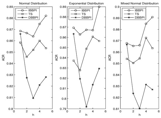
Figure 1. Error Distributions.

The ranking remains largely unchanged for the exponential distribution (in the middle graph) and mixed normal distribution (in the rightmost graph). Overall, Figure 1 indicates that (i) the IBBPI has the best performance, and (ii) the DBBPI has the worst performance. Finding (ii) complements Ing [20], which shows that the iterated point forecast outperforms the direct point forecast. Finding (i) is new. By comparing the three graphs in Figure 1, we see no significant change in ACRs as the error distribution varies. This is expected because all intervals are bootstrap intervals that do not assume normality.

3.2. Autoregressive Coefficients

Now, we consider varying autoregressive coefficients in Equation (18):

$$\begin{array}{ccc}& & {\varphi }_1=0.75,{\varphi }_2=-0.5\left(\mathtt{stationary}\mathtt{AR}\left(\mathtt{2}\right)\right)\hfill \end{array}$$

(20)

$$\begin{array}{ccc}& & {\varphi }_1=1.0,{\varphi }_2=-0.24\left(\mathtt{stationary}\mathtt{AR}\left(\mathtt{2}\right)\right)\hfill \end{array}$$

(21)

$$\begin{array}{ccc}& & {\varphi }_1=1.2,{\varphi }_2=-0.2(\mathtt{non}-\mathtt{stationary}\mathtt{AR}\left(\mathtt{2}\right))\hfill \end{array}$$

(22)

where $t=1,\dots ,55$ and $u_t\sim \mathtt{iidn}(0,1).$ The leftmost graph in Figure 2 looks similar to that in Figure 1 because the same DGP is used. In the middle graph we see no change in the ranking. The rightmost graph is interesting, where the sum of autoregressive coefficients is $1.2-0.2=1.$ Therefore, the series becomes nonstationary (having unit root). Obviously, nonstationarity causes distortion in the coverage rate, particularly when h is large. In light of this, we recommend applying the prediction intervals to the differenced data if unit roots are present. It is surprising to see the direct intervals are the best in the presence of nonstationarity, which may be explained by the fact that they are based on the direct regression (More simulations can be found in the full-length version of the paper where we examine the effects of sample sizes and sizes of blocks, and we compare block bootstrap intervals vs stationary bootstrap intervals, and overlapping vs non-overlapping blocks).

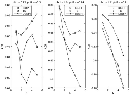
Figure 2. Autoregressive Coefficients.

3.3. Principle of Parsimony

So far the DGP has been the AR(2). Next we use an ARMA(1,1) as the new DGP:

$$y_t=\varphi y_{t-1}+u_t+\theta u_{t-1}$$

(23)

where $t=1,\dots ,55$ and $u_t\sim \mathtt{iidn}(0,1).$ In theory, there is AR$(\infty )$ representation for this DGP. Thus, any AR(p) model is a finite-order approximation.

We verify the principle of parsimony (POP) in two ways. Figure 3 compares the iterated block bootstrap prediction intervals based on the AR(1) regression, to the TS intervals based on the AR(2) regression (TS2, denoted by diamond), the AR(3) regression (TS3, denoted by square) and the AR(4) regression (TS4, denoted by star). For the TS intervals, we do not check whether the residual is serially uncorrelated. That job is left to Figure 4.

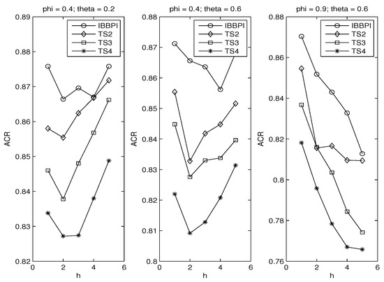
Figure 3. Parsimony I.

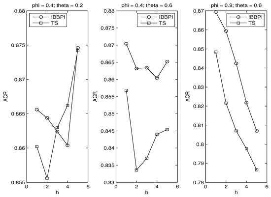
Figure 4. Parsimony II.

Figure 3 uses three sets of $\varphi$ and $\theta .$ We see the block bootstrap intervals have the best performance in all cases. The performance of the TS deteriorates as the autoregression gets longer. This is the first evidence that POP may be applicable for interval forecasts.

The second evidence is presented in Figure 4, where the TS intervals are based on the autoregression whose order is determined by the Breusch–Godfrey test, which is appropriate since the regressors are lagged dependent variables (so the regressors are not strictly exogenous). This is how the model selection works. We start from the AR(1) regression. If the residual passes the Breusch–Godfrey test, then the AR(1) regression is chosen for constructing the TS intervals. Otherwise, we move to the AR(2) regression, apply the Breusch–Godfrey test again, and so on. In the end, the TS intervals are based on an adequate autoregression with serially uncorrelated errors.

In the leftmost graph of Figure 4, $\varphi =0.4,\theta =0.2.$ We see the BBPI outperforms the TS intervals when h equals 1 and 2; for higher h their ranking reverses. In the middle and rightmost graphs, more serial correlation is induced as $\theta$ rises from 0.2 to 0.6, and as $\varphi$ rises from 0.4 to 0.9. In those two graphs, the BBPI dominates the TS intervals.

The fact that the BBPI fails to dominate the TS intervals in the leftmost graph indicates a tradeoff between preserving serial correlation and adding variation. Remember that the BBPI uses the block bootstrap that emphasizes preserving serial correlation. By contrast, the TS intervals use the iid bootstrap, which can generate more variation in the bootstrap replicate than the block bootstrap.

Keeping that in mind, then the leftmost graph makes sense. In that graph, $\theta$ is 0.2, close to zero. That means the ARMA(1,1) model is essentially an AR(1) model with weakly correlated errors. For such series preserving correlation becomes secondary.

Therefore, the TS intervals may perform better than the BBPI in the presence of weakly correlated errors. It is instructive to consider the limit, when the serial correlation becomes 0 and the error term becomes serially uncorrelated. Then, the block size should reduce to 1, and the block bootstrap degenerates to the iid bootstrap, which works best in the independent setting.

Finally, from Figure 3 and Figure 4 we notice that when $h=1,$ the BBPI always outperforms the TS intervals, no matter the serial correlation is weak or strong. This fact adds value to the BBPI for the short-horizon forecasts.

4. Conclusions

This paper proposes new prediction intervals by applying the block bootstrap to the first-order autoregression. The AR(1) model is parsimonious in which the error term can be serially correlated. Then, the block bootstrap is utilized to resample blocks of consecutive observations in order to maintain the time series structure of the error term. The forecasts can be obtained in an iterated manner, or by running direct regressions. The Monte Carlo experiment shows (1) there is evidence that the principle of parsimony can be extended to interval forecast; (2) there is a trade-off between preserving correlation and adding variation; (3) the proposed intervals have superior performance for one-step forecast.

References

- James, G.; Witten, D.; Hastie, T.; Tibshirani, R. An Introduction to Statistical Learning: With Applications in R; Springer: Berlin/Heidelberg, Germany, 2013. [Google Scholar]
- Thombs, L.A.; Schucany, W.R. Bootstrap prediction intervals for autoregression. J. Am. Stat. Assoc. 1990, 85, 486–492. [Google Scholar] [CrossRef]
- Enders, W. Applied Econometric Times Series, 3rd ed.; Wiley: Hoboken, NJ, USA, 2009. [Google Scholar]
- Cochrane, D.; Orcutt, G.H. Application of least squares regression to relationships containing auto-correlated error terms. J. Am. Stat. Assoc. 1949, 44, 32–61. [Google Scholar]
- Politis, D.N.; Romano, J.P. The Stationary Bootstrap. J. Am. Stat. Assoc. 1994, 89, 1303–1313. [Google Scholar] [CrossRef]
- Masarotto, G. Bootstrap prediction intervals for autoregressions. Int. J. Forecast. 1990, 6, 229–239. [Google Scholar] [CrossRef]
- Grigoletto, M. Bootstrap prediction intervals for autoregressions: Some alternatives. Int. J. Forecast. 1998, 14, 447–456. [Google Scholar] [CrossRef]
- Clements, M.P.; Taylor, N. Boostrapping prediction intervals for autoregressive models. Int. J. Forecast. 2001, 17, 247–267. [Google Scholar] [CrossRef]
- Kim, J. Bootstrap-after-bootstrap prediction intervals for autoregressive models. J. Bus. Econ. Stat. 2001, 19, 117–128. [Google Scholar] [CrossRef]
- Kim, J. Bootstrap prediction intervals for autoregressive models of unknown or infinite lag order. J. Forecast. 2002, 21, 265–280. [Google Scholar] [CrossRef]
- Staszewska-Bystrova, A. Bootstrap prediction bands for forecast paths from vector autoregressive models. J. Forecast. 2011, 30, 721–735. [Google Scholar] [CrossRef]
- Fresoli, D.; Ruiz, E.; Pascual, L. Bootstrap multi-step forecasts of non-Gaussian VAR models. Int. J. Forecast. 2015, 31, 834–848. [Google Scholar] [CrossRef] [Green Version]
- Li, J. Block Bootstrap Prediction Intervals for Parsimonious First-Order Vector Autoregression. J. Forecast. 2021, 40, 512–527. [Google Scholar] [CrossRef]
- Künsch, H.R. The Jackknife and the Bootstrap for General Stationary Observations. Ann. Stat. 1989, 17, 1217–1241. [Google Scholar] [CrossRef]
- Shaman, P.; Stine, R.A. The bias of autoregressive coefficient estimators. J. Am. Stat. Assoc. 1988, 83, 842–848. [Google Scholar] [CrossRef]
- Booth, J.G.; Hall, P. Monte Carlo approximation and the iterated bootstrap. Biometrika 1994, 81, 331–340. [Google Scholar] [CrossRef]
- Efron, B.; Tibshirani, R.J. An Introduction to the Bootstrap; Chapman and Hall: London, UK, 1993. [Google Scholar]
- De Gooijer, J.G.; Kumar, K. Some recent developments in non-linear time series modeling, testing, and forecasting. Int. J. Forecast. 1992, 8, 135–156. [Google Scholar] [CrossRef]
- Hartigan, J.A.; Hartigan, P.M. The DIP test of unimodality. Ann. Stat. 1985, 13, 70–84. [Google Scholar] [CrossRef]
- Ing, C.K. Multistep Prediction in Autogressive Processes. Econom. Theory 2003, 19, 254–279. [Google Scholar] [CrossRef] [Green Version]
Publisher’s Note: MDPI stays neutral with regard to jurisdictional claims in published maps and institutional affiliations. |
© 2021 by the author. Licensee MDPI, Basel, Switzerland. This article is an open access article distributed under the terms and conditions of the Creative Commons Attribution (CC BY) license (https://creativecommons.org/licenses/by/4.0/).