Comparative Analysis of Statistical and Analytical Techniques for the Study of GNSS Geodetic Time Series ^†

Abstract

GNSS systems allow precise resolution of the geodetic positioning problem through advanced techniques of GNSS observation processing (PPP or relative positioning). Current instrumentation and communications capabilities allow obtaining geocentric and topocentric geodetic high frequencies time series, whose analysis provides knowledge of the tectonic or volcanic geodynamic activity of a region. In this work, the GNSS time series study was carried out through the use and adaptation of R packets to determine their behavior, obtaining displacement velocities, noise levels, precursors in the time series, anomalous episodes, and their temporal forecast. Statistical and analytical methods were studied, for example, ARMA, ARIMA models, least-squares methods, wavelet functions, and Kalman techniques. To carry out a comparative analysis of these techniques and methods, significant GNSS time series obtained in geodynamically active regions (tectonic and/or volcanic) were considered.

1. Introduction

GNSS systems (GPS—USA, Glonass—Russia, Galileo—European Union, and Beidou—China), initially designed for land, sea, and air navigation, possess the ability to use specific and advanced techniques and methods to provide precisions sufficient to evaluate the movement of tectonic plates, the volcanic activity, or possible hillside landslides from the velocities obtained in positioning successive subcentimeter precision.

Geodynamic GNSS geodetic networks are based on permanent stations that operate continuously, even for high sample rates. The positions obtained make up time series, initially in geocentric Cartesian coordinates $(X,Y,Z)$. To facilitate the notion of displacement on the surface of the Earth, these coordinates are transformed into a topocentric system $(e,n,u)$. The analysis of these series provides the displacement velocity vector as well as the anomalies that may have occurred in the time period defined by the series. For this, and according to the objective of the study, different analytical or statistical methods of time series analysis were used.

In this work, a review of geodetic time series analysis methods and techniques is presented, and the GNSS positioning of some stations of the SPINA network (South of the Antarctic Peninsula and North of Africa) that present very significant particularities, are evaluated, e.g., SEVI (Seville) and CAAL (Calar Alto, Almería). The R language was used to design and develop new applications and/or adapt existing packages to the case of topocentric time series. Finally, a comparative analysis of the techniques and methods used was carried out, and the optimal procedure was proposed for the cases studied, taking into account the results obtained.

2. Time Series GNSS Geodetics

GNSS data were analyzed by using scientific software Bernese v5.0 [1]. Along with the parameter estimation process, carrier phase double difference data were used in ionospheric delay–free mode. Tropospheric errors were handled by using a combination of the a priori Saastamoinen model [2] and Neill mapping functions [3]. Tropospheric parameters were estimated hourly, and ambiguities were fixed for the baseline by using the ionosphere-free observable with an a priori ionospheric model for determining the wide lane ambiguity [4]. Ocean tide loading displacement corrections from the Onsala Observatory were also introduced. Normal equations were computed for each daily solution.

It was considered as a VILL reference station (Villafranca) because it belongs to the IGS network and, therefore, has geocentric coordinates and high precision ITRF2008 velocities [5]. The result of this treatment was a geocentric Cartesian time series $(X,Y,Z)$ of subcentimeter accuracy. For their geodynamic interpretation, they were transformed into topocentric coordinates (east, north, elevation). In Rosado et al. 2019 [6], the algorithm used for this coordinate transformation is described in detail.

3. Statistical and Analytical Methods and Techniques

Topocentric GNSS time series are affected by various sources of error from the spatial constellation, the GNSS signal propagation medium, and the tracking station. Therefore, the precision of the ephemeris, of the corrections of the satellite oscillators, of the parameters of the Earth’s rotation; the influence of the ionosphere and the troposphere; station stability, multipath effect, electromagnetic signal interference, etc., decisively influence the quality of the calculated time series. The existence of anomalous observations, the loss of observations due to obstacles, the noise introduced by other signals, etc., make a prior descriptive analysis of the series obtained necessary. Through this analysis of the raw series, outliers, gross errors, and, especially, the noise level of the series were detected. These parameters recommended an a priori methodological procedure to be followed.

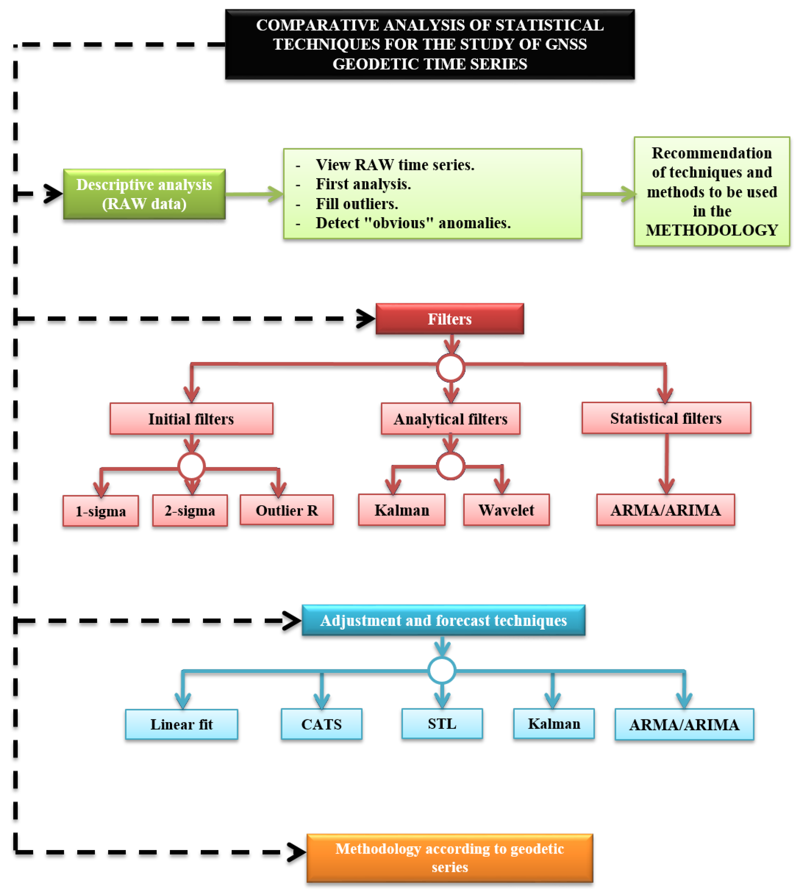
To eliminate or reduce the noise level of the series, various time series filtering techniques were considered, methodologically grouped into initial filters (1–$\sigma$, 2–$\sigma$, Outlier R), analytical filters (Kalman, wavelets), and statistical filters (ARMA/ARIMA). Once this process was carried out, adjustment techniques were applied in order to extract the information on the geodynamic behavior of the GNSS series considered. In this process, it was essential to clearly define the objective pursued and the series to be analyzed. A distinction was made between the horizontal components (east, north) and, on the other hand, the vertical component (elevation) between linear and non-linear behaviors, between series that present anomalies due to events of a tectonic or volcanic nature, etc. All this made it impossible to establish a single procedure for each and every one of the GNSS geodetic series. Rather an adaptation of techniques and methods was carried out according to the geodynamic process under study. Figure 1 shows the adjustment techniques used in this work: linear adjustment, Create and Analyze Time Series (CATS), Seasonal-Trend Loess Decomposition (STL), Kalman Adjustment, and ARMA/ARIMA. These procedures developed were all carried out in R software.

These procedures are succinct and conceptually described below, resulting, however, in a greater depth in those that, due to their specificity, are practically exclusive for the GNSS series.

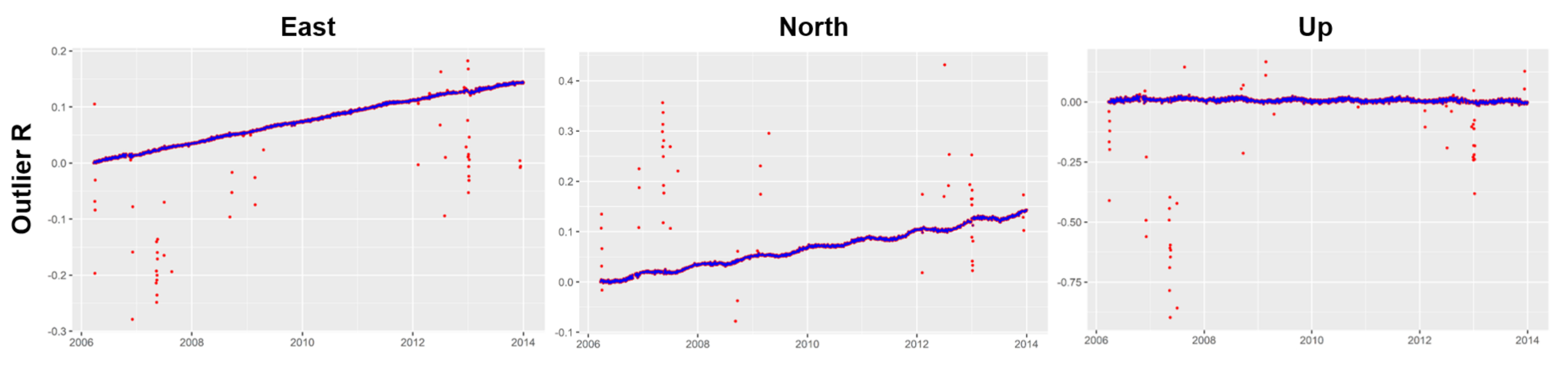
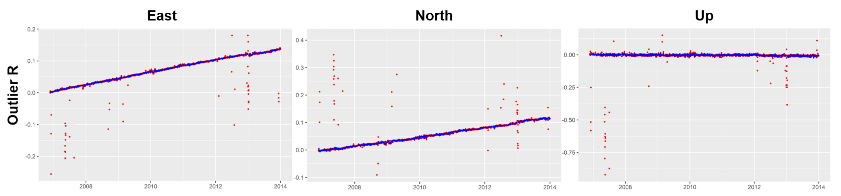
3.1. Initial Filters of the Series

The objective of any initial filtering, which was applied to the GNSS series, consists of the elimination of data with very different values, outliers, from the rest of the series. The 1$\sigma$ and 2$\sigma$ filters are based on the distance of the series points from a simple linear regression line. Depending on the chosen filtering, a greater (1$\sigma$) or less (2$\sigma$) number of data is eliminated from the series. In the case of non-linear series, this process is carried out by linear sections within the series. On the other hand, R contains a package, forecast, to filter time series data that are based on the Box–Cox transform [7,8], which is done by the tsoutliers() function. It was used to achieve greater linearity, homoscedasticity, and a tendency to a normal distribution of the values of the series.

3.2. Predictive Filtering: Kalman, ARIMA, ARMA

3.2.1. Kalman

For this filtering, it is necessary to know what the dynamic linear models are like. Assuming they are known, we proceed to define the Kalman filtering. The Kalman filter is of a predictive–corrective type; as the parameter ${\theta }_t$ that determines the state of the model at time t is calculated, and the estimation of the observations of the series is calculated [9]. Assuming ${\theta }_0\sim N(m_0,C_0)$:

$${\theta }_t=G_t{\theta }_{t-1}+c_i+R_i{W}_t$$

To calculate the estimate of the data of the series, the following is used:

$$y_t=F_t{\theta }_t+d_t+v_t$$

3.2.2. ARIMA Model

ARIMA (integrated moving average autoregressive) models are given by the $ARIMA(p,d,q)$, deal with stationary time series, and are made up of three models: the autoregressive (AR), the integrated (I), and the mean mobile (MA) model, which are defined, respectively, by p, d, and q. By uniting these three models, we get the ARIMA model, which is given by:

$${\varphi }_p\left(B\right){(1-B)}^d{Y}_t={\varphi }_0+{\theta }_q\left(B\right)e_t$$

where $e_t$ represents the errors produced at time t and $Y_t$ of the data of the series. Additionally:

$${\varphi }_p\left(B\right)=1-{\varphi }_{1}B-{\varphi }_2{B}^2-\dots -{\varphi }_p{B}^p$$

$${\theta }_q\left(B\right)=1-{\theta }_{1}B-{\theta }_2{B}^2-\dots -{\theta }_q{B}^q$$

where B is the delay operator.

3.2.3. ARMA Model

ARMA models, defined by $ARMA(p,q)$, deal with non-stationary series and are given by the union of autoregressive models (AR (p)) and moving average models (MA (q)). Therefore, by joining the expressions of both models, we obtained the expression of the ARMA model:

$${\varphi }_p\left(B\right)Y_t={\varphi }_0+{\theta }_q\left(B\right)e_t$$

where ${\varphi }_p\left(B\right)$ and ${\theta }_q\left(B\right)$ are defined in the same way as in the ARIMA model.

3.3. Wavelet Analysis

The wavelet transform decomposes a signal using functions (wavelets) well localized in both the physical space (time) and spectral space (frequency), generated from each other by translation and dilation [10]. The wavelet continuous transform tries to express a signal $x\left(t\right)$, continuous in time, by an expansion of proportional coefficients to the inner product between the signal and different scaled and translated versions of a function prototype $\psi$. This function, known as the mother wavelet or wavelet function, provides a decomposition of the data in the time-frequency plane, along with successive scales. This time-frequency transformation depends on two parameters, the scale parameter a, which is related to the frequency, and the time parameter b, related to the translation of function $\psi$ in the time domain. The continuous wavelet transform is obtained by:

$$CWT(a,b)=\frac{1}{\sqrt{a}}{\int }_{-\infty }^{\infty }x\left(t\right)\psi \left({\displaystyle \frac{t-b}{a}}\right)$$

where $\psi$ is the mother wavelet.

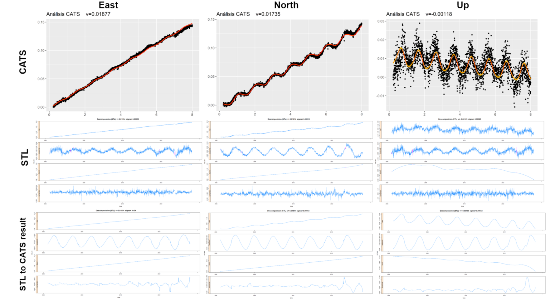
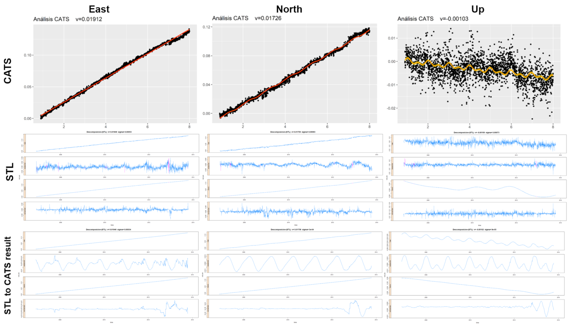
3.4. CATS Analysis

CATS adjustment (Create and Analyze Time Series) is based on stochastic analysis of the GNSS series using Maximum Likelihood Estimation (MLE). This estimate is optimal for the study of noise in a time series. This method makes it possible to simultaneously estimate the noise amplitudes, the linear trend, the periodic signal, and the amplitudes of the existing discontinuities, as well as the uncertainty of these parameters [11]. This setting makes it possible to differentiate between the linear and non-linear parts of the series. The linear part includes the calculation of outliers, the trend, sudden jumps (e.g., earthquakes), and sinusoidal terms. In non-linearity, different types of specific noise models are solved, e.g., white noise and power noise. For the analysis of the GNSS coordinate series, the following functional model is considered:

$${\displaystyle x\left(t\right)=a+bt+\sum _{j=1}^2(Asin\left({\omega }_{j}t\right)+Bcos\left({\omega }_{j}t\right))+\sum _{j=1}^n{C}_{j}H(t-T_j)}$$

where x is the value of the GNSS coordinate at time t; a is the initial value; b is the velocity; ${\omega }_1$ and ${\omega }_2$ are the angular frequencies of the annual and semi-annual harmonic components; and $A_j$ and $B_j$ are the amplitudes of the sine and cosine, respectively. The coefficients $C_j$ are the magnitudes of the discontinuities described by the following Heasivide function:

$${\displaystyle H\left(\tau \right)=\left\{\begin{array}{cc}0& si\tau <0\\ 1& si\tau \ge 0\end{array}\right.}$$

and the time instant of the discontinuity $T_j$. The number of discontinuities in each series is given by n. Therefore, the parameters to be estimated are the initial value a, the velocity b, the sine and cosine amplitudes of the annual and semi-annual harmonic components $A_j$ and $B_j$, and the coefficients $C_j$ of the magnitudes of the discontinuities considered.

To estimate the noise components using the MLE, the probability function is maximized by fitting the covariance matrix of the data. The resulting expression is given by:

$$lik(\widehat{v},C)=\frac{1}{{\left(2\pi \right)}^{\frac{N}{2}}{\left(detC\right)}^{\frac{1}{2}}}{e}^{-0.5{\widehat{v}}^T{C}^{-1}\widehat{v}}$$

Taking the natural logarithm, we obtain:

$$MLE=ln\left[lik(\widehat{v},C)\right]=-\frac{1}{2}[ln\left(detC\right)+{\widehat{v}}^T{C}^{-1}\widehat{v}+Nln\left(2\pi \right)]$$

where N is the number of epochs or observations, C is the covariance matrix of the data, and $\widehat{v}$ are the post-fit residuals of a model applied to the original series using least squares with the same covariance matrix C.

Therefore, we are going to assume that the matrix C is a combination of two sources of error, a white noise component and a power series noise component, so that:

$$C=a_{\omega }^{2}I+b_k^2{J}_k$$

where $a_{\omega }$ and $b_{\omega }$ are the amplitudes of white noise and color noise, respectively. The identity matrix, I, is the covariance matrix of the white noise evoking independence in the time of this type of process. The matrix J_k is the noise covariance matrix of a power series with a spectral index k and is calculated by means of fractional models integrated in such a way that:

$$J_k=T{T}^T$$

where T is a transformation matrix obtained from:

$$T=△T^{-k/4}=\left(\begin{array}{ccccc}{\psi }_0& 0& 0& \cdots & 0\\ {\psi }_1& {\psi }_0& 0& \cdots & 0\\ {\psi }_2& {\psi }_1& {\psi }_0& \cdots & 0\\ ⋮& ⋮& ⋮& \ddots & ⋮\\ {\psi }_{n-1}& {\psi }_{n-2}& {\psi }_{n-3}& \cdots & {\psi }_0\end{array}\right)$$

where $△T$ is the sample interval and,

$${\psi }_n={\displaystyle \frac{{\displaystyle \frac{k}{2}}(1-\frac{k}{2})\dots (n-1-{\displaystyle \frac{k}{2}})}{n!}}={\displaystyle \frac{\mathsf{\Gamma }(n-{\displaystyle \frac{k}{2}})}{n!\mathsf{\Gamma }(-{\displaystyle \frac{k}{2}})}}$$

When n tends to inf, ${\psi }_n$ can be approximated by

$${\psi }_n=\frac{n^{-{\displaystyle \frac{k}{2}}-1}}{\mathsf{\Gamma }(-\frac{k}{2})}$$

Therefore, using MLE, we could fit the coordinate time series to a standard model accurate acoustic by estimating the noise amplitudes for a model, assuming that it is a combination of white noise and power series noise (WN + PLN, is say, White Noise + Power-Law Noise). This approach is based on the recent general formula of the covariance matrix for a power series process, allowing us to estimate noise amplitudes and spectral index together with the rest of the parameters of the station’s motion model.

The stochastic properties and the linear parameters were adjusted together in one way, iterative through a function, to maximize them. The function to be maximized chose a model noise level and estimated the linear parameters, on which a new set of waste was calculated. Using these residuals and the covariance matrix, the value of likelihood and a new noise model with a higher likelihood value were chosen. This process was repeated until the likelihood function reached its maximum value.

3.5. STL Decomposition

STL decomposition (Seasonal and Trend decomposition procedure based on Loess) additively decomposes a time series into its three components trend, seasonality, and irregularities [12]. The time series can contain gaps due to various factors. These do not have a negative influence on the decomposition of the time series. Local regression (Loess) was used to estimate the three components of the series. STL decomposition consisted of two processes: internal and external. In the internal process, in each position, the values of the trend and seasonality components were estimated and updated with the Loess regression. In the external process, the irregularities component of the series was obtained. The trend and seasonality components were smoothed. However, both components were affected by the variation of the series, which could be solved by applying a filter to the seasonality component. This filter was composed of three models of moving averages and the Loess regression [12].

4. Application of Methodology Developed and/or Adapted R

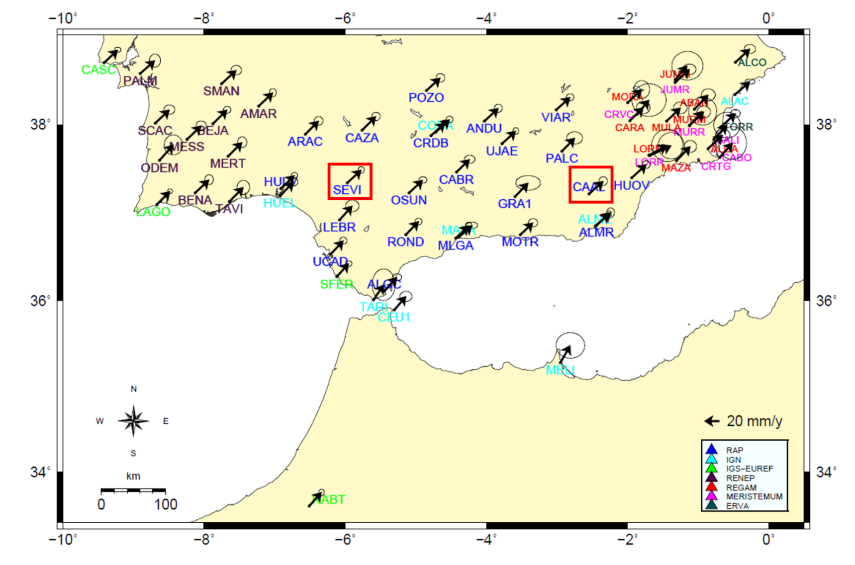
4.1. Description of Selected Series from the Spina Network

Selected time series came from permanent geodetic stations located in the south of the Iberian Peninsula and North Africa, which constitute the SPINA network. This geodetic network is composed of 7 networks of permanent GPS stations: RAP, MERISTEMUM, IGS, IGN, REGAM, RENEP, and ERVA. Each of these networks is made up of GPS stations located in Andalusia, Murcia, the Valencian Community, the south of Portugal, and the north of Africa [10]. We used the position time series derived from daily observations and processed the positioning with respect to the IGS station located in Villafranca (VILL) to get site displacements. Figure 2 shows the horizontal displacement rates at GPS sites in the south of the Iberian Peninsula and North Africa, estimated from GPS time series data (January 2005 to January 2014) [13]. All GPS solutions were realized in the ITRF2005 global reference frame.

4.2. Results

The filters explained in this work were applied to the time series of the SEVI and CAAL stations. Figure 3, Figure 4, Figure 5 and Figure 6 show the results of the SEVI station and, Figure 7, Figure 8, Figure 9 and Figure 10 show the results of the CAAL station.

5. Conclusions

GNSS time series analysis seeks to know the behavior and level of existing geodynamic activity. The geodynamic model is obtained from the velocities of the displacements of each station in the region. That is the starting point for the calculation of the stress and strain models. The GNSS experimental process involves multiple factors that can introduce deviations and dispersions in the values of the GNSS series and, consequently, in the models and results obtained.

In this work, a brief review of analysis techniques and methods for GNSS time series was carried out. Filtering, filtering–fitting, and fitting techniques were analyzed. The need for a descriptive analysis of the RAW series was previously established. Anomalous values, gaps, and dispersion of the series were detected. It was also used to detect changes in the trend or seasonality of the GNSS series.

Among the exclusive filtering techniques, outliers R was more effective and adaptable for both linear and non-linear series, whereas the processes 1$sigma$ and 2 $sigma$, especially in non-linear cases, were not applicable to the entire series.

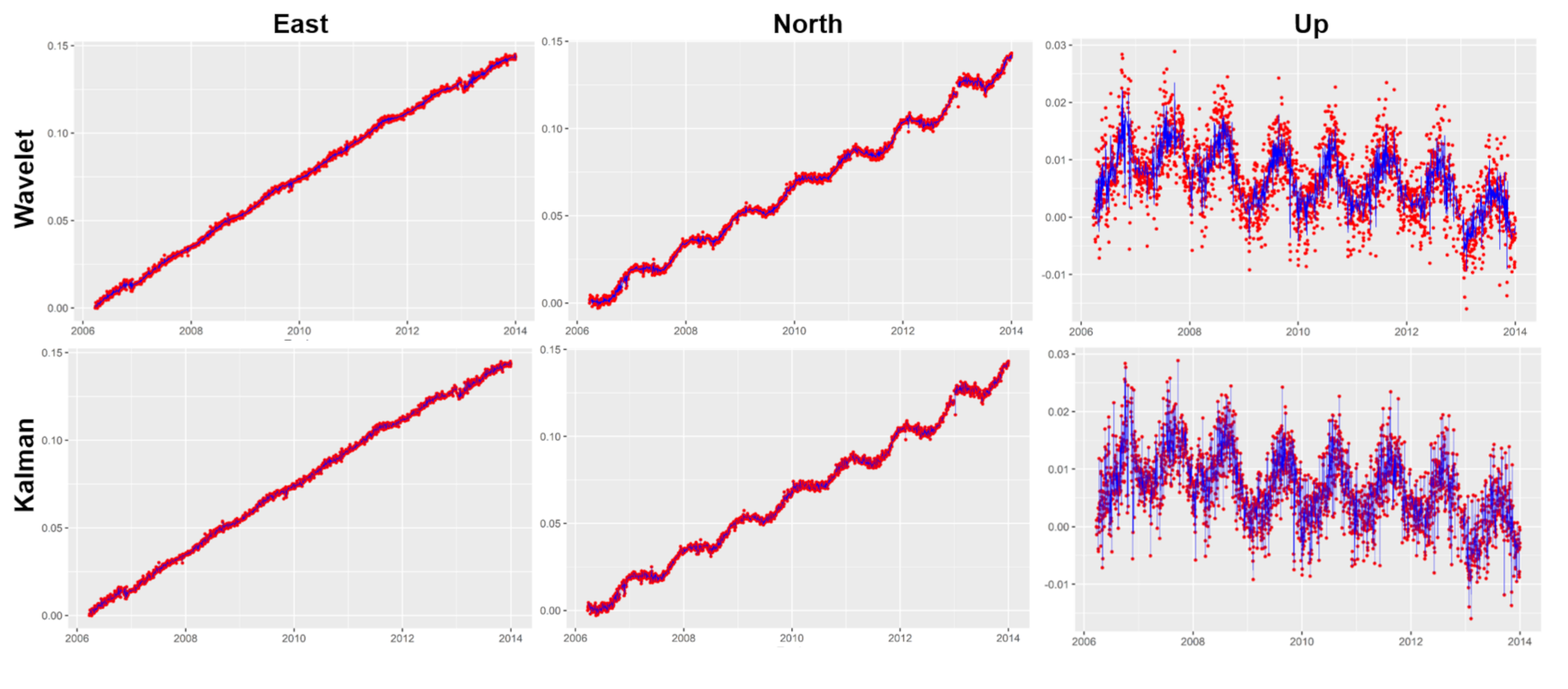
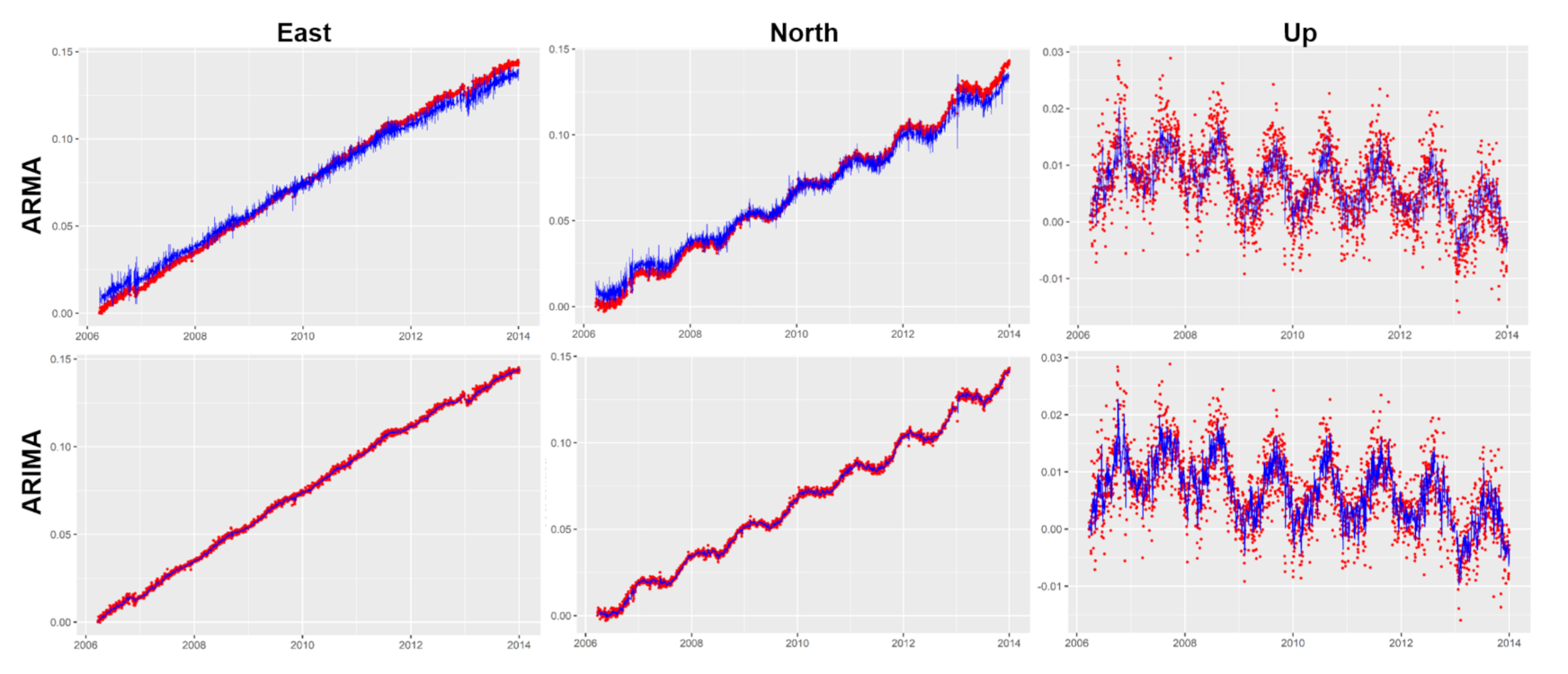
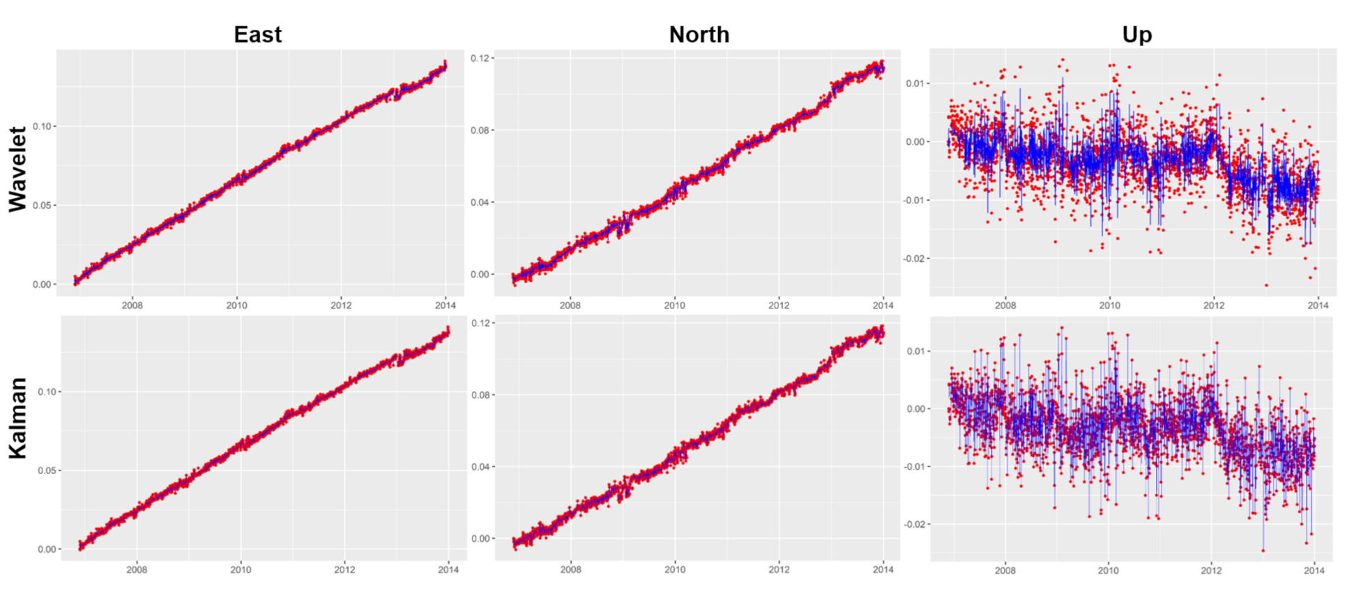
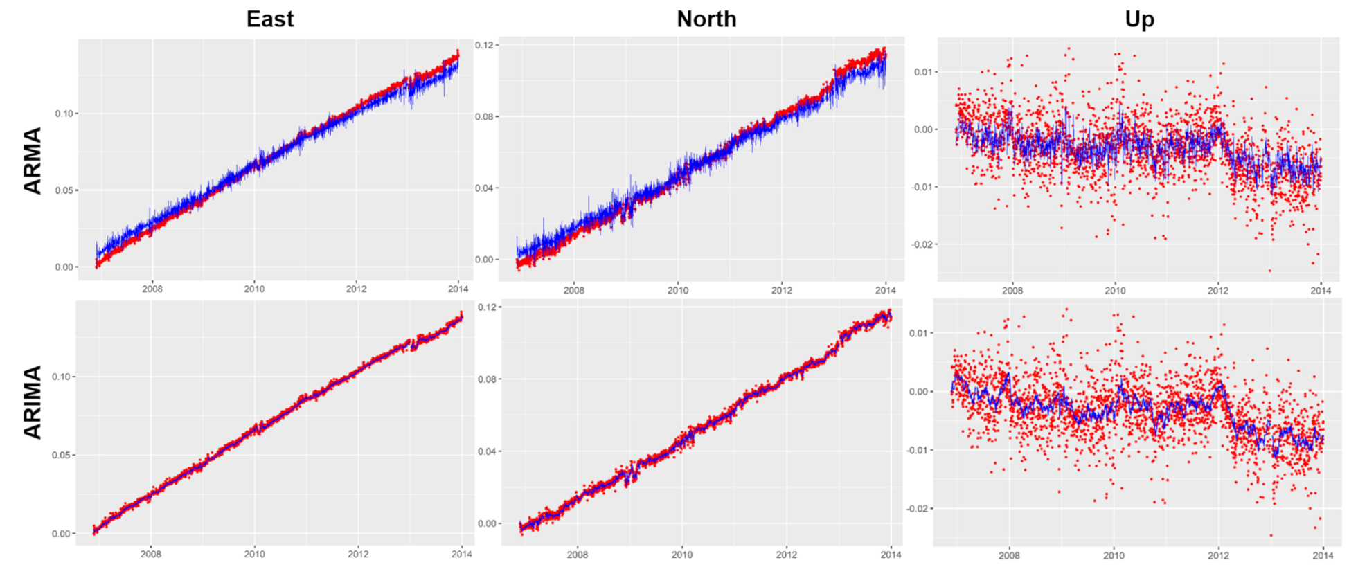
The following were considered as filtering–fitting techniques: Kalman, ARMA/ARIMA, and wavelets. The Kalman and ARMA filters presented more dispersion in the result than ARIMA and wavelets. In series fitting, Kalman and ARIMA obtained smoother curves than ARMA and wavelets, and, therefore, they were more effective in forecasting series. ARIMA and wavelets better adjusted those internal changes in the series providing information on the level of geodynamic activity and the possible detection of seismic events.

CATS-R software provided a series of adjustments, adapted to controlled changes on antenna changes, receivers, firmware, etc. It is a very reliable technique when calculating velocities and, especially, when fitting the elevation component. The STL package that allowed decomposition of the time series into trend, seasonal, and reminder and was analyzed and applied. Its versatility and precision were verified once any of the other techniques had been applied and the series had been purified of adverse effects (outliers, gaps, dispersions, deviations, etc.).

Finally, there is no standardized procedure for any time series. Really, the descriptive analysis informs about the processes to consider in its treatment.