Proceeding Paper

Tourism and Big Data: Forecasting with Hierarchical and Sequential Cluster Analysis †

by
Miguel Ángel Ruiz Reina
Department of Theory and Economic History (Staff of Fundamentals), PhD Program in Economics and Business, University of Malaga, s/n, Plaza del Ejido, 29013 Málaga, Spain
Presented at the 7th International conference on Time Series and Forecasting, Gran Canaria, Spain, 19–21 July 2021.
Eng. Proc. 2021, 5(1), 14; https://doi.org/10.3390/engproc2021005014
Published: 28 June 2021
(This article belongs to the Proceedings of The 7th International Conference on Time Series and Forecasting)

Abstract

:
A new Big Data cluster method was developed to forecast the hotel accommodation market. The simulation and training of time series data are from January 2008 to December 2019 for the Spanish case. Applying the Hierarchical and Sequential Clustering Analysis method represents an improvement in forecasting modelling of the Big Data literature. The model is presented to obtain better explanatory and forecasting capacity than models used by Google data sources. Furthermore, the model allows knowledge of the tourists’ search on the internet profiles before their hotel reservation. With the information obtained, stakeholders can make decisions efficiently. The Matrix U1 Theil was used to establish a dynamic forecasting comparison.

1. Introduction

Big Data is a keyword in digitised markets. Technological development and the incorporation of analysis tools have meant a structural change for organisations, firms and institutions. The interpretation and visualisation of complex data are the core of Data Science [1,2]. Technology companies have the most precious asset in a digitised economic environment: information as a competitive advantage [3].
This new digital economy involves reducing information barriers in markets where intermediaries traditionally existed [4]. Consumers, through their searches on the internet, reveal their intentions. These intentions can be used as a predictive modelling tool for future demands of certain products. Hotel demand in a globalised market can be described through searches for potential consumers [5]. Researchers have paid attention to the selective secondary data sources of the internet network. This means a contribution to traditional analysis [6,7].
Methodologies currently applied have attempted to examine regularities in consumer behaviour data [8,9,10]. The difficulty lies in trying to explain quantitative and qualitative aspects in the modelling. In the field of time series with high dimensions and complex Big Data problems, attention has been paid to concepts such as “The Freedman’s Paradox using an Info-Metrics perspective” [11] or “the power of Text in multidimensional contexts with high frequency” [12].
This article is interested in constructing a Hierarchical and Sequential Cluster Analysis (HSCA) for discrete time series. The analysis carried out focused on the decision-making mechanisms of economic agents for the demand for Hotel Accommodation in Spain (HADS). In particular, there are several generic words that consumers search for on the internet that reveal their intention of HADS. Google Trends (GT) provides an amount of information, which is used in this paper. A better understanding of previous searches can be translated into modelling inputs for structuring the forecasting of HADS.
The contribution of this paper is an improvement to current articles in the literature. The previous methodology has been proven to be an adequate input as a predictive tool, but it lacks classification and hierarchy by topics. The inclusion of a cluster of keywords (124) will allow identifying and segmenting potential consumers. The GT search indexes are for keywords related to tourist interest to visit Spain, and “broad matching” has been used [13,14]. This modelling could be used on internet forecasting for the tourism industry and hospitality, among other fields. Once a volume of temporary searches is known, companies will adjust the offers to their consumers, and there will be a gain in efficiency in decision-making. This fact allows us to model consumer behaviours and to project the regularities of the online tourism market.
Periodicity is essential to reveal systematic behaviours. As we previously cited, a Big Data analysis’s difficulty lies in combining qualitative and quantitative research while maintaining traditional modelling standards. We will build the predictions on discrete-time-series variables and seasonal variable dummies (sampling January 2008 to December 2019).
The HSCA method is compared with SARIMA models [15], ADRL + SEASONALITY model [5], Hierarchical Neural Networks (HNN) [16] and Singular Spectrum Analysis (SSA) [5,8]. As a model selection criterion for forecasting, we will use the Matrix U1 Theil decision matrix [5]. The results obtained from the HSCA methodology reveal improvements in predictive capacity about the other models.
The remainder of this investigation is as follows: Section 1.1 provides a review of the existing literature on the forecasting of Big Data applied to Tourism; in Section 2, the theoretical methodology is performed; in Section 3, data analysis of primary and secondary data sources is done; Section 4 is dedicated to discussing the empirical results obtained after applying the methods proposed. Finally, Section 5 is for the mains conclusions obtained and bibliographic references.

1.1. Literature Review

The grouping in time series occurs when we are interested in the collection into categories or clusters. Nowadays, the application is interesting for finance, economics, medicine, engineering, or computing [17,18,19]. Clustering approaches for time series are time series clustering by features [20,21,22], clustering models in time series [23,24,25], or dependency clustering models [26,27].
Regarding predictive modelling of the use of GT, it should be noted that it is relatively recent. The new datasets from Google resources are a disruptive change in the traditional analysis of HDAS worldwide. The model’s predictive capacity evolution was determined by techniques previously developed by mathematicians and statisticians. The conventional scientific research was joined by technology development, meaning a breakthrough summarised in Big Data Technologies.
In the scientific literature published using GT in tourism, we would highlight studies with an extensive literature review [9,10], or new modelling and forecasting developments. These studies have found standard results in the forecasting techniques concerning other fields such as parametric and non-parametric techniques [8].
In recent years, authors have published papers with secondary databases from Google. In addition, Neural Networks, Machine Learning, Statistical Methods, and traditional Econometrics have been used as forecasting methods in the tourism sector. Recently, attention has been paid to the spurious relationship between GT Searches and tourism demand [14].
Hierarchical algorithm approaches for clusters have been applied to tourism but have always been used to cross-section data. In particular, secondary data obtained from the travel and tourism competitiveness index are analysed to create clusters. Subsequently, multidimensional scaling techniques are applied to detect the most and most minor influential determinants in tourist destinations’ competitiveness [28].
Moreover, a causality method called Granger Causality and seasonality testing has recently been developed, supposing an improvement to Granger’s traditional process of causality [5,29,30]. Furthermore, a new dimensionless model selection criterion has recently emerged called the Matrix U1 Theil. This new criterion is a comparative advantage compared to usual forecasting criteria such as Root of the Mean Square Error, Mean Absolute Error, Theil inequality index, and Diebold–Mariano criterion [5].

2. Methods

This methodological section will develop a new cluster criterion named Hierarchical and Sequential Clustering Analysis (HSCA). This grouping methodology was designed to classify the amount of information existing on the internet network. HSCA will improve and overcome the limitations of keywords previously used in econometric modelling [5]. For this, some properties are cited for modelling with large volumes of data. The first property is Effectiveness and Replicability criteria; the use of HSCA can be replicated in other fields related to Big Data. A second property, identifying clusters with correlation and testing criteria, reveals the importance and causality in our explanatory variables’ modelling. A third property, Noise Tolerance and Outliers Values working with large volumes of data, makes the usual theoretical assumptions to be relaxed in favour of accessible interpretation and usability of the model. Finally, a property, Parsimony Criterion, will determine the best model with the least number of explanatory variables.
In real Big Data applications, it is not easy to find a single algorithm that meets the properties described above. The diagram (Figure 1) represents the sequence from a universe of words related to a variable of interest to predict. The graph shows how the keywords initially relate to each cluster and the predicted variable.

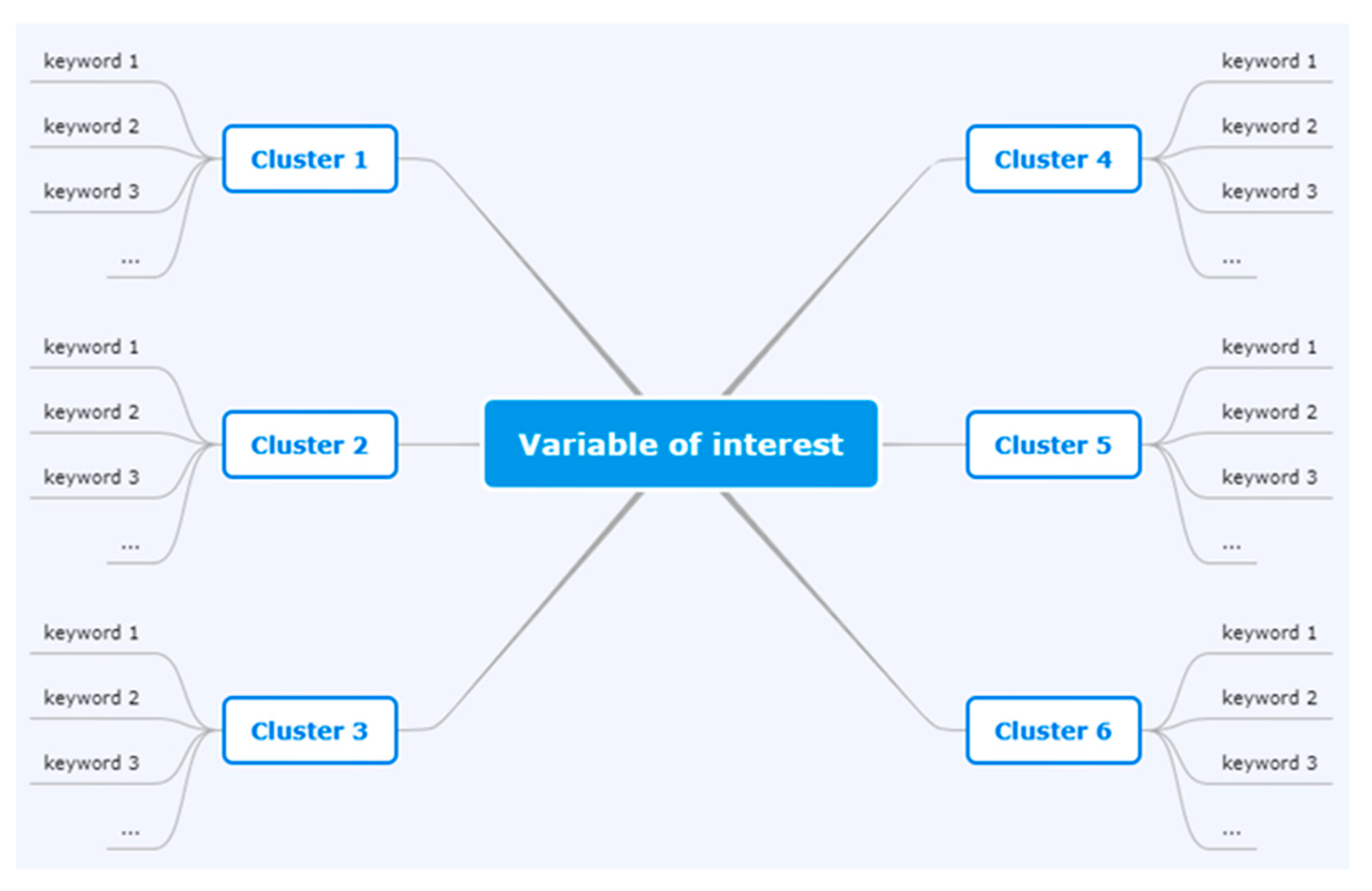
2.1. Hierarchical and Sequential Clustering Analysis (HSCA)

In this subsection, we will describe the HSCA method. We could divide the methodology into the following sequential steps:
First step: Relevant explanatory variables ( k e y w o r d s t ) are selected for forecasting { k e y w o r d s m t     + ;   m = 1 , 2 , 3 ;   t     Τ = 1 , 2 , 3 T } .
In our model, k e y w o r d s t are words that future consumers search on the internet before their tourist demand, for instance, Google searches and “broad matching” such as “visit Spain”, “rent a car in Spain”, or “Weather in Spain” among others. The search words and clusters obtained from GT will be presented in the data section.
Second step: the words of the first step are organised by clusters (topics). { k e y w o r d s m l t     c l u s t e r l t ;       ( c l u s t e r 1 t , c l u s t e r 2 t , c l u s t e r l t ) ;   l = 1 , 2 , 3 } .
Third step: auxiliary regressions ( y t and ( k e y w o r d m 1 t , k e y w o r d m 2 t , , k e y w o r d m l t ) are expressed in natural logarithms) are performed for the same forecasting variable ( y t ) classified by the cluster. The hierarchy of each group is determined by its R 2 . The models present the same dependent variable, and the explanatory variables are different in each grouping.
y t = f ( c l u s t e r 1 t ) + i = 1 12 α i w i + u 1 t = m = 1 j β m k e y w o r d m 1 t + i = 1 12 α i w i + u 1 t
y t = f ( c l u s t e r 2 t ) + i = 1 12 λ i w i + u 2 t = m = 1 k δ m k e y w o r d m 2 t + i = 1 12 λ i w i + u 2 t
y t = f ( c l u s t e r l t ) + i = 1 12 τ i w i + u 1 t = m = 1 o ψ m k e y w o r d m l t + i = 1 12 τ i w i + u l t
where w i ( f o r   m o n t h l y   d a t a   i = 1 ,   2 , ,   12 ) is a deterministic seasonal dummy and uses the HAC covariance method [31].
w 1 = 1 ,   f o r   o t h e r s   w i = 0 w 1 = 1 ,   w 2 = 1   f o r   o t h e r s   w i = 0 ;   w 1 = 1 ,   w 3 = 1   f o r   o t h e r s   w i = 0 ;   w 1 = 1 ,   w 12 = 1   f o r   o t h e r s   w i = 0
Once the regressions and tests of individual significance of the parameters were made, we determine the most relevant keywords within each cluster. The model selection criteria that verify the clustering procedure developed in this article are the usual ones from Akaike (AIC) and Hannan–Quinn [32]. For instance, to contrast any keyword, we define the null hypothesis as the statement that narrows the model and the alternative hypothesis as the broader one [32].
y t = f ( c l u s t e r 1 t ) + i = 1 12 α i w i + u 1 t = m = 1 j β m k e y w o r d m 1 t + i = 1 12 α i w i + u 1 t H o : β m = 0 H 1 : β m 0
Fourth step: after the most relevant words of each cluster were selected, a final preliminary auxiliary regression is performed with the most pertinent explanatory variables of each group.
y t = f ( c l u s t e r 1 t ) + f ( c l u s t e r 2 t ) + + f ( c l u s t e r l t ) + i = 1 12 ϑ i w i + ε t = = m = 1 j γ 1 k e y w o r d m 1 t + m = 1 k ϕ 1 k e y w o r d m 2 t + + m = 1 l ω 1 k e y w o r d m l t + i = 1 12 ϑ i w i + ε t
The model is simplified under the parsimony criterion, seeking the fewest number of significant explanatory variables with explanatory capacity.
y t = f ( c l u s t e r 1 t ) + f ( c l u s t e r 2 t ) + + f ( c l u s t e r l t ) + i = 1 12 ϑ i w i + ε t = = m = 1 j γ 1 k e y w o r d m 1 t + m = 1 k ϕ 1 k e y w o r d m 2 t + + m = 1 l ω 1 k e y w o r d m l t + i = 1 12 ϑ i w i + ε t
The interpretation of coefficients are elasticities, and the dummy variables are semi-elasticities [33].

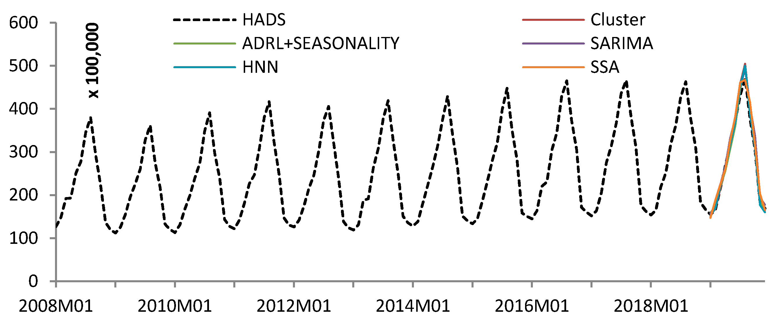
2.2. Comparison of Forecasting and Evaluation
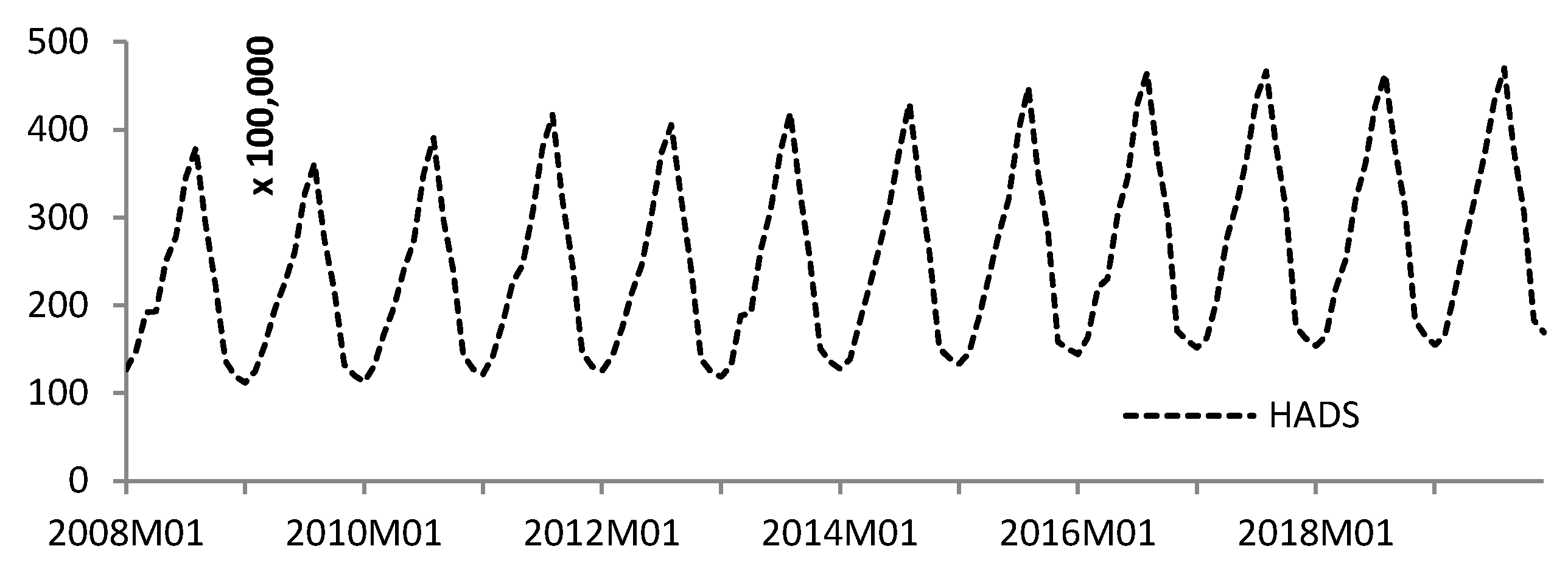
Forecasting and control problems are closely linked. To forecast, we will define the following expression for our modelling as follows:
E ( y t + h | x t , w i ) = E ( m = 1 j γ 1 k e y w o r d m 1 t + h + m = 1 k ϕ 1 k e y w o r d m 2 t + h + + m = 1 l ω 1 k e y w o r d m l t + h + i = 1 12 ϑ i w i )
where h represents the time horizon, and the residuals of the forecasting are white noise { E ( ε t + h | x t + h , w i ) = 0 ;   var ( ε t + h | x t + h , w i ) = σ ε 2 ;   cov ( ε t + h | x t + h , w i ) = 0 } .
As a model selection criterion, we will base ourselves on the Matrix U1 Theil decision matrix. A dimensionless matrix is designed for the decision to select predictive models [5].

3. Data

Data were collected from Jan. 2008 to Dec. 2019. Therefore, we can differentiate two data sources, on the one hand, the official data sources from the INE (Spanish National Statistics Institute (Instituto Nacional de Estadística) https://ine.es/ (accessed on 24 June 2021).) for the predicted variable (HDAS), and the explanatory variables are obtained from Big Data secondary sources, in particular, from the GT tool.
HDAS presents some relevant characteristics in the time series analysis; it is worth noting the high seasonality and a growing trend throughout the period analysed (Figure 2).
From a statistical point of view, it should be noted that the maximum values for each year occur in the summer season, the highest value in August 2019 with 46,998,612 hotel overnights in Spain, and the lowest value in January 2009 with 11,203,819. For the 144 observations analysed (Table 1), the existence of unit roots (ADF (p-value) = 0.85) and stationarity variance (KPSS (p-value) = 0.56) should be highlighted [34,35]. The KPSS (stationary variance) results allow us in our modelling to adjust dummy variables for the repetitive behaviours of the series (seasonality).
The sample period includes 18,000 contemporary observations. From INE data, there are 144 for the variable to be predicted (HADS). The search terms related to planning a visit to Spain were collected from GT and are presented in Table A1 (see Appendix A). In this document, we worked with 17,856 observations of search variables contemporary to the HADS variable. The information is summarised in nine clusters with 124 search terms related to hotel tourism demand from January 2008 to December 2019 for tourists worldwide. All the keywords were searched using “broad match” and combination with other terms. e.g., entering “Spain Hotel”, “Spain culture”, and so on [13].

4. Results

In the following section of empirical results, we describe a training period between January 2008 and December 2018, with a testing sample to forecast 12 months in 2019. The applied methodology is previously mentioned in Section 3Table 2 shows the most relevant keywords within each tourist interest cluster. Regarding the hierarchy, we can indicate that all the keywords finally selected in each group are the most descriptive capacity. For example, finding all values between 0.95 and 0.99, highlighting the terms related to the “social” cluster, which shows that these search engines have a high explanatory capacity, highlighting “Airbnb”, “Youtube”, “English”, “Tripadvisor”, “Twiter”. However, the differences between the clusters and their hierarchy are minimal. An aspect to highlight is that the dummy variables described for systematic seasonality were relevant for all models in all the sets.
Once the main information clusters were selected to predict the variable of interest, we carried out final modelling for the set of variables in the groups to choose the best regressors to evaluate their predictive capacity. In our modelling, we expressed all the variables in natural logarithms, except the seasonal dummy variables, with the p-values in parentheses. We obtain the following result as follows:
y t = 15.90 ( 0.00 ) + 0.08 ( 0.04 ) A i r b n b t + 0.06 ( 0.00 ) A p p l e t 0.12 ( 0.00 ) c a r t + 0.03 ( 0.00 ) c i t y _ b r e a k s t + 0.07 ( 0.00 ) f l i g h t t 0.08 ( 0.00 ) S a m s u n g t + 0.03 ( 0.01 ) s p o r t t + 0.13 ( 0.00 ) v i s a t + 0.07 ( 0.06 ) v i s i t _ S p a i n t + i = 1 12 ϑ i w i
i = 1 12 ϑ i w i = 0.10 ( 0.00 ) w 2 + 0.34 ( 0.00 ) w 3 + 0.50 ( 0.00 ) w 4 + 0.69 ( 0.00 ) w 5 + 0.82 ( 0.00 ) w 6 + 1.05 ( 0.00 ) w 7 + 1.16 ( 0.00 ) w 8 + 0.90 ( 0.00 ) w 9 + 0.69 ( 0.00 ) w 10 + 0.18 ( 0.00 ) w 11 + 0.10 ( 0.00 ) w 12
T = 132 ;   S a m p l e :   2008 M 01   2018 M 12 ;   M e t h o d :   L e a s t   S q u a r e s   H A C   s t a n d a r d   e r r o r s   &   cov a r i a n c e   ( B a r t l e t t   k e r n e l ,   N e w e y - W e s t   f i x e d = 5.0000 ) ; R 2 = 0.99 ;   A d j u s t e d   R 2 = 0.99 ;   A I C = 3.04 ;   P - V a l u e   ( W a l d   F - S t a t i s t i c ) = 0
The final model selected presents a high explanatory capacity R 2 = 0.99 . All the parameter interpretations are studied as the percentage increases of the regressors (1%). For instance, the variable “Airbnb” implies an increase of HADS of 8%; in the explanatory variables, the variables “flight” and “visit Spain” are interpreted as a 7% increase in HADS. It is interesting to mention that the variables “Car” (−0.12) have a negative sign and “flight” (0.07) represents a positive sign. The technological variables (Samsung, Apple), “sports”, and “City Breaks” are relevant.
The prediction of the final HSCA model is compared to other models cited in the Introduction section. The comparative graph of the forecasting time series can be seen in Figure 3.
Table 3 below shows the comparison between the HSCA model and the other predictive models (ADRL + SEASONALITY, SARIMA, HNN, SSA) using Matrix U1 Theil (values more significant than one will indicate better predictive capacity than HSCA; otherwise, we find values less than 1). The HSCA model shows the best predictive power in test h = 3 and h = 6. For a time horizon of h = 12, it would be below ADRL + SEASONALITY and HNN.

5. Conclusions

In the present investigation, a grouping model was developed for hotel accommodation forecasting (HADS). The properties described in the methodological section were central to the research (Section 3). Databases from primary (INE) and secondary (GT) sources were studied. The HSCA model shows a forecasting and causality capacity. A total of 124 Keywords were analysed in a time series from January 2008 to December 2019 (18,000 observations, including HADS). We determined the primary search keywords by topic (Table 2). The hierarchy of each cluster was also fixed.
Furthermore, this research was compared with other models with high predictive capacity, such as ADRL + SEASONALITY: SARIMA, HNN and SSA. Analysing the Matrix U1 Theil results for time horizons h = 3 , we found HSCA (coefficients less than 1) as the best model. For an annual time horizon, we discovered that ADRL + SEASONALITY (1.14) and HNN (1.13) performed better results than HSCA. Let us compare the causal explanatory capacity ( R 2 = 0.99 ). We can say that HSCA is the best since it includes many more explanatory variables (search topics) than the rest of the models studied. With the information obtained from the HSCA model, it is possible to adjust tourist profiles based on their searches. Primary and secondary tourism industries can benefit from this knowledge of the global market.
We can deduce that previous studies’ explanatory capacity was improved from this work, providing relevant and novel information to the scientific literature. Furthermore, this research is the basis for future empirical work related to stakeholders’ Big Data field and decision-making. Currently, the most developed economies are focused on a digital environment. Both firms and consumers are expanding their activities on digital platforms, which makes it possible to measure market actions. Furthermore, the engineering of search engines such as Google comes from valuable information to improve the predictive capacity of the models. The results presented in this study refer to consumers’ active search, but the data generated can generate predictive information for future tourism consumers. The impact on this type of study’s economy supposes a paradigm shift in traditional tourism analysis studies.
The study was applied to the tourism field. However, this methodology can be applied to the finance, insurance or airline field, where decision-making is critical in competitive markets.

Funding

This research received no external funding.

Institutional Review Board Statement

Not applicable.

Informed Consent Statement

Not applicable.

Data Availability Statement

The datasets generated during and analysed during the current study are available in the repository (https://drive.google.com/file/d/1T5_dQGxCLlG7IKMOPvgFUD9lsCe344fn/view?usp=sharing) (accessed on 23 June 2021).

Acknowledgments

The author wishes to acknowledge the support given by the University of Malaga. PhD. Program in Economics and Business, effective from 16 July 2013. Especially to Associate Professor Antonio Caparrós Ruiz from the University of Malaga for reviewing this work. Group of research: “SEJ157-INIDICADORES SOCIALES”.

Conflicts of Interest

The authors declare no conflict of interest.

Appendix A

Table A1. Keywords and clusters correlated with HADS (broad matching). January 2008 to December 2019. Own Elaboration.
SportsLawsTransportSeasonalitySocialWelfareSearchesCulturePlaces
Sport TaxesTransport Weather Spanish PeopleHospitality Trip SpainMonuments Beach
Football Tax freeFlight Winter Mind Environment Visit SpainMusueums Mountain
Basketball LawsTrain Summer vegan SpainRelax Spain TourismCongress Island
Athletics SpainSchengen RoadsAutumn English Stress Hotel SpainStudy nature
Swimming SpainSpain passportCruise ships Spring French Life style Apartment SpainDisco Mediterranean area
Volleyball SpainVisa SpainHelicopter SpainClimate Change Italian Hospital Best travel Concert Canary Island
Tennis SpainSpain travel insuranceBus SpainEaster week SpainGerman Apple SpainResort Food Zoo Spain
Boxing SpainMedical certificate SpainCar SpainChristmas SpainFacebook Android SpainEcotourism Wine Andalusia Spain
Soccer SpainSpain driving licenseTolls Spain-Twitter Samsung SpainFamily Trip theme parks SpainCatalonia Spain
Hockey on ice Spain-Motorhomes Spain-Tripadvisor Xiaomi Spainlow cost nightlife SpainAlcázar de Toledo
Baseball Spain- -Hotels.com SpainHuawei SpainRural SpainSpain architectureMonasterio del Escorial
----Booking.com Spain-Agriculture Spainalcohol Palacio Real
----Wimdu-Fishing SpainCity Breaks Muralla de Ávila
----Kayak Spain-Livestock Spain-Alcázar de Segovia
----Airbnb-Blitz -Valencian Community Spain
----Instagram ---Plaza de España
----Youtube ---Teatro Romano de Mérida
----Terrorism ---Acueducto de Segovia
----Overtourism ---Mezquita de Córdoba
----Tourism Phobia ---Sagrada Familia
----Wifi Spain---La Giralda
----3G, 4G and 5G Spain---La Alhambra and Tours

References

  1. Kleinberg, J.; Lakkaraju, H.; Leskovec, J.; Ludwig, J.; Mullainathan, S. Human decisions and machine predictions. Q. J. Econ. 2018, 133, 237–283. [Google Scholar] [CrossRef]
  2. Carrizosa, E.; Guerrero, V.; Morales, D.R. Visualising data as objects by DC (difference of convex) optimisation. Math. Program. 2018, 169, 119–140. [Google Scholar] [CrossRef] [Green Version]
  3. Mikalef, P.; Pappas, I.O.; Krogstie, J.; Giannakos, M. Big data analytics capabilities: A systematic literature review and research agenda. Inf. Syst. e-Bus. Manag. 2018. [Google Scholar] [CrossRef]
  4. Palos-Sanchez, P.R.; Correia, M.B. The collaborative economy based analysis of demand: Study of airbnb case in Spain and Portugal. J. Theor. Appl. Electron. Commer. Res. 2018. [Google Scholar] [CrossRef] [Green Version]
  5. Ruiz-Reina, M.Á. Big Data: Does it really improve Forecasting techniques for Tourism Demand in Spain? In International Conference on Time Series and Forecasting; Godel Impresiones Digitales S.L.: Granada, Spain, 2019; pp. 694–706. [Google Scholar]
  6. Song, H.; Li, G. Tourism demand modelling and forecasting—A review of recent research. Tour. Manag. 2008, 29, 203–220. [Google Scholar] [CrossRef] [Green Version]
  7. Pan, B.; Wu, D.C.; Song, H. Forecasting hotel room demand using search engine data. J. Hosp. Tour. Technol. 2012, 3, 196–210. [Google Scholar] [CrossRef] [Green Version]
  8. Wu, D.C.; Song, H.; Shen, S. New developments in tourism and hotel demand modeling and forecasting. Int. J. Contemp. Hosp. Manag. 2017, 29, 507–529. [Google Scholar] [CrossRef]
  9. Mariani, M.; Baggio, R.; Fuchs, M.; Höepken, W. Business intelligence and big data in hospitality and tourism: A systematic literature review. Int. J. Contemp. Hosp. Manag. 2018. [Google Scholar] [CrossRef] [Green Version]
  10. Li, J.; Xu, L.; Tang, L.; Wang, S.; Li, L. Big data in tourism research: A literature review. Tour. Manag. 2018, 68, 301–323. [Google Scholar] [CrossRef]
  11. Macedo, P. Freedman’s Paradox: An Info-Metrics Perspective. In International Conference on Time Series and Forecasting; Godel Impresiones Digitales S.L.: Granada, Spain, 2019; pp. 665–676. [Google Scholar]
  12. Gabrielyan, D.; Masso, J.; Uuskula, L. Powers of Text. In International Conference on Time Series and Forecasting; Godel Impresiones Digitales S.L.: Granada, Spain, 2019; pp. 677–693. [Google Scholar]
  13. Choi, H.; Varian, H. Predicting the Present with Google Trends. Econ. Rec. 2012, 88, 2–9. [Google Scholar] [CrossRef]
  14. Bokelmann, B.; Lessmann, S. Spurious patterns in Google Trends data—An analysis of the effects on tourism demand forecasting in Germany. Tour. Manag. 2019, 75, 1–12. [Google Scholar] [CrossRef]
  15. Box, G.E.P.; Jenkins, G.M.; Reinsel, G.C. Time Series Analysis: Forecasting and Control, 4th ed.; John Wiley & Sons: Hoboken, NJ, USA, 2013. [Google Scholar]
  16. Athanasopoulos, G.; Hyndman, R.J.; Kourentzes, N.; Petropoulos, F. Forecasting with temporal hierarchies. Eur. J. Oper. Res. 2017, 262, 60–74. [Google Scholar] [CrossRef] [Green Version]
  17. Liao, T.W. Clustering of time series data—A survey. Pattern Recognit. 2005, 38, 1857–1874. [Google Scholar] [CrossRef]
  18. Aghabozorgi, S.; Shirkhorshidi, A.S.; Wah, T.Y. Time-series clustering—A decade review. Inf. Syst. 2015, 53, 16–38. [Google Scholar] [CrossRef]
  19. Caiado, J.; Maharaj, E.A.; D’Urso, P. Time-series clustering. In Handbook of Cluster Analysis; Chapman & Hall/CRC: Boca Raton, FL, USA, 2015; pp. 241–264. [Google Scholar]
  20. Kakizawa, Y.; Shumway, R.H.; Taniguchi, M. Discrimination and clustering for multivariate time series. J. Am. Stat. Assoc. 1998, 93, 328–340. [Google Scholar] [CrossRef]
  21. Scotto, M.G.; Alonso, A.M.; Barbosa, S.M. Clustering time series of sea levels: Extreme value approach. J. Waterw. Port Coast. Ocean Eng. 2010, 136, 215–225. [Google Scholar] [CrossRef]
  22. D’Urso, P.; Maharaj, E.A.; Alonso, A.M. Fuzzy clustering of time series using extremes. Fuzzy Sets Syst. 2017, 318, 56–79. [Google Scholar] [CrossRef]
  23. Alonso, A.M.; Berrendero, J.R.; Hernández, A.; Justel, A. Time series clustering based on forecast densities. Comput. Stat. Data Anal. 2006, 51, 762–766. [Google Scholar] [CrossRef]
  24. Scotto, M.G.; Barbosa, S.M.; Alonso, A.M. Model-based clustering of Baltic sea-level. Appl. Ocean Res. 2009, 31, 4–11. [Google Scholar] [CrossRef]
  25. Vilar, J.A.; Alonso, A.M.; Vilar, J.M. Non-linear time series clustering based on non-parametric forecast densities. Comput. Stat. Data Anal. 2010, 54, 2850–2865. [Google Scholar] [CrossRef]
  26. Alonso, A.M.; Peña, D. Clustering time series by linear dependency. Stat. Comput. 2019, 29, 655–676. [Google Scholar] [CrossRef]
  27. Alonso, A.M.; Galeano, P.; Peña, D. A robust procedure to build dynamic factor models with cluster structure. J. Econom. 2020, 216, 3552. [Google Scholar] [CrossRef]
  28. Chávez, J.C.N.; Torres, A.I.Z.; Torres, M.C. Hierarchical Cluster Analysis of Tourism for Mexico and the Asia-Pacific Economic Cooperation (APEC) Countries. Rev. Tur. Anál. 2016, 27, 235–255. [Google Scholar] [CrossRef] [Green Version]
  29. Granger, C.W.J. Investigating Causal Relations by Econometric Models and Cross-spectral Methods. Econometrica 1969, 37, 424–438. [Google Scholar] [CrossRef]
  30. Ruiz-Reina, M.Á. Forecasting using Big Data: The case of Spanish Tourism Demand. In International Conference on Time Series and Forecasting; Godel Impresiones Digitales S.L.: Granada, Spain, 2019; pp. 782–789. [Google Scholar]
  31. Newey, W.K.; West, K.D. A Simple, Positive Semi-Definite, Heteroskedasticity and Autocorrelation Consistent Covariance Matrix. Econometrica 1987, 55, 703–708. [Google Scholar] [CrossRef]
  32. Greene, W.W.H. Econometric Analysis, 7th ed.; Prentice Hall: Hoboken, NJ, USA, 2012. [Google Scholar]
  33. Peng, B.; Song, H.; Crouch, G.I.; Witt, S.F. A Meta-Analysis of International Tourism Demand Elasticities. J. Travel Res. 2015, 54, 611–633. [Google Scholar] [CrossRef]
  34. Dickey, D.A.; Fuller, W.A. Likelihood Ratio Statistics for Autoregressive Time Series with a Unit Root. Econometrica 1981, 49, 1067–1072. [Google Scholar] [CrossRef]
  35. Kwiatkowski, D.; Phillips, P.C.B.; Schmidt, P.; Shin, Y. Testing the null hypothesis of stationarity against the alternative of a unit root. How sure are we that economic time series have a unit root? J. Econom. 1992, 54, 159–178. [Google Scholar] [CrossRef]
Figure 1. Clustering scheme for a predictive variable (Variable of interest). Own Elaboration.
Engproc 05 00014 g001
Figure 2. Number of HADS (January 2008 to December 2019). Data source: INE. Own Elaboration.
Engproc 05 00014 g002
Figure 3. Out-sample forecast HADS h = 12 (January 2018 to December 2019). Own Elaboration.
Engproc 05 00014 g003
Table 1. Descriptive Statistics and Stationary Analysis of HADS (Jan. 2008 to Dec. 2019). Own Elaboration.
MeanMaximumMinimumADF (p-Value)KPSS (p-Value)Observations
24,989,87446,998,61211,203,8190.850.56144
Table 2. Summary of clusters and keywords (broad matching) relevant for HADS. Sample January 2008–December 2018. Own Elaboration.
ClusterRelevant KeywordsR-Squared
Sportssport0.95
Lawsvisa0.97
Transportcar, flight0.98
Seasonalitysummer, winter0.95
SocialAirbnb, Youtube, English, Tripadvisor, Twiter0.99
WelfareAndroid, Xiaomi0.98
Searcheslow-cost, Spain Tourism, visit Spain0.98
Culturealcohol, city breaks, monuments, architecture0.97
PlacesBeach, Canary Island, Alhambra, Plaza de España, Sagrada Familia0.98
Table 3. Summary of forecasting accuracy. Out-Sample training Jan. 2019–Dec. 2019. Own Elaboration.
HSCAADRL + SEASONALITYSARIMAHNNSSA
HSCA (h = 3)1.000.390.360.430.15
HSCA (h = 6)1.000.500.690.920.39
HSCA (h = 12)1.001.140.861.130.79
Publisher’s Note: MDPI stays neutral with regard to jurisdictional claims in published maps and institutional affiliations.

