Abstract
A computationally efficient predictive digital twin (DT) of a small-scale greenhouse needs an accurate and faster modelling of key variables such as the temperature field and flow field within the greenhouse. This involves: (a) optimally placing sensors in the experimental set-up and (b) developing fast predictive models. In this work, for a greenhouse set-up, the former requirement fulfilled first by identifying the optimal sensor locations for temperature measurements using the QR column pivoting on a tailored basis. Here, the tailored basis is the low-dimensional representation of hi-fidelity computational fluid dynamics (CFD) flow data, and these tailored basis are obtained using proper orthogonal decomposition (POD). To validate the method, the full temperature field inside the greenhouse is then reconstructed for an unseen parameter (inflow condition) using the temperature values from a few synthetic sensor locations in the CFD model. To reconstruct the flow-fields using a faster predictive model than the hi-fidelity CFD model, a long-short term memory (LSTM) method based on a reduced-order model (ROM) is used. The LSTM learns the temporal dynamics of coefficients associated with the POD-generated velocity basis modes. The LSTM-POD ROM model is used to predict the temporal evolution of velocity fields for our DT case, and the predictions are qualitatively similar to those obtained from hi-fidelity numerical models. Thus, the two data-driven tools have shown potential in enabling the forecasting and monitoring of key variables in a digital twin of a greenhouse. In future work, there is scope for improvements in the reconstruction accuracy by involving deep-learning-based corrective source term approaches.
1. Introduction
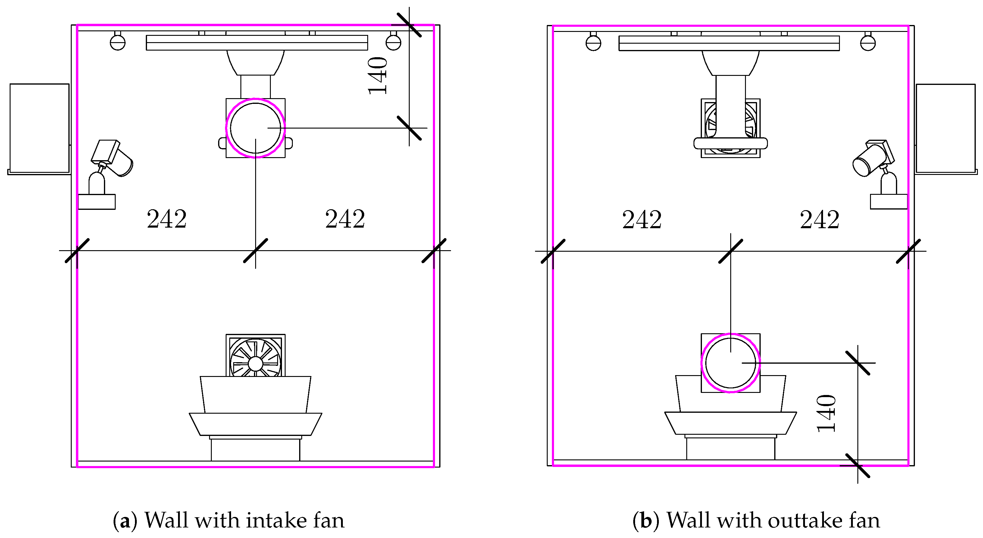
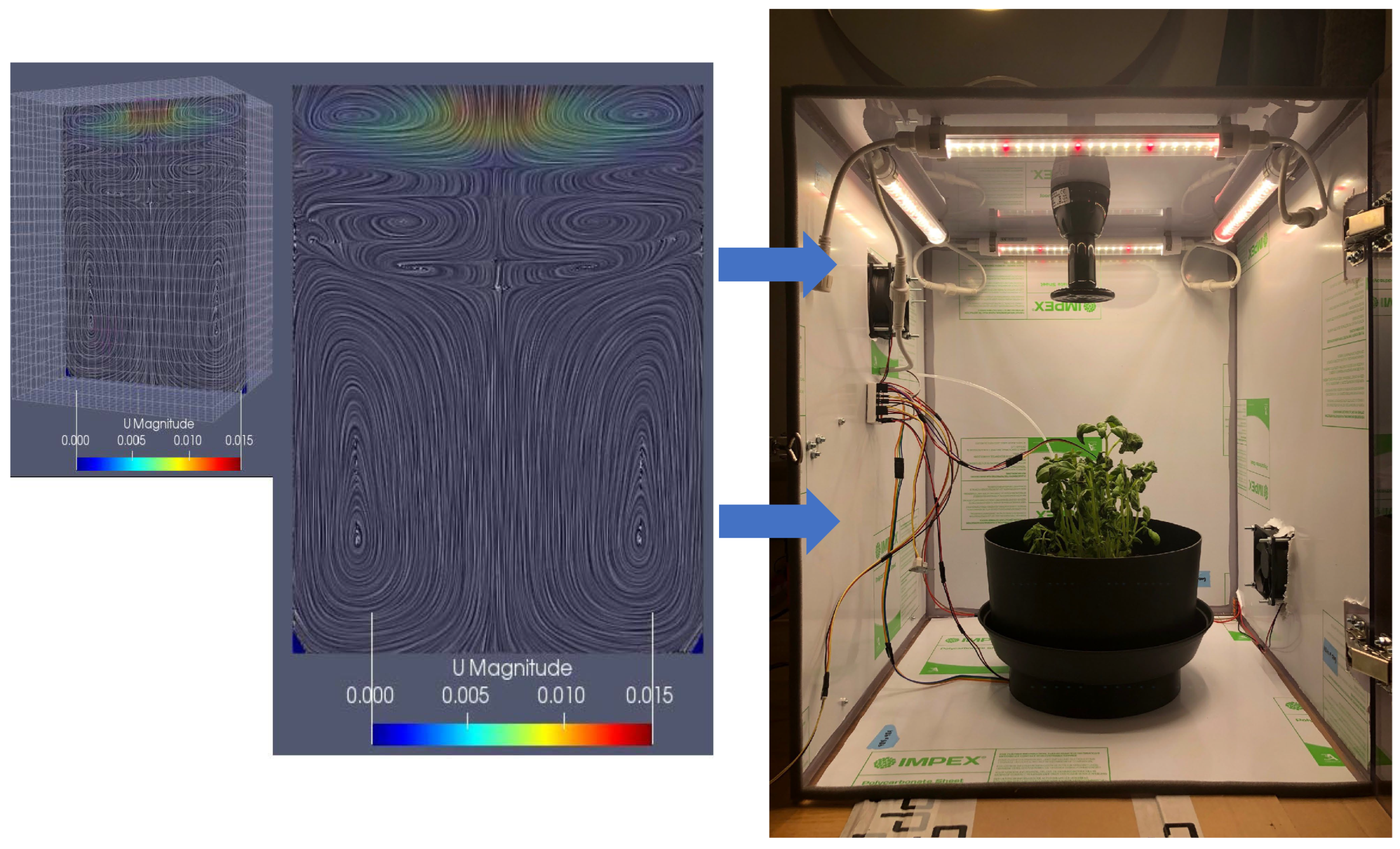
A digital twin (DT) [1] is defined as a virtual representation of a physical asset enabled through data and simulators for real-time predictions, optimization, monitoring, controlling, and improved decision-making. For efficient real-time predictive digital twins, the use of computationally intensive hi-fidelity numerical solvers and a large number of sensors (for control) needs to be avoided, as well as time-series prediction techniques and sparse sensor placement locations. In this work, an experimental greenhouse set-up is constructed (as seen in Figure 1) as the physical asset of DT. The physical asset (Figure 2) has sensors to measure the varying internal conditions (temperature, flow rate, humidity) inside a fully controllable environment, but requires optimal sensor placements to enable the reconstruction of a full field using only the measured sensor values.
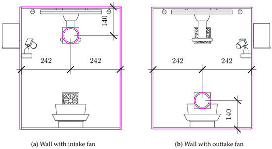
Figure 1.
Schematic showing the layout of the greenhouse side walls with dimensions in millimeters.
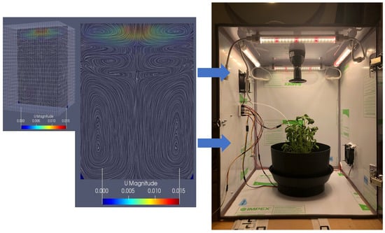
Figure 2.
Bidirectionally coupled DT and Asset.
Determining sensor placements for large data-sets involves methods such as a compressed sensing algorithm [2], which assumes that the original signal is sparse on a universal basis. It then uses the L1-norm-based optimization approach to find the sparsest solution. Once the sparse signal is recovered using compressed sensing (CS), the sensor locations can be identified by examining the non-zero entries in the solution vector. This method does not require training data to find the basis functions as it uses a universal basis. However, this approach is not suitable for high-dimensional physical systems with a known structure, and for such systems, a method based on the data-driven QR pivoting of tailored basis [3] is more suitable. This data-driven approach uses training data to find the basis specific to the known system and this results in a lower number of optimum sensor placements for a high-dimensional system than that obtained using the CS-based method. Hence, the QR-pivoting-based sensor placement method is demonstrated to have applications in a greenhouse digital twin. For DT, there is also a need to develop faster data-driven reduced-order models [4,5,6]) for predicting the temporal flow state of the physical asset. In this work, we employ data-driven techniques involving long-short term memory, proper orthogonal-decomposition-based decomposition and QR-pivoting to enable modelling of the temporal dynamics of key variables for a digital twin of a small-scale greenhouse. The methodology and results are discussed in the next sections, followed by the conclusion.
2. Methodology
The greenhouse set-up (physical set-up) and its hi-fidelity computational fluid dynamics (CFD) set-up are constructed first (Figure 1 and Figure 2). The training data-set of temperature and velocity fields obtained from CFD simulations of the greenhouse set-up (as described in Section 2.1) are then subjected to proper orthogonal decomposition (POD). The POD decomposes the data into the dominant basis functions (which serve as a low-dimensional representation) and accompanying time-dependent coefficients (as discussed in Section 2.2). These dominant basis modes are then used to obtain optimal sparse locations for temperature measurements and to develop a reduced-order model for the flow field. The details of the data-set and methodology are provided below.
2.1. Training Data-Set and Greenhouse CFD Simulations
The training data (i.e., the full temperature field and velocity field across the green-house) needed by the data-driven techniques are generated using a hi-fidelity computational fluid dynamics (CFD) simulation of the greenhouse set-up. Figure 2 shows the experimental set-up and CFD simulation of the greenhouse to enable a digital twin (DT). In this work, a hi-fidelity OpenFOAM CFD solver is used for the simulation, and this solves the Navier stokes equation (i.e., the continuity and momentum conservation equations) along with the thermal equation, while the turbulence is modelled using an RANS k-epsilon model. The greenhouse has a fan to control inlet airflow speed, and a heater on the top of roof for temperature control. These are considered boundary conditions for the CFD solver. For CFD simulations, the parameters that are changed are: (a) Inlet air flow speed due to the fan operation in the greenhouse. For each simulation case, this is varied as follows: 0 m/s (i.e., no in-flow and the natural convective flow occurs due tothe heat flux from the heater at the top), 1 m/s, 2 m/s and 3 m/s; (b) The heat flux at the top is varied to match the expected heater output from the top. The generated simulation data-set is divided into training and validation data-sets to develop and test the data-driven techniques, while the training data-set comprises simulation cases with 0 m/s, 1 m/s and 3 m/s inlet flow conditions. The simulation case of 2 m/s is used to validate/test data-driven reconstructions. The fan speed and heat flux are varied in the real-experimental set-up to enable an optimal temperature for plant growth in the greenhouse. The grid size used for numerical CFD simulation was selected after a proper grid-independence test and the total number of grids was = 14,165. The discretization schemes employed are as follows: linearUpwind for convection term and implicit second-order backward scheme for temporal discretization. The time-step for simulation is selected to ensure the courant number is less than 1 and total time of simulations in each simulation could develop the flow. The snapshots of temperature and velocity from each of the simulation cases are saved at a time-step of about 0.5 s. These snapshots are then subjected to proper orthogonal decomposition (POD) to obtain the dominant basis functions (which serve as a low-dimensional representation) and accompanying time-dependent coefficients (as discussed in Section 2.2). The dominant basis functions are then used to obtain optimal sparse locations for temperature measurements and develop a reduced-order model. The methodology of the LSTM-POD reduced-order model is covered briefly in Section 3.2, and in more detail in [6]. The next section describes the POD methodology and sensor placement methodology.
2.2. Proper Orthogonal Decomposition
The chosen snapshots of the temperature simulations from the training database (i.e., simulations with an inflow of 0 m/s, 1 m/s and 3 m/s, respectively) were flattened in their spacial dimensions to form a matrix , where . The matrix was then shifted by the mean of its columns () and scaled by the standard deviation of its columns () to obtain matrix .
The matrix was decomposed as shown in Equation (2) by using singular value decomposition to obtain the dominant basis functions (i.e the POD modes),
where and are orthonormal matrices, while is only non-zero on its diagonal. The values in the diagonal of are called the singular values of and are ordered in descending order. The columns of are called the POD modes of . By truncating the matrices , and to only use the first r singular values, it can be used for dimensionality reductions. The truncated POD modes serves as low-dimensional representation of hi-dimensional data. The columns of and singular values are ordered by how important they are for the reconstruction of . The truncated singular value decomposition is shown in Equation (3). and are the first r columns of and , respectively, and is a diagonal matrix with the first r singular values on the diagonal. Using the first r POD-modes will lead to some error, represented by the matrix . For many matrices consisting of structured data, the error will be small for a relatively limited choice of r if the first r modes captures most of the variance in the data.
Similarly, any column vector of , or any vector similar enough to the columns of , can be approximated as in Equation (4). The vector can be seen as a low-dimensional representation of .
In this study, the number of POD modes and sparse sensors were both chosen to be . The choice of number of POD modes, r, and the number of sensors, p, is important to the performance of the method. Too small an r or p will lead to a poor performance, while too large an r or p will result in a too large model that might be slow or infeasible to use in practice. A too large p will also defeat the purpose of the method using sparse measurements. More details on the choice of are given in Section 2.4.
2.3. Reconstruction from Sparse Measurement
This section explains how to estimate full-field () from a sparse measurement () given a tailored basis and the sensor locations in .
Here, is a sparse measurement of and is calculated as in Equation (5) where is the measurement matrix and v is measurement noise. The measurement is sparse in the sense that it only contains information about relatively few entries in . The number of elements in is denoted as p and is the number of measurements taken of .
The matrix represents the part of that is measured in . It can be structured in different ways. One way is for each row of to consist of a single 1, with all other entries being 0. Then, each element in will be a direct measurement of a single element in . This case is called sparse sensor placement.
The relationship between and in Equations (6) is found by combining (5) and (4). Furthermore, and can be approximated from , as shown in Equation (7). These approximations are good as long as and are sufficiently small.
Thus, to reconstruct full-field , the condition number of (the row-selected basis matrix—a product of the measurement and basis matrices) should be small so that the input errors are not amplified during the inversion in Equation (8). The condition number of can be controlled by the choice of measurement matrix . A suitable sensor placement algorithm is the one that helps to find rows of corresponding to the point sensor location in state space that provides the optimal conditions for the inversion of matrix . This is obtained by QR pivoting (the chosen sensor location method), as detailed in Section 2.4.
2.4. QR Pivoting for Sparse Sensor Placement
The choice of sensor locations in is important to enable optimal conditioning and inversion operation in Equation (8). The QR-decomposition with column pivoting is proposed as a computationally efficient alternative to finding optimal sensor locations [3]. This is carried out using the first p choices of column pivots when calculating the QR decomposition of in the algorithm as the p sensor locations. Using , one can calculate the QR decomposition of instead. Each row of is a row of zeros besides a single element that is set to 1. The resulting p sensor locations (selected pivots) are then used to find the elements in that should be set to 1. The value i-th chosen pivot is the index of the the element on the i-th row of that is set to 1. The first pivot location is chosen by finding the row of the matrix ( or ) with the largest -norm. The index of this row is the first chosen sensor location. The matrix ( or ) is then modified before the next iteration. Each row is subtracted by the projection of the row on the row corresponding to the chosen sensor location. This is repeated until the desired number of sensor locations is chosen. In this form, the algorithm can easily be modified to include constraints on the possible choices of sensor placement. This can be very useful; for example, if some sensor locations are not practical to use. Another case when this is useful is if one wants a maximum or minimum number of sensors inside an area.
Regarding the choice of number of modes r and number of sensors p in this work, explained variance is often used to chose the number of POD modes. This can be a useful tool to find a lower bound for good choices of number of modes r. Here, first two modes captures most of the variance in both the temperature and velocity fields. However, it is wiser to use a larger r because some time steps might not be modeled well by the POD-modes even tough the explained variance is high. This can happen if many time steps are similar and a few time steps are different from the others. The explained variance might be high because the POD modes model the time steps that are similar to each other. The few time steps that are modeled poorly will not necessarily effect the explained variance. This could be the case in this application, where the time steps toward the end of the simulation are very similar because the system moves toward a steady state. However, the early time steps are very different from the steady state and could therefore be modeled poorly, even though the explained variance is high. Therefore, it is wiser to use a higher r.
However, there are some restrictions to the choice of r and number of sensors p: (a) The first restriction on the choice of r and p comes from the number of elements in the POD-modes. If , the matrix is constructed in the sensor placement algorithm. However, if n is large enough, then constructing and using this matrix is infeasible. In this application, = 141,659, which makes it infeasible to choose . Instead, if , then the matrix is used instead, which makes it much easier to work withfor a small choice of r. (b) Another constraint is that one actually has to be able to measure at the chosen sensor locations when the method is used in practice. Therefore, one can not choose a p that is larger than the number of sensors one can access. In this application, a maximum of 10 temperature sensors can be used to estimate temperature from sparse measurements. Since , the maximum constraint for r is also 10. We ended up using all 10 available physical sensors because the use of more sensors should not hurt the performance, as 10 is still a relatively small number compared to n. If using more sensors than necessary, one could use a subset of these sensors in future to estimate the temperature field and use the remaining sensors to validate how good the resulting estimate is. Therefore, was chosen.
3. Results and Discussion
3.1. Flow Reconstruction from Sensor Placement for Test Data
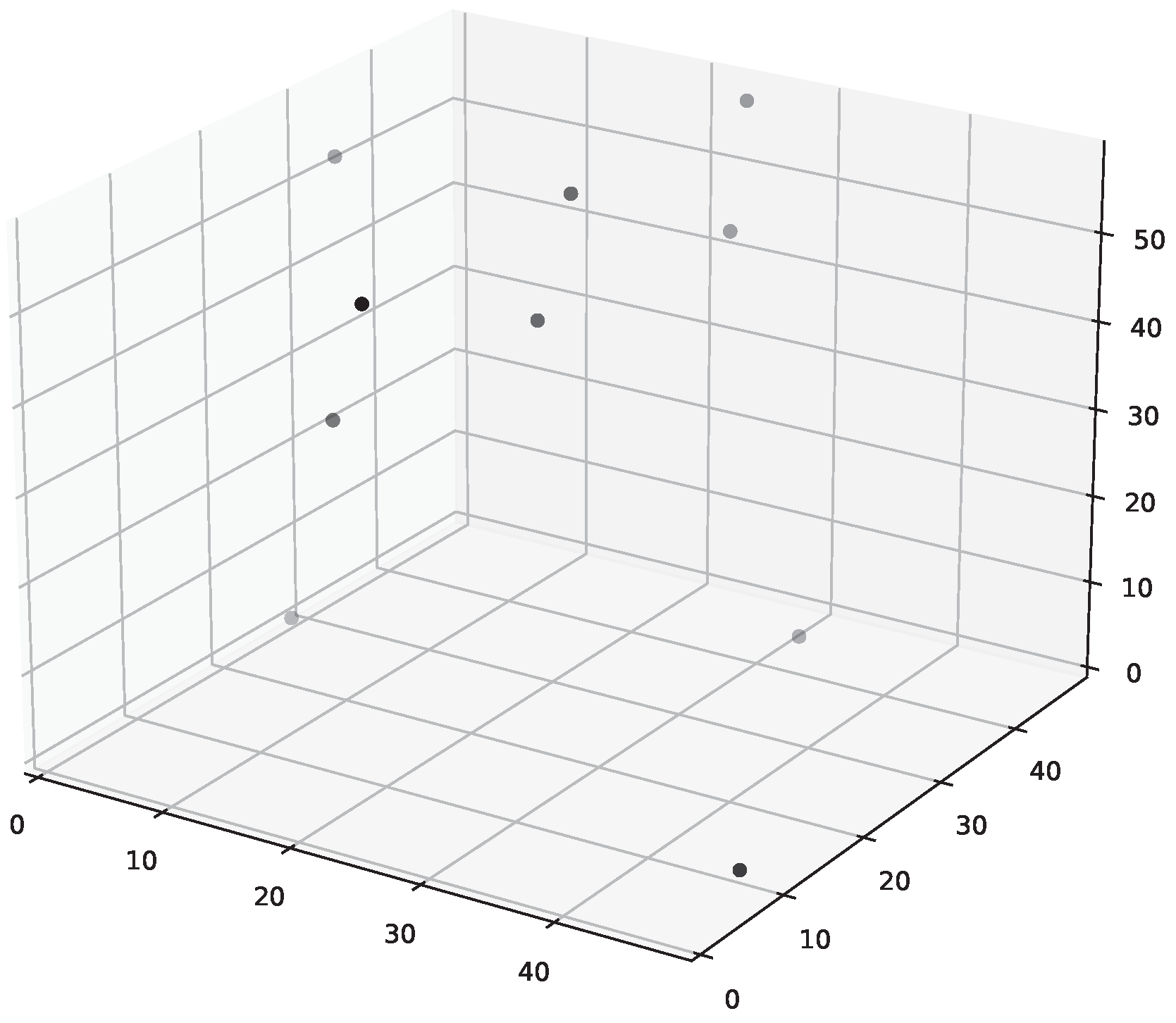
The POD modes of the temperature data from training set were used as the tailored basis. The first two of those dominant temperature POD modes are shown in Figure 3. The POD modes () are then used to find good sensor locations (pivots in C) in the temperature grid, as shown in Figure 4.
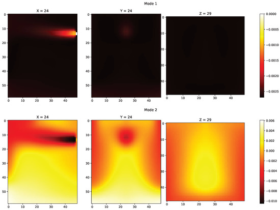
Figure 3.
Mode 1 and Mode 2 from POD decomposition.
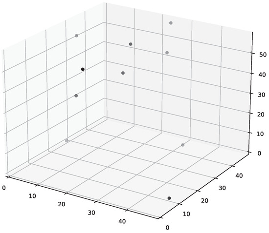
Figure 4.
The chosen sensor locations.
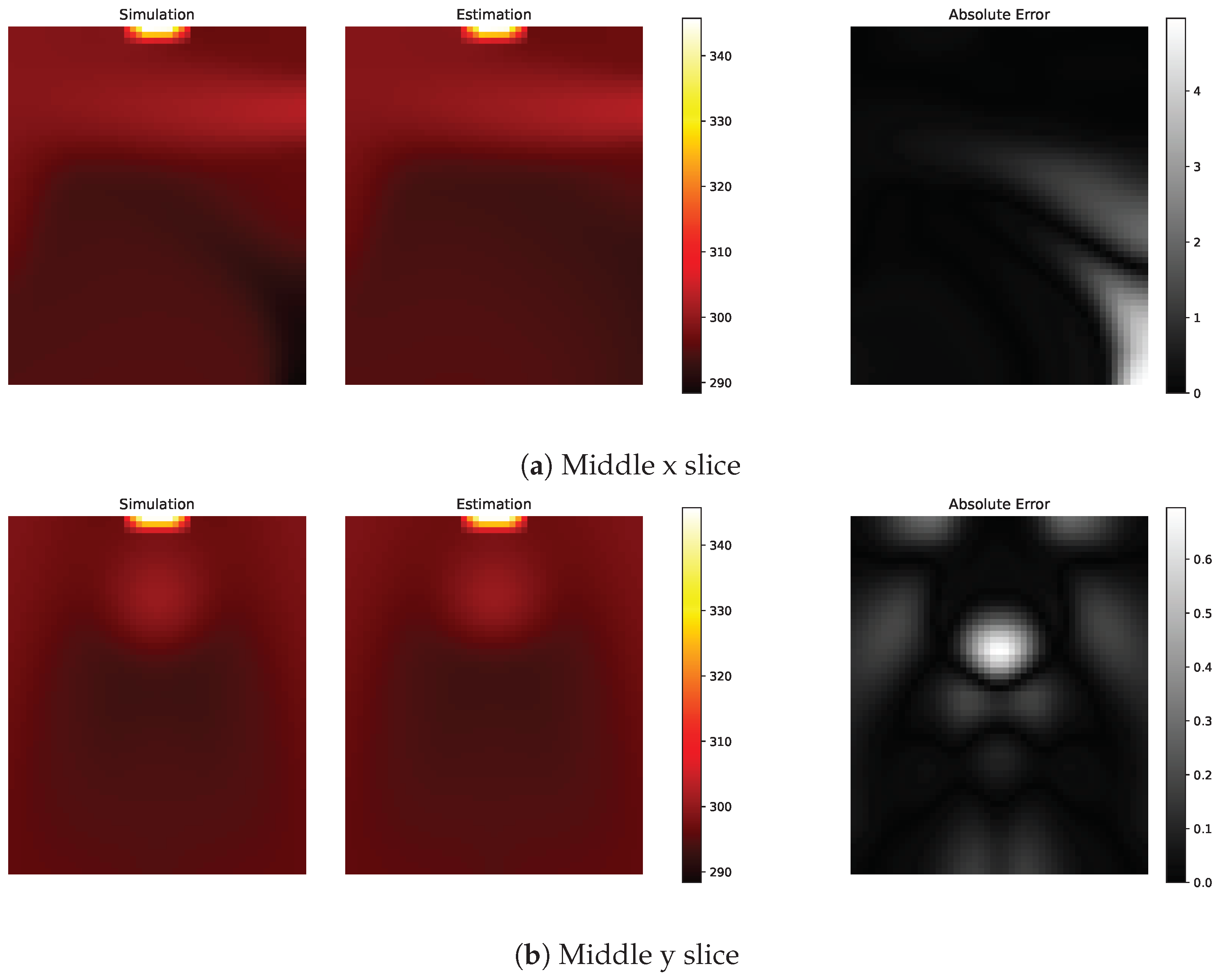
These are the physical locations that should be measured for the reconstruction. Thus, one can estimate the whole temperature grid from a given sparse temperature measurement . The temperatures measured in correspond to the location in the measurement matrix . The sparse sensor locations and basis functions obtained using the training data-set are then used to reconstruct the full temperature field for the unseen test case with an inflow of 2 m/s, and this involves using sparse measurements at test case (2 m/s case) at specified locations for the full temperature field reconstruction. The reconstructed flow field is then compared with the full CFD temperature field for the test case. Figure 5 shows examples of temperature estimations obtained from sparse measurements.

Figure 5.
Comparing simulation data and their estimates from sparse measurements. This is for the time step with the largest MAE. Everything is measured in Kelvin.
Since the data are distributed in a 3D space, it is hard to show the entire estimate; these figures show the x and y slices in the middle of the 3D space. Figure 5a shows an example of one of the worst estimates with errors up to 4 Kelvin in the bottom right corner in Figure 5a. For a time-step with an error close to the average error (figure not shown), there are no errors above 1 K.
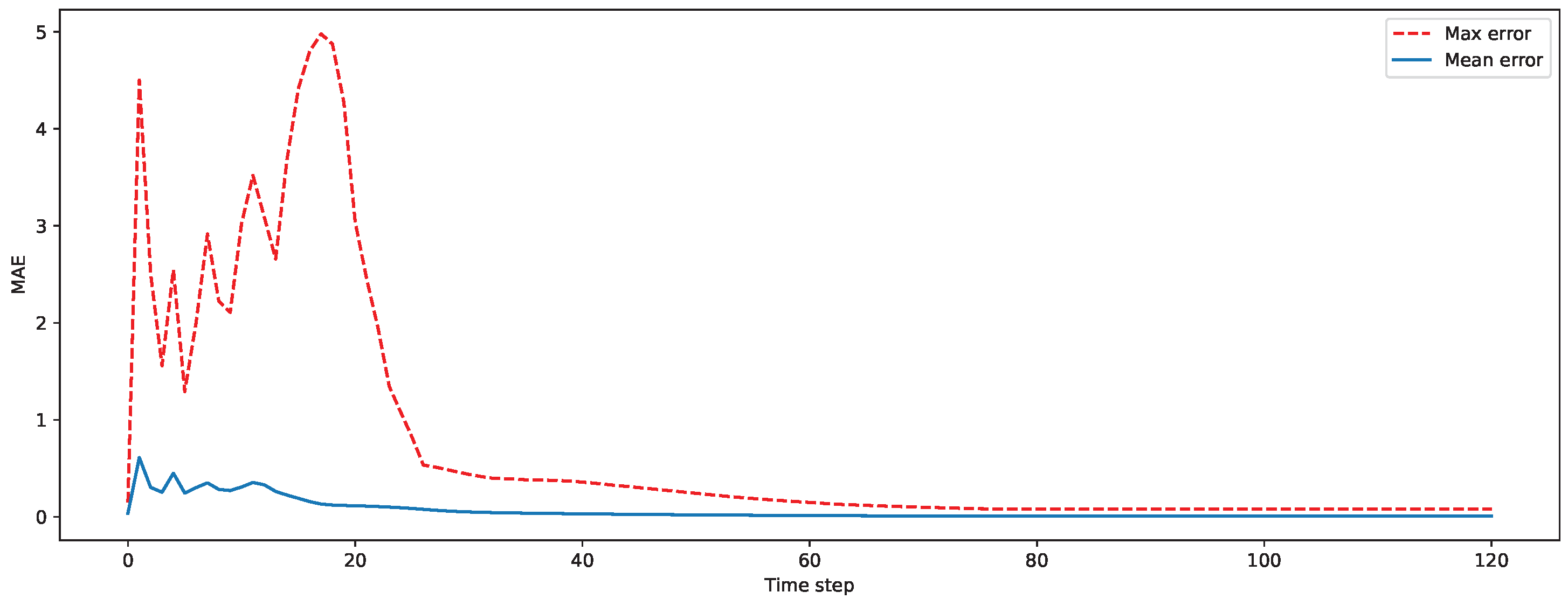
As seen in Figure 6 the error is largest in the first time steps of the time series estimated from sparse measurements. In the beginning of the simulation, the temperature is harder to model than the more homogeneous temperature that dominates the later time steps. The sparse measurements are used to find the linear combination of the POD modes that best fits the current state. If the current temperature field does not fit well with the POD modes, the estimate of the sparse measurement will not provide a result that is close to the ground truth. This is independent of the number of sensor locations that are used, as long as the number of POD modes does not increase.

Figure 6.
Maximum and average absolute error for each time step.
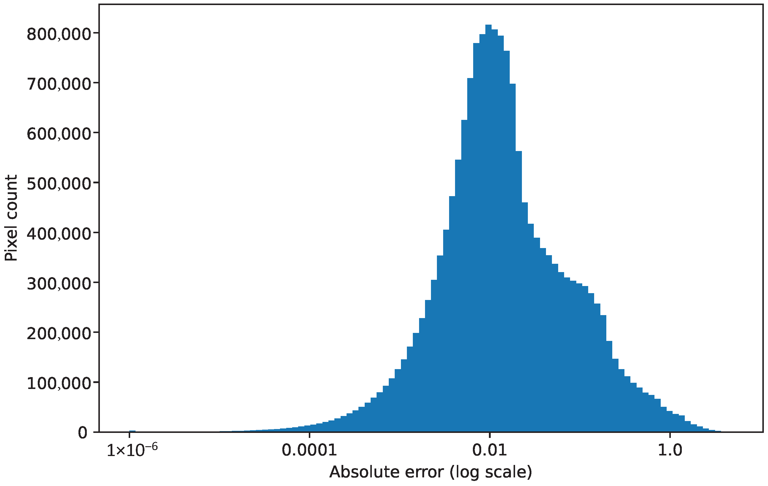
A histogram of all the absolute errors at every spatial location and time step is shown in Figure 7. In this histogram, the vast majority of the errors in temperature estimation are below 0.5 Kelvin. Therefore, there seems to be only a few time steps and spatial positions with large errors, which provide the large errors shown in Figure 5 and Figure 6. The errors are low in the rest of the region. Thus, the flow reconstruction from the sensor can be considered good, with scope for improvements in the future. In next section, we will see results for the reconstruction of a flow field using a data-driven reduced-order model for efficient predictions in a DT set-up.

Figure 7.
Histogram of the absolute error for each pixel for each time step.
3.2. Flow Reconstruction of Velocity Using LSTM-POD ROM
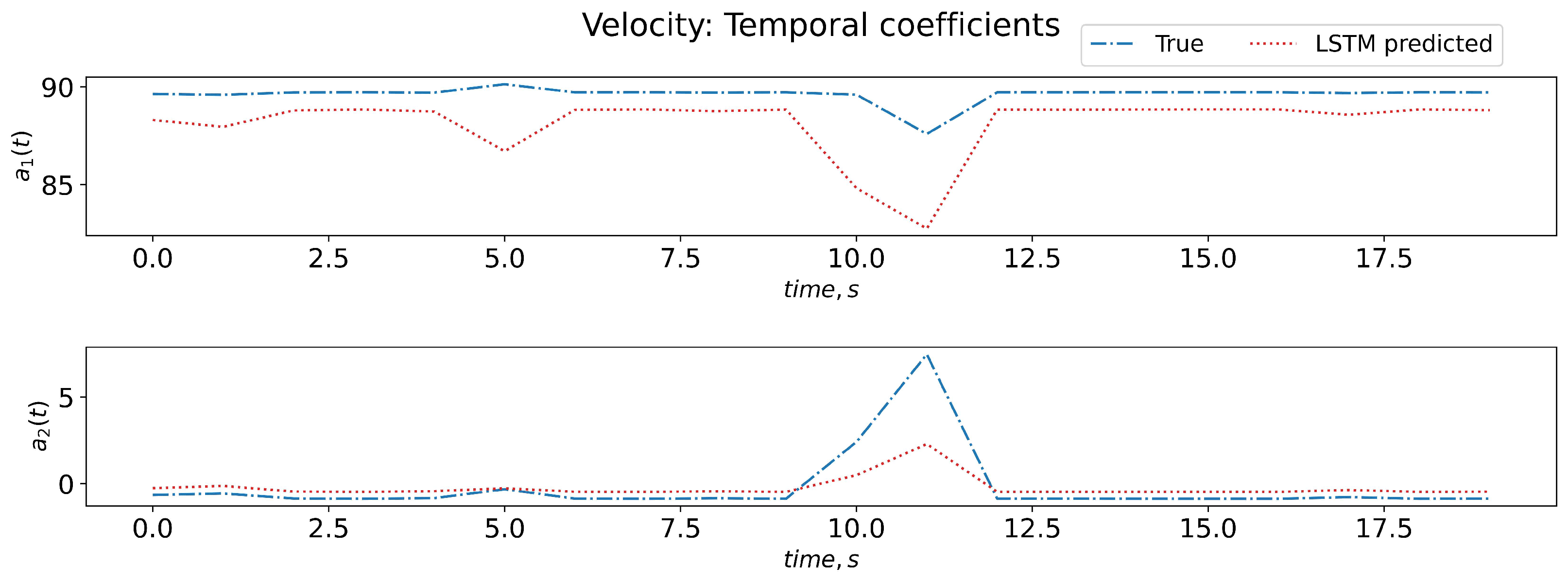
The training data-set for LSTM comprises an input 3D matrix containing the POD-evaluated time-coefficients and has dimensions of , corresponding to the number of samples (N), the look-back time steps ( = 3 for this work) and the number of features (R). The R number of features correspond to the temporal coefficient values associated with R spatial basis function (modes). If needed, the flow-rate can be added as an additional feature (parameter). For LSTM output (target), a database of a 2D array of the temporal coefficients for time t is provided with dimensions to train the LSTM. The LSTM is trained to map the inputs ( previous time-steps of time coefficients) to time-coefficient values at time t for all R modes. Here, the LSTM parameters are found using the hyper-parameter optimization software optuna. The LSTM uses two layers with 30 units (neurons) and tanh activation function. The details of the ROM methodology involving LSTM can be found at [6]. Figure 8 shows the temporal dynamics of coefficients, as predicted by the trained LSTM model on test data. The trained LSTM model could qualitatively predict the temporal coefficient evolution trend when compared to the actual true coefficient. There is scope for improvements in its accuracy when using a larger training database to provide a result that is qualitatively similar to the true coefficient. These temporal coefficients are now used, along with the velocity basis functions (obtained from POD), to reconstruct the full velocity field for the unseen test case (as seen in Figure 9).
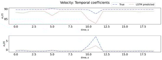
Figure 8.
Temporal dynamics of coefficients captured by LSTM.
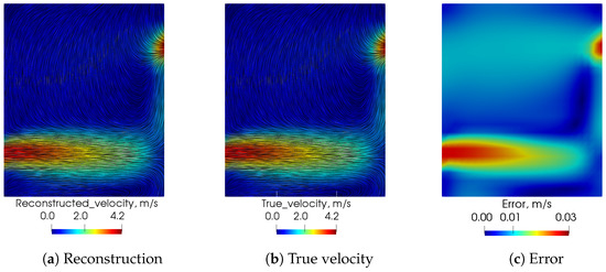
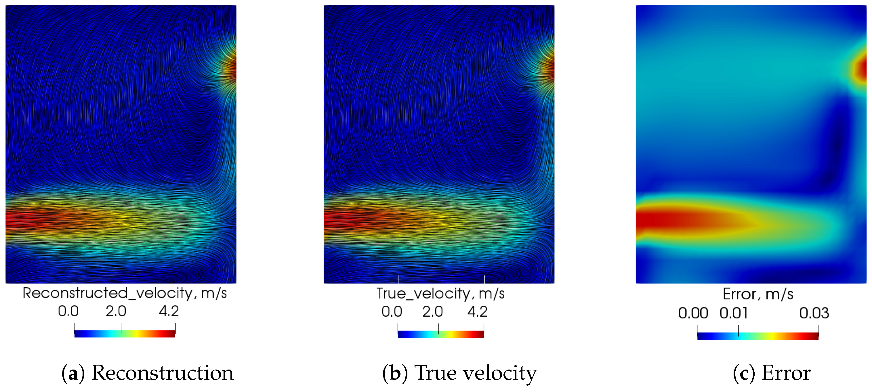
Figure 9.
Comparison of prediction of velocity field between LSTM-POD reconstruction and hi-fidelity CFD.
Figure 9 shows the reconstruction of velocity field at time t before the flow is fully developed using the (a) LSTM-POD methodology compared to that obtained by (b) high-fidelity CFD data.
Figure 9 shows that the LSTM-POD methodology can predict qualitatively similar results (flow field) as actual CFD data in an online set-up using only a few minutes of computational time, as compared to the few hours of computational time needed by the hi-fidelity CFD with minimal errors. Thus, the methodologies developed to date have potential for use in a synthetic CFD data-set. The flow reconstruction from sensors needs to be further tested on actual sensor measurements in the experimental set-up, and there is scope for corrections to the reconstruction errors using techniques such as hybrid analytics and modelling.
4. Conclusions
The application of data-driven optimal temperature sensor placements and reduced-order models enabled us to reconstruct and predict the full-scale temperature and flow field for a synthetic dataset for a greenhouse digital twin set-up. The methodology shows promise in monitoring the spatio-temporal dynamics of key variables for a digital twin greenhouse setup. Future work involves increasing further the accuracy using an HAM-corrective source term approach to correct the reconstruction error while using sparse sensors and reduced-order models, and testing these with actual measurements from the experimental set-up.
Author Contributions
Conceptualization, A.R. and M.T.; methodology and experiments, K.S., E.B., M.T. and A.R.; CFD data curation, M.T.; greenhouse experiments and data curation, E.B.; software, K.S. and M.T.; validation, K.S. and E.B.; formal analysis, K.S. and M.T.; investigation, K.S. and M.T.; resources, A.R.; writing—original draft preparation, K.S., E.B. and M.T.; writing—review and editing, A.R. and M.T.; visualization, M.T., K.S. and E.B.; supervision, A.R. and M.T.; project administration, A.R.; funding acquisition, A.R. and M.T. All authors have read and agreed to the published version of the manuscript.
Funding
This research was funded by the SEP funding from SINTEF for the project named: Highly Capable Digital twin, SEP project number: 102024647-54.
Institutional Review Board Statement
Not applicable.
Informed Consent Statement
Not applicable.
Data Availability Statement
The data can be made available on request.
Acknowledgments
We would like to thank Disruptive Technologies for contributing with their advanced temperature and humidity sensors for the project.
Conflicts of Interest
The authors declare no conflict of interest.
References
- Rasheed, A.; San, O.; Kvamsdal, T. Digital Twin: Values, Challenges and Enablers from a modeling perspective. IEEE Access 2020, 8, 21980–22012. [Google Scholar] [CrossRef]
- Donoho, D. Compressed sensing. IEEE Trans. Inf. Theory 2006, 52, 1289–1306. [Google Scholar] [CrossRef]
- Manohar, K.; Brunton, B.W.; Kutz, J.N.; Brunton, S.L. Data-Driven Sparse Sensor Placement for Reconstruction: Demonstrating the Benefits of Exploiting Known Patterns. IEEE Control Syst. Mag. 2018, 38, 63–86. [Google Scholar] [CrossRef]
- Pawar, S.; Ahmed, S.E.; San, O.; Rasheed, A. Data-driven recovery of hidden physics in reduced order modeling of fluid flows. Phys. Fluids 2020, 32, 036602. [Google Scholar] [CrossRef]
- Ahmed, S.E.; Pawar, S.; San, O.; Rasheed, A.; Tabib, M. A nudged hybrid analysis and modeling approach for realtime wake-vortex transport and decay prediction. Comput. Fluids 2021, 221, 104895. [Google Scholar] [CrossRef]
- Tabib, M.V.; Pawar, S.; Ahmed, S.E.; Rasheed, A.; San, O. A non-intrusive parametric reduced order model for urban wind flow using deep learning and Grassmann manifold. J. Phys. Conf. Ser. 2021, 2018, 012038. [Google Scholar] [CrossRef]

Disclaimer/Publisher’s Note: The statements, opinions and data contained in all publications are solely those of the individual author(s) and contributor(s) and not of MDPI and/or the editor(s). MDPI and/or the editor(s) disclaim responsibility for any injury to people or property resulting from any ideas, methods, instructions or products referred to in the content. |
© 2023 by the authors. Licensee MDPI, Basel, Switzerland. This article is an open access article distributed under the terms and conditions of the Creative Commons Attribution (CC BY) license (https://creativecommons.org/licenses/by/4.0/).