Proceeding Paper

Sensor Virtualization for Anomaly Detection of Turbo-Machinery Sensors—An Industrial Application †

1
Baker Hughes, Doddanakundi Industrial Area 2, Bengaluru 560037, India
2
Baker Hughes (Nuovo Pignone Tecnologie), Via Felice Matteucci 2, 50127 Firenze, Italy
*
Authors to whom correspondence should be addressed.
Presented at the 9th International Conference on Time Series and Forecasting, Gran Canaria, Spain, 12–14 July 2023.
Eng. Proc. 2023, 39(1), 96; https://doi.org/10.3390/engproc2023039096
Published: 27 July 2023
(This article belongs to the Proceedings of The 9th International Conference on Time Series and Forecasting)

Abstract

:
We apply a Granger causality and auto-correlation analysis to train a recurrent neural network (RNN) that acts as a virtual sensor model. These models can be used to check the status of several hundreds of sensors during turbo-machinery units’ operation. Checking the health of each sensor is a time-consuming activity. Training a supervised algorithm is not feasible because we do not know all the failure modes that the sensors can undergo. We use a semi-supervised approach and train an RNN (LSTM) on non-anomalous data to build a virtual sensor using other sensors as regressors. We use the Granger causality test to identify the set of input sensors for a given target sensor. Moreover, we look at the auto-correlation function (ACF) to understand the temporal dependency in data. We then compare the predicted signal vs. the real one to raise (in case) an anomaly in real time. Results report 96% precision and 100% recall.

1. Introduction

Turbo-machinery units are equipped with hundreds of sensors to monitor their health during functioning [1,2]. Some of these sensors measure primary physical quantities, which can affect the overall health of the machine. Thus, detecting the improper behavior of sensors or mechanical equipment is a critical task in energy [3,4] and the mechanical industry or, generally speaking, in every IOT-related industry [5]. Detecting unexpected behavior is also a challenging task [2,6]; indeed, in many real-world problems, samples from the unexpected classes are of insufficient sizes to be effectively modeled using supervised algorithms [7]. Anomaly detection identifies novelty cases by training only on samples considered normal and then identifying the unusual cases [8,9,10].

1.1. Problem Statement

In this domain, monitoring some sensors is important because they can trigger alerts; in that case, a machine shutdown and manual inspections are required, with an associated cost. Sometimes the triggers are false since they are caused by a sensor failure, not by a machine issue. Hence, early detection is required to avoid undesired shutdowns. Indeed, if a sensor is about to break, service operations can exclude this sensor from the control strategy.
We want to detect possible faults (anomalies) in the sensors installed on our turbo machines (Figure 1) to prevent unnecessary inspection/shutdown efforts by site engineering while making sure that correct triggers, instead, are not ignored.
The challenge consists in dealing with these aspects:
  • Early detection is required: only a prompt action allows to avoid the high potential costs of unnecessary shutdowns.
  • Up to few thousand sensors need to be checked daily.
  • Recall is key: anomalies detected by the tool will be checked by operators and vice versa, where if no alert is given, the anomaly may remain undetected.
  • Precision should be kept under control: too many false positives would increase the set of signals to be checked and may invalidate the benefits.

1.2. Related Works

Many other authors have tried to solve similar problems with different techniques: Malhotra et al. [11] apply recurrent neural networks (RNNs) for anomaly detection on aircraft. Park et al. [12] and Pereira [13] uses variational recurrent autoencoder and clustering to detect anomalous time series in healthcare. Geiger et al. [14] applies generative adversarial networks (GANs) and LSTM to identify the temporal correlations of time-series distributions (see also [15,16]). Zheng et al. [17] apply long short-term memory for residual useful life estimation. In a similar research, Strazzera et al. [1] confirm that LSTM outperforms the not recurrent neural network also in the domain adaptation. Zhang et al. [18] extend reinforcement learning (RL) and the Markov decision process [19] to build a general framework for fault prediction and residual useful life estimation. Several other authors (Yang [20], Pawełczyk and Sepe [21]) use machine-learning-based prediction models for gas turbine operating parameters estimation (see also [22] for a small review). They find that machine learning techniques are applicable to any of the gas turbine parameters when reference physics-based models and large sensor measurements datasets are available to validate the accuracy of the data-driven algorithms developed. Escobedo [23] uses the Bayesian technique and feature extraction to scale up to a broad large mechanical equipment fleet.

2. The Dataset

Our data are output from all sensors installed on a turbo machine [1,2] and are acquired at a frequency of one sample per second. Different kinds of sensors like temperature, pressure, speed sensors have been acquired and comprise our database. Among these sensors, the ones which are critical for machine control are considered “output sensors” in our work. In fact, those are the sensors whose health needs to be monitored to be sure that an eventual alarm triggered by them is actually due to a machine failure, not to a probe failure. The remaining sensors can be used as input features for building virtual sensor models (digital twins) of the first set of sensors. In this work, we focus on one target sensor only to explain the process more easily.
The dataset was collected during 14 months of machine operation (1 s sampling interval). It was split into training (10 months data), validation (1 month data) and test (3 months data) sets. The training data have no reported anomaly, while the validation and test sets have some anomalies reported.

3. The Model

3.1. Selection of Input Sensors

There are more than 200 sensors that can be used to build a virtual sensor for each output sensor. We used the Granger Causality [24,25] test to determine the subset of input sensors that have a causal effect on the target. For the target sensor shown here, we identified around 15 input sensors to be used to reconstruct the same.

3.2. Selection of Lookback Window

We used the auto-correlation to find the temporal relations in both input sensors and target sensor to obtain the best “window size” to train the LSTM model.
Figure 2a shows the auto-correlation function (ACF) graph for one of the sensors: we can see high correlation values among all the lags, which represent the presence of strong trend (non-stationary series). Hence, we need to make this series stationary by differentiating to view if there is any seasonality present in the data.
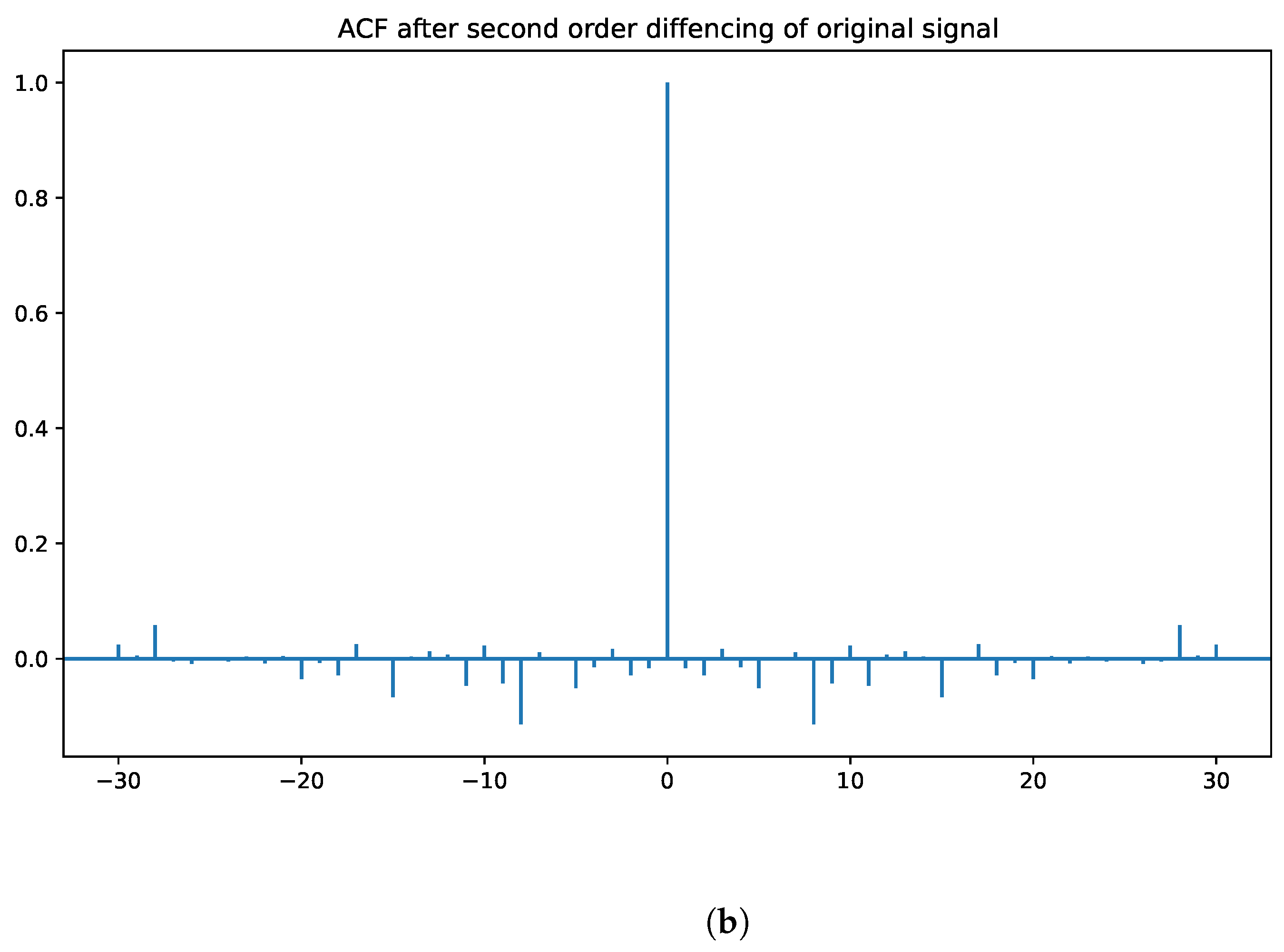
Figure 2b shows the auto-correlation function (ACF) graph after second-order differentiation: there is no significant seasonality and a small degree of trend. Thus, we can conclude the absence of seasonality but the presence of strong trend (strong correlation among first few lag values). Moreover, we know from subject matter experts that in turbo-machinery applications the thermocouple thermal inertia is less than 5 s [26]. Hence, we chose a sliding window of five samples for this temperature-measuring sensor selected as output. Indeed, after five samples, ACF shows highly sparse values.

3.3. Model Training

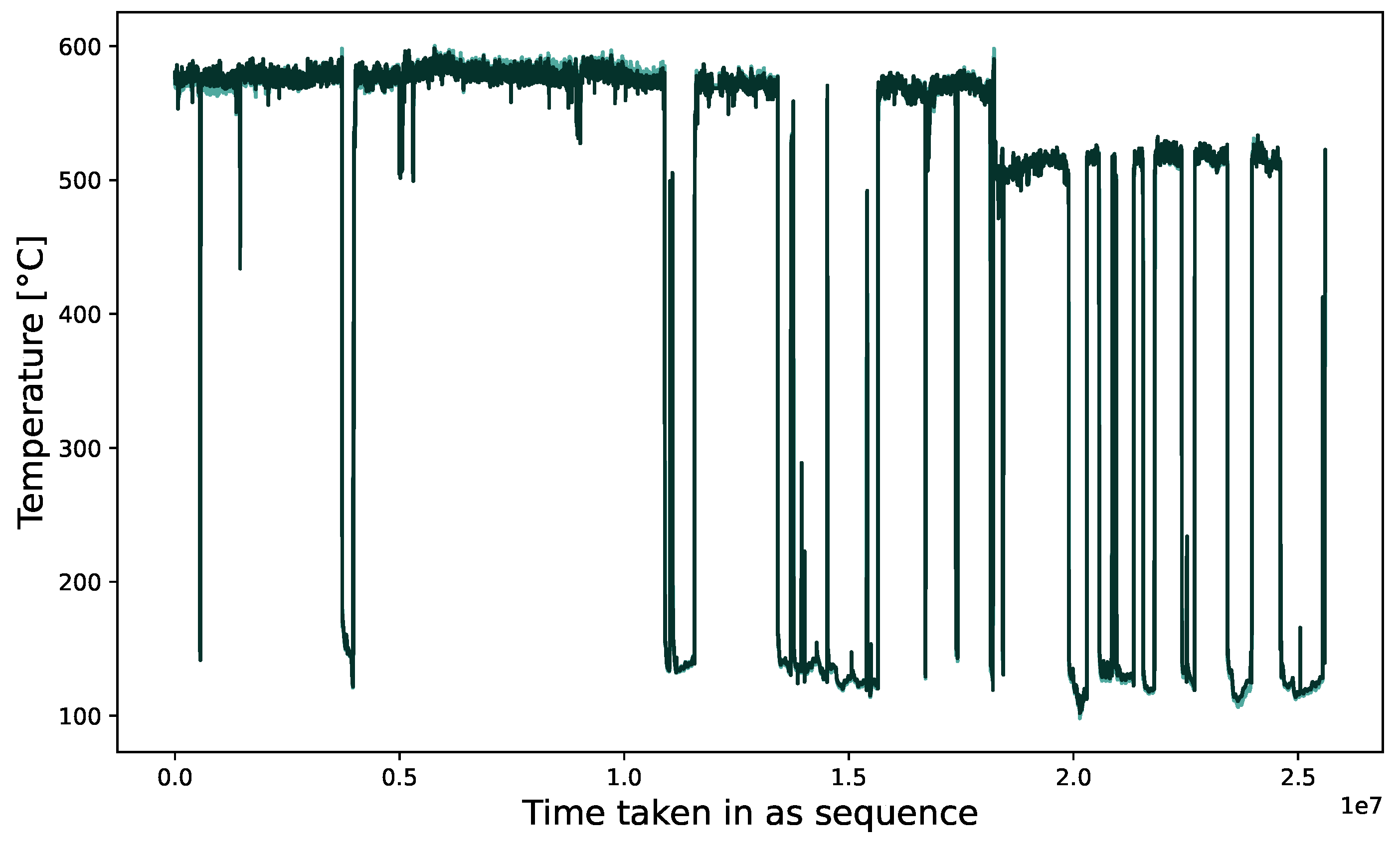
We used a deep learning model with two long short-term memory (LSTM) layers of 32 nodes each, with tanh activation, followed by four fully connected layers with ReLU activation. We used Adam optimizer to train the model and a callback on the validation set to stop the training. We used a semi-supervised [2] approach and trained the model on non-anomalous data only to build a virtual sensor acting like a digital twin of the sensor itself [11,27]. In Figure 3, we can see that the model is able to correctly reproduce the actual signal.

3.4. Inference Logic

Once the model has been trained, we use it to reconstruct the signal in a time region when sensor anomalies may have occurred. To distinguish between anomalous and non-anomalous samples, we identified a criterion based on the level of agreement of the actual sensor with respect to the virtual one.
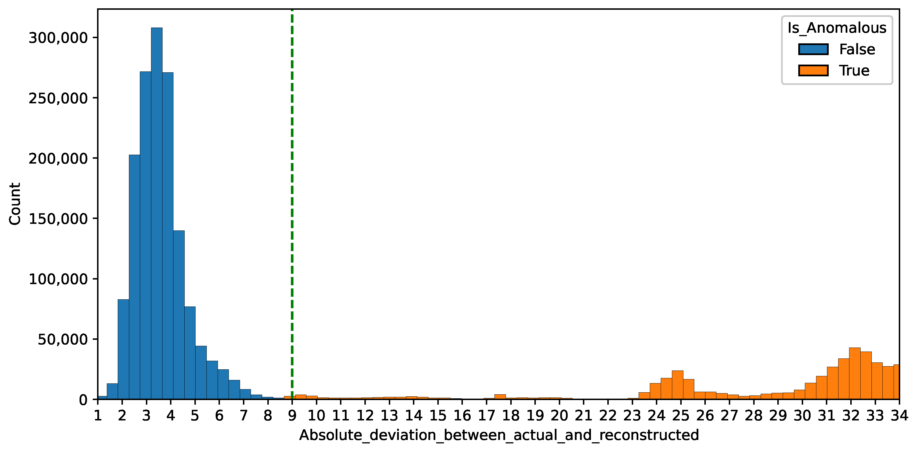
Given the actual signal y i , with i = 0 , , T , where T is the signal length, and the related virtual signal y i ^ , with i = 0 , , T , the discrepancy Δ y i = a b s ( y i ^ y i ) , i = 0 , , T can be calculated. We declare y i to be anomalous if its related Δ y i is higher than expected. This expected value was derived by looking at the values of Δ y i of non-anomalous samples in the validation set. Furthermore, given that the validation set contains both anomalous and non-anomalous samples, we leveraged the different Δ y i distribution between non-anomalous and anomalous samples to determine the threshold value. Figure 4 shows the distribution of the discrepancy Δ y i , i = 0 , , T v , where T v is the validation set length in the case of anomalous (orange) and non-anomalous (blue) points.
In this example, we can see two non-overlapping distributions: here, we decided to use a threshold of 9 to best discriminate between anomalous and non-anomalous samples.
Another possibility is to leverage the ROC curve to identify the optimal value for the threshold that optimally balances the true positive and false positive rate.
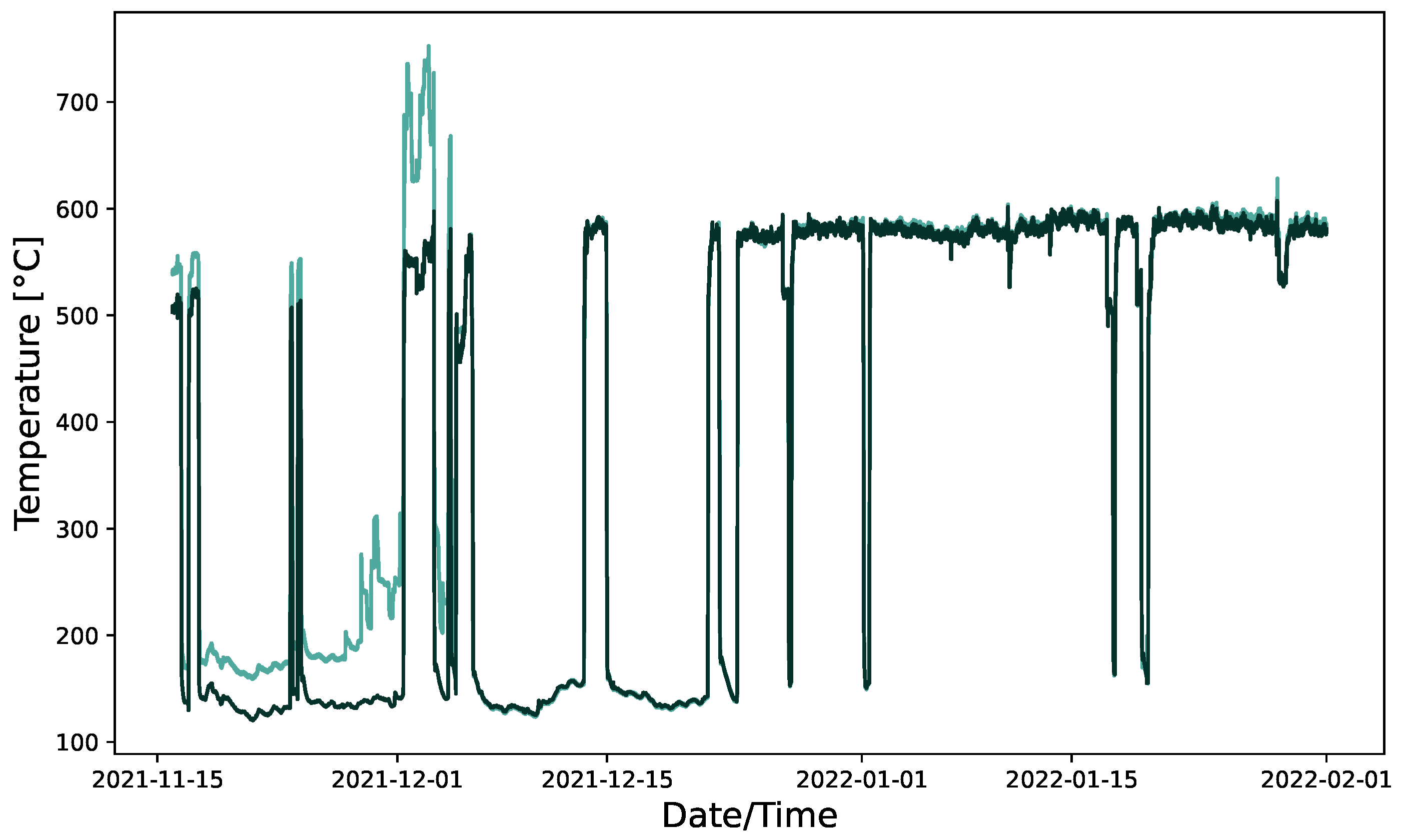
Figure 5 shows the model performance at test time. We can see a good agreement between the actual and the virtual signal in the region where no sensor anomalies occurred (rightmost part of the plot) and, instead, a discrepancy between them in a region where sensor anomalies are present (leftmost part of the plot).

4. Results

Table 1 shows the reconstruction performance of the model on training, validation and test sets. For validation and test sets, the metrics are evaluated only using subsets where no anomalies occurred. Please note that the error Δ is defined here as the deviation between the actual signal y and the reconstructed signal y ^ : Δ = y y ^ , then ME is the mean error, MAPE is the mean absolute percentage error, and P90 is the 90th percentile of the absolute value of the error Δ .
For what concerns the anomaly detection performance, when applying the model to the test set, we are able to detect anomalous signals with 96% precision and 100% recall as summarized in Table 2.

5. Conclusions

In this work, we presented a real industrial application of sensor anomaly detection in the domain of energy and turbomachinery. We applied a semi-supervised deep learning technique, which can be used to perform anomaly detection in an industrial context. In particular, we applied anomaly detection to turbo-machinery units by training a virtual sensor model for a given sensor. We first selected input features through Granger causality and leveraged auto-correlation and subject matter expertise to identify the best window size for the recurrent neural network chosen (LSTM).
This method can be scaled and extended to almost all the sensors installed on the unit, for a complete sensor anomaly detection system.
Furthermore, once the model has been trained for a single sensor, we can later retrain the model using data collected over time, with a continual learning approach [28] so that the algorithm is able to also take into account data-shift phenomena.
Our next plans focus on the deployment of the inference algorithm on edge devices, i.e., on the MarkVIe system. For this purpose, some model distillation may be required (for a review, see [29]). In particular, we need to detect potential sensor faults as early as possible so that we can exclude the sensor from the control system, thus avoiding undesired shutdowns.

Author Contributions

S.S. and V.G.: developed the model; G.B. defined the problem and data analysis; G.V. reviewed the model and contributed to model definition and performance analysis. All authors have read and agreed to the published version of the manuscript.

Funding

This research received internal funding.

Institutional Review Board Statement

Baker Hughes internal review process: # 1440.

Informed Consent Statement

Authors authorize the use and disclosure of the following information for this research.

Data Availability Statement

Proprietary Data.

Acknowledgments

Thanks to Luca Strazzera, Andrea Panizza and Laure Barrière for the valuable discussion.

Conflicts of Interest

The authors declare no conflict of interest.

References

  1. Strazzera, L.; Gori, V.; Veneri, G. DANNTe: A Case Study of a Turbo-Machinery Sensor Virtualization under Domain Shift. arXiv 2021, arXiv:2201.03850. [Google Scholar]
  2. Gori, V.; Veneri, G.; Ballarini, V. Continual Learning for anomaly detection on turbomachinery prototypes—A real application. In Proceedings of the 2022 IEEE Congress on Evolutionary Computation (CEC), Padua, Italy, 18–23 July 2022; pp. 1–7. [Google Scholar] [CrossRef]
  3. Michelassi, V.; Allegorico, C.; Cioncolini, S.; Graziano, A.; Tognarelli, L.; Sepe, M. Machine Learning in Gas Turbines. Mech. Eng. 2018, 140, S54–S55. [Google Scholar] [CrossRef] [Green Version]
  4. Wu, Y.; Yuan, M.; Dong, S.; Lin, L.; Liu, Y. Remaining useful life estimation of engineered systems using vanilla LSTM neural networks. Neurocomputing 2018, 275, 167–179. [Google Scholar] [CrossRef]
  5. Capasso, A. Hands-On Industrial Internet of Things: Create a Powerful Industrial IoT Infrastructure Using Industry 4.0; Packt Publishing: Birmingham, UK, 2018. [Google Scholar]
  6. Hodge, V.J.; Austin, J. A Survey of Outlier Detection Methodologies. Artif. Intell. Rev. 2004, 22, 85–126. [Google Scholar] [CrossRef] [Green Version]
  7. Zimek, A.; Schubert, E.; Kriegel, H.P. A survey on unsupervised outlier detection in high-dimensional numerical data. Stat. Anal. Data Mining Asa Data Sci. J. 2012, 5, 363–387. [Google Scholar] [CrossRef]
  8. Akcay, S.; Atapour-Abarghouei, A.; Breckon, T.P. GANomaly: Semi-Supervised Anomaly Detection via Adversarial Training. arXiv 2018, arXiv:cs.CV/1805.06725. [Google Scholar]
  9. Akçay, S.; Atapour-Abarghouei, A.; Breckon, T.P. Skip-GANomaly: Skip Connected and Adversarially Trained Encoder-Decoder Anomaly Detection. arXiv 2019, arXiv:cs.CV/1901.08954. [Google Scholar]
  10. Nanduri, A.; Sherry, L. Anomaly detection in aircraft data using Recurrent Neural Networks (RNN). In Proceedings of the 2016 Integrated Communications Navigation and Surveillance (ICNS), Herndon, VA, USA, 19–21 April 2016; pp. 5C2–1–5C2–8. [Google Scholar]
  11. Malhotra, P.; Vig, L.; Shroff, G.M.; Agarwal, P. Long Short Term Memory Networks for Anomaly Detection in Time Series. In Proceedings of the 23rd European Symposium on Artificial Neural Networks, Computational Intelligence and Machine Learning, (ESANN 2015), Bruges, Belgium, 22–24 April 2015; pp. 89–94. [Google Scholar]
  12. Park, D.; Hoshi, Y.; Kemp, C.C. A Multimodal Anomaly Detector for Robot-Assisted Feeding Using an LSTM-Based Variational Autoencoder. IEEE Robot. Autom. Lett. 2018, 3, 1544–1551. [Google Scholar] [CrossRef] [Green Version]
  13. Pereira, J.; Silveira, M. Learning Representations from Healthcare Time Series Data for Unsupervised Anomaly Detection. In Proceedings of the 2019 IEEE International Conference on Big Data and Smart Computing (BigComp), Kyoto, Japan, 27 February–2 March 2019; pp. 1–7. [Google Scholar]
  14. Geiger, A.; Liu, D.; Alnegheimish, S.; Cuesta-Infante, A.; Veeramachaneni, K. TadGAN: Time Series Anomaly Detection Using Generative Adversarial Networks. In Proceedings of the 2020 IEEE International Conference on Big Data (Big Data), Osaka, Japan, 17–20 December 2022; pp. 33–43. [Google Scholar] [CrossRef]
  15. Li, Y.; Peng, X.; Zhang, J.; Li, Z.; Wen, M. DCT-GAN: Dilated Convolutional Transformer-based GAN for Time Series Anomaly Detection. IEEE Trans. Knowl. Data Eng. 2021, 35, 3632–3644. [Google Scholar] [CrossRef]
  16. Sabuhi, M.; Zhou, M.; Bezemer, C.P.; Musilek, P. Applications of Generative Adversarial Networks in Anomaly Detection: A Systematic Literature Review. IEEE Access 2021, 9, 161003–161029. [Google Scholar] [CrossRef]
  17. Zheng, S.; Ristovski, K.; Farahat, A.; Gupta, C. Long Short-Term Memory Network for Remaining Useful Life estimation. In Proceedings of the 2017 IEEE International Conference on Prognostics and Health Management (ICPHM), Dallas, TX, USA, 19–21 June 2017; pp. 88–95. [Google Scholar]
  18. Zhang, C.; Gupta, C.; Farahat, A.; Ristovski, K.; Ghosh, D. Equipment Health Indicator Learning Using Deep Reinforcement Learning. In Proceedings of the Machine Learning and Knowledge Discovery in Databases; Brefeld, U., Curry, E., Daly, E., MacNamee, B., Marascu, A., Pinelli, F., Berlingerio, M., Hurley, N., Eds.; Springer: New York, NY, USA, 2019; pp. 488–504. [Google Scholar]
  19. Jacobs, W.R.; Edwards, H.; Li, P.; Kadirkamanathan, V.; Mills, A.R. Gas turbine engine condition monitoring using Gaussian mixture and hidden Markov models. Int. J. Progn. Health Manag. 2018, 9, 1–15. [Google Scholar] [CrossRef]
  20. Yang, C.; Gunay, B.; Shi, Z.; Shen, W. Machine Learning-Based Prognostics for Central Heating and Cooling Plant Equipment Health Monitoring. IEEE Trans. Autom. Sci. Eng. 2020, 18, 346–355. [Google Scholar] [CrossRef]
  21. Pawełczyk, V.; Fulara, S.; Sepe, M.; De Luca, A.; Badora, M. Industrial gas turbine operating parameters monitoring and data-driven prediction. Eksploat. I Niezawodn. 2020, 22, 391–399. [Google Scholar] [CrossRef]
  22. Yan, Z.; Sun, J.; Yi, Y.; Yang, C.; Sun, J. Data-Driven Anomaly Detection Framework for Complex Degradation Monitoring of Aero-Engine. Int. J. Turbomach. Propuls. Power 2023, 8, 3. [Google Scholar] [CrossRef]
  23. Ernesto Escobedo, E.; Arguello, L.; Sepe, M.; Parrella, I.; Cioncolini, S.; Allegorico, C. Enhanced early warning diagnostic rules for gas turbines leveraging on bayesian networks. In Proceedings of the ASME Turbo Expo 2020: Turbomachinery Technical Conference and Exposition, Virtual, 21–25 September 2020. [Google Scholar]
  24. Granger, C. Investigating Causal Relations by Econometric Models and Cross-Spectral Methods. Econometrica 1969, 37, 424–438. [Google Scholar] [CrossRef]
  25. Rosoł, M.; Młyńczak, M.; Cybulski, G. Granger causality test with nonlinear neural-network-based methods: Python package and simulation study. Comput. Methods Programs Biomed. 2022, 216, 106669. [Google Scholar] [CrossRef]
  26. Straubinger, D.; Illés, B.; Busek, D.; Codreanu, N.; Géczy, A. Modelling of thermocouple geometry variations for improved heat transfer monitoring in smart electronic manufacturing environment. Case Stud. Therm. Eng. 2022, 33, 102001. [Google Scholar] [CrossRef]
  27. Tran, K.P.; Nguyen, H.D.; Thomassey, S. Anomaly detection using Long Short Term Memory Networks and its applications in Supply Chain Management. IFAC-PapersOnLine 2019, 52, 2408–2412. [Google Scholar] [CrossRef]
  28. Rebuffi, S.A.; Kolesnikov, A.; Sperl, G.; Lampert, C.H. iCaRL: Incremental Classifier and Representation Learning. arXiv 2017, arXiv:cs.CV/1611.07725. [Google Scholar]
  29. Gou, J.; Yu, B.; Maybank, S.J.; Tao, D. Knowledge Distillation: A Survey. Int. J. Comput. Vis. 2021, 129, 1789–1819. [Google Scholar] [CrossRef]
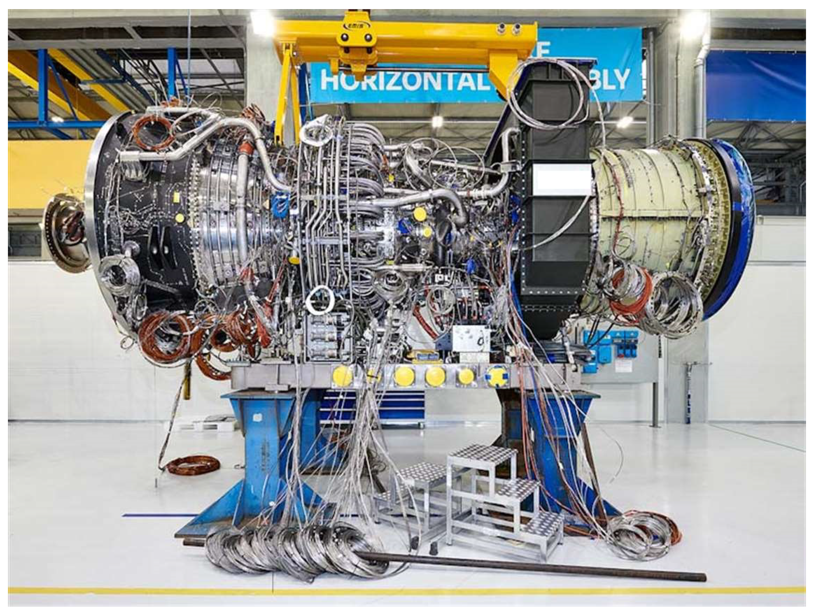
Figure 1. Turbine: a turbo machine is a system that transfers energy between a rotor and a fluid, including both turbines and compressors. While a turbine transfers energy from a fluid to a rotor, a compressor transfers energy from a rotor to a fluid.
Engproc 39 00096 g001
Figure 2. (a) Auto-correlation function plot for one of target sensor. (b) Auto-correlation function plot after second-order derivative to make series stationary.
Engproc 39 00096 g002aEngproc 39 00096 g002b
Figure 3. The picture shows the good fitting between the virtual sensor (dark green) and the actual sensor (light green) for the training set. Values were arbitrarily scaled to maintain data confidentiality.
Engproc 39 00096 g003
Figure 4. Deviation between the actual and the reconstructed signal in the validation set for anomalous (orange) and non-anomalous (blue) samples.
Engproc 39 00096 g004
Figure 5. The picture shows the superposition of the actual signal (light green) and the reconstructed one (dark green). The region ranging from mid November to early December shows a discrepancy between the two: here, a sensor anomaly is highlighted by the model and confirmed by subject matter experts (SMEs). The remaining part of the test set shown here has no anomalies highlighted by the model nor by SMEs. Values were arbitrarily scaled to maintain data confidentiality.
Engproc 39 00096 g005
Table 1. Model performance on training, validation and test sets.
MEMAPEP90
Training set0.120.615.06
Validation set (non-anomalous samples only)1.451.615.97
Test set (non-anomalous samples only)1.890.656.52
Table 2. Anomaly detection performance on the test set.
PrecisionRecall
Full test set96%100%
Disclaimer/Publisher’s Note: The statements, opinions and data contained in all publications are solely those of the individual author(s) and contributor(s) and not of MDPI and/or the editor(s). MDPI and/or the editor(s) disclaim responsibility for any injury to people or property resulting from any ideas, methods, instructions or products referred to in the content.