Long Lead ENSO Forecast Using an Adaptive Graph Convolutional Recurrent Neural Network ^†

Abstract

El Niño-Southern Oscillation (ENSO), a natural phenomenon in the Pacific Ocean, is caused by cyclic changes in sea-surface temperature (SST) and the overlying atmosphere in the tropical Pacific. The impact of ENSO varies, ranging from slightly warmer or colder temperatures to extreme weather events such as flash floods, droughts, and hurricanes, affecting various regions around the globe. Therefore, ENSO forecasting has paramount importance in the atmospheric and oceanic sciences. The Oceanic Niño Index (ONI), a three-month running mean of SST anomalies over the east–central equatorial Pacific region, is the commonly used metric for measuring ENSO events. However, the literature shows that the forecasting accuracy of ONI for lead times exceeding one year is low. This study aims to improve the forecast accuracy of ONI for up to 18 months lead time by applying an Adaptive Graph Convolutional Recurrent Neural Network (AGCRNN). The graph-learning module adaptively learns the spatial structure of features during training, while the graph convolution in hidden layers of the recurrent neural network captures the temporal relationships of features with ONI. Experiments conducted on simulation and reanalysis datasets demonstrate that AGCRNN outperforms state-of-art statistical and eight dynamical models for forecasting ONI with up to 18 months’ lead time.

1. Introduction

El Niño-Southern Oscillation (ENSO) represents the climate variability in the tropical Pacific Ocean caused by coupled ocean–atmosphere interactions and is associated with severe rainfalls, floods, and droughts affecting both tropics and subtropics [1,2]. El Niño in ENSO refers to the periodic warming of sea-surface temperature (SST) across the central and east–central Equatorial Pacific Ocean. Southern Oscillation in ENSO refers to the atmospheric component coupled with sea-surface temperature changes. The warm phase of ENSO is known as El Niño, and the cold phase of ENSO is known as La Niña.

The commonly used metric for measuring ENSO events is the Oceanic Niño Index (ONI). This is a three-month running mean of SST anomalies over the east–central equatorial Pacific region (aka Niño 3.4 region) spanning between 5° N–5° S and 120° W–170° W. An El Niño event is observed in the Niño 3.4 region if the ONI is +0.5 °C or higher, which means that surface waters in the east–central equatorial Pacific are warmer than average by +0.5 °C or higher for five consecutive months. Conversely, a La Niña event is observed in Nino 3.4 region if the ONI is −0.5 °C or lower, which means that surface waters in the east–central equatorial Pacific are colder than average by −0.5 °C or lower for five consecutive months.

ENSO has a profound impact on global climate, with different impacts observed for the warm (El Niño) and the cold phases (La Niña) of ENSO and the region being considered [3,4]. For instance, El Niño is typically linked with warm and dry conditions in the southeastern areas of Australia, Indonesia, the Philippines, and the central Pacific Islands. Furthermore, prolonged El Niño episodes have caused droughts in India, Indonesia, and Australia, and flash floods in the southern United States [5]. In contrast, La Niña is often associated with wetter conditions in eastern Australia and severe rainfall in Indonesia, the Philippines, and Thailand. Coastal Ecuador and northwestern Peru experience drier than average conditions during La Niña. The prolonged La Niña episodes have caused severe rainfall in India, Indonesia, and Australia and droughts in the southern United States [6]. The impacts differ for the two opposite phases of ENSO and their evolutionary patterns. For example, the transition from El Niño to La Niña or La Niña to El Niño caused flash floods in the northeast regions of Asia. Overall, understanding the impact of ENSO events is essential to predicting weather patterns and mitigating the risk of natural disasters.

The conventional approach to machine learning (ML) involves using the input features of each observation to predict the output, which, in this case, determines ONI. However, these features alone are insufficient for spatial–temporal (ST) prediction problems since time and location are critical factors. In addition, forecasting ONI in a given period requires multiple data points across the tropical Pacific, not just a single data point. Therefore, making predictions across the tropical Pacific rather than relying on a single data point is essential. In this study, we structured input features, such as SST and upper oceanic heat content at various points across the Pacific region, in a proper spatial–temporal format over the past three months to forecast ONI for an up to 18-month lead time.

ENSO events occur due to interactions between SST and the overlying atmosphere. SST is a measurement of the ocean’s surface temperature and is defined only for the ocean, so SST values are unavailable for land. However, deep learning models such as convolutional neural networks (CNNs) require an image or grid-like input. To maintain this grid-like input, missing SST values for land points are estimated using interpolation methods. Unfortunately, this interpolation approach may result in incorrect predictions due to errors being introduced in the training data. To address this challenge, we apply an adaptive graph convolutional recurrent neural network (AGCRNN), a graph-based approach to handling non-grid input: SST and upper oceanic heat content for the past three months to forecast ONI with up to 18 months’ lead time.

In a graph network, a node represents a data point, and an edge represents the spatial connectivity between a pair of data points. An adjacency matrix represents the spatial distance or proximity between any two nodes, which, in this study, is learned adaptively from the data during training. Experiments on simulation and reanalysis datasets indicate that our proposed approach is superior to previous methods in terms of the correlation coefficient (CC) and coefficient of determination (R²) for all lead times up to 18 months. The rest of the paper is organized as follows. Section 2 reviews the selected literature on ENSO forecasting, followed by a description of our dataset, given in Section 3. Section 4 elaborates on the proposed methodology, and Section 5 discusses the results of the experiments. Finally, Section 6 concludes the paper with a summary of the findings and directions for future research.

2. Literature Review

Although not specifically used for forecasting ENSO events, the significance of location and time in predicting and forecasting geographical phenomena has been underscored in the literature, both theoretically [7,8] and experimentally [9,10]. The literature on ENSO forecasting can be broadly classified into dynamical and statistical methods. The dynamical methods represent the physical processes of ENSO forecasting, such as coupled ocean–atmosphere interactions using complex numerical equations. These methods require large-scale computational resources and can take several hours to generate predictions. In contrast, statistical methods such as ours can extract meaningful patterns from historical data and require fewer computational resources than dynamical models.

2.1. Dynamical Methods

Zhang et al. [11] examined the changes in forecasting skills caused by changes in SST anomalies in the Pacific after the year 2000. The ensemble of SST forecasts from five dynamical models is evaluated. Another dynamical model, Climate Forecast System version 2 (CFSv2) [12], forecasts SST at a 9-month lead time by considering the initial conditions at the 0th, 6th, 12th, and 18th hour of every 5th day from 1982 to 2010. Therefore, an ensemble of 24 (6 days × 4 timesteps) forecasts for each month is referred to as the forecast for that month. The CC for a 9-month lead time is 0.34.

2.2. Statistical Methods

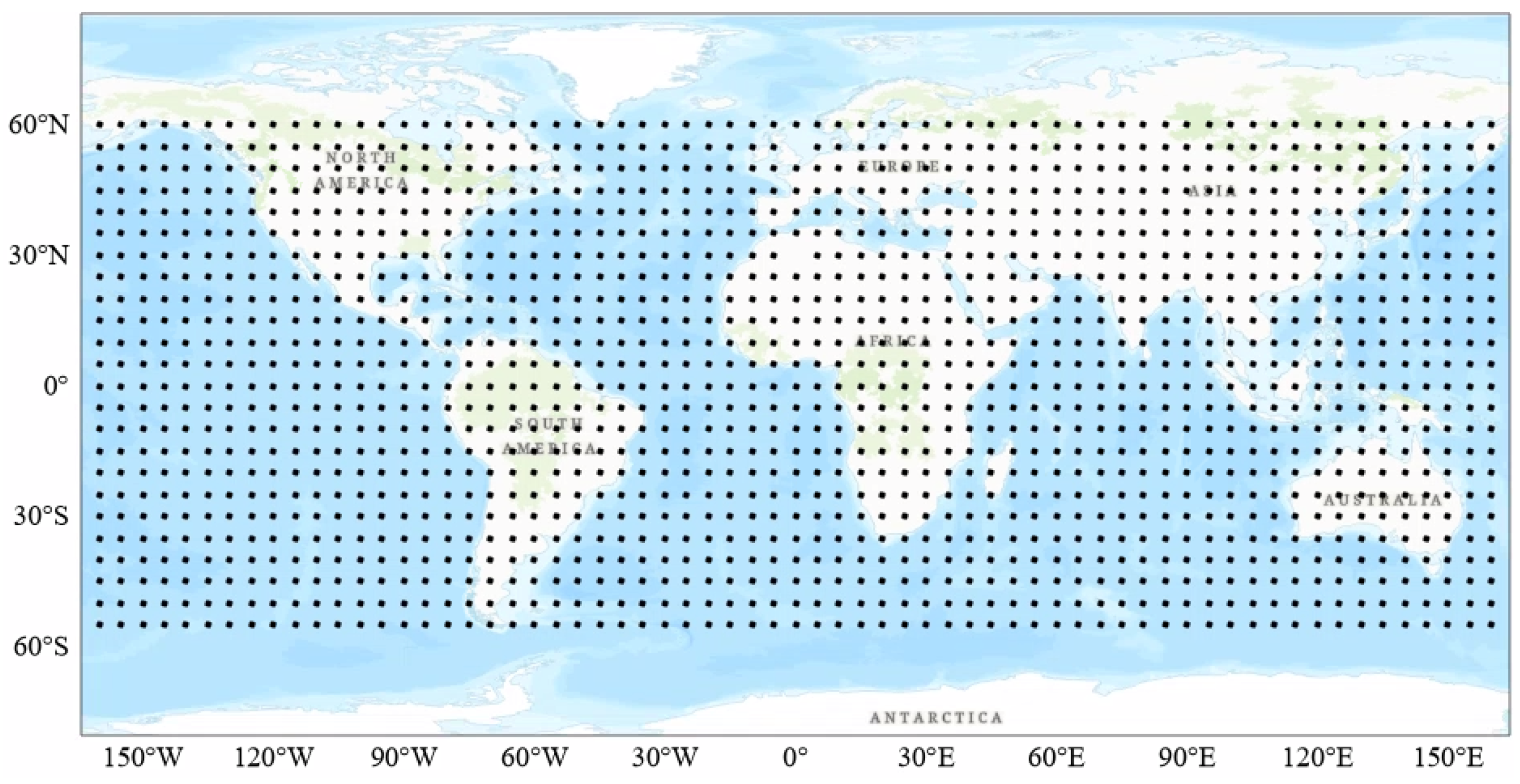
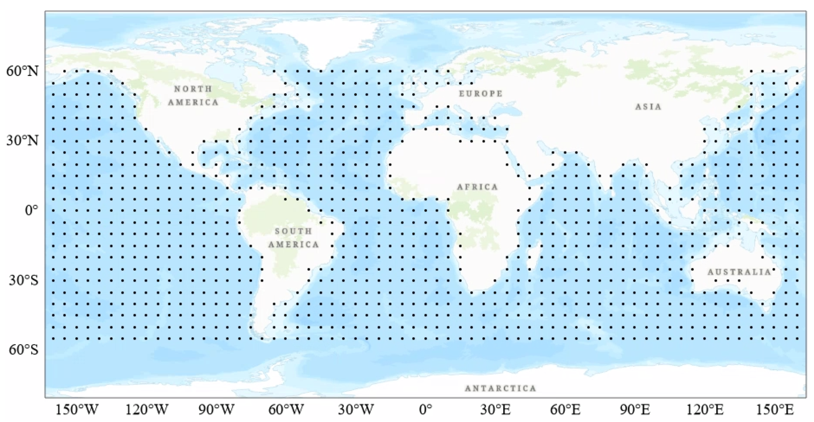
Linear models, such as least regression [13] and support vector machine [14,15], and non-linear models, such as decision trees [16] and random forest [17], are used for forecasting ENSO events. For example, in [13], the upper oceanic heat content and the thermocline depth at 20 °C isotherm are the variables used for forecasting. Ensemble learning is applied in both dynamical methods and statistical methods [17]. The three models used in the ensemble classifier are the artificial neural network, random forest, and nearest neighbor. The ensemble classifier uses the voting scheme to generate the final prediction. It correctly predicted 12 out of 13 central Pacific El Nino, 20 out of 20 eastern Pacific El Nino, 19 out of 26 La Nina, and 63 out of 64 neutral events. In a recent review [18], the application of machine learning algorithms and their role in improving the prediction skill of ENSO are discussed.

Recent studies applied artificial neural networks [19,20,21] convolutional neural networks (CNNs) [22,23,24], and recurrent neural networks [25,26,27] to ENSO forecasting. For example, in [22], CNN outperformed state-of-the-art dynamical models and achieved a CC of 0.5 for forecasting ONI for lead times of up to 17 months. Furthermore, the enhanced version of CNN, called all season-CNN (A-CNN), proposed in [23] improves the CC from 0.3 to 0.4 for a lead time of 23 months. A variant of CNN, such as the dense convolutional long short-term memory (DC-LSTM), is used in [28] for forecasting ENSO events. A dense convolutional layer and a transposed convolutional layer are used to extract the spatial features from the input, and multi-layer casual L-shaped LSTM is used to capture the temporal dynamics of SST anomalies. In addition to SST, T300 (vertically averaged oceanic temperature above 300 m), zonal wind, and meridional wind are used as predictors. Their results conclude that additional predictors showed no correlation with ENSO events. Although the performance of DC-LSTM is superior to that of CNN [22], the number of trainable parameters is relatively higher. Other variants, such as deformable CNN [29] and residual CNN [30], are also applied to forecast ENSO events.

Graph Neural Networks (GNNs) are the generalized version of CNNs that can handle non-Euclidean/non-uniform data. GNNs work well for spatial data as they can model the relationships between variables as graph edges. They are widely used in applications such as intelligent transportation, earthquake prediction, recommendation systems, and social media data-mining. However, it is surprising that GNNs are rarely applied in climate science and weather forecasting. Therefore, this study applies a graph-based approach, mainly AGCRNN, to forecast ONI for up to 18 months’ lead time. The main difference between our work and the other graph-based ENSO prediction [27] is that we learn the graph structure from the dataset during training, rather than learning a predefined graph structure that can be incomplete and inaccurate. Then, we modify feed-forward connections in the gated recurrent unit (GRU) with graph convolutions to capture the features’ spatial structure and temporal relationships with ONI.

3. Data Description

This study uses historical simulation and reanalysis datasets to forecast ONI, which is a three-month average of SST anomalies over the east–central equatorial Pacific region ranging from 5° N–5° S to 120° W–170° W. The historical simulation data were collected from 21 selected Coupled Model Intercomparison Project 5 (CMIP5) models. A single ensemble member from each CMIP5 model was chosen for 1860–2001. The reanalysis datasets were collected from Simple Ocean Data Assimilation (SODA) and Global Ocean Data Assimilation System (GODAS) for 1871–1973 and 1984–2017, respectively.

The study region contained both ocean and land data points (1728) collected across 0–360° E and 55° S–60° N with a 5° × 5° resolution, as shown in Figure 1. However, since SST and upper oceanic heat content are defined only for the ocean, we excluded land data points from our analysis, which resulted in 1345 data points, as shown in Figure 2. The features used in the study were three months’ SST and upper oceanic heat content anomalies measured at each point, and output was the ONI for a lead time of up to 18 months.

4. Methodology

Data standardization is a common process to standardize features in ML. Since both features (SST and upper oceanic heat content) have different ranges, we standardize them using the below equation, where x denotes a feature and $x_i$ denotes the value of that feature at a single data point.

$$\widehat{x_i}=\frac{x_i-mean\left(x\right)}{standarddeviation\left(x\right)}$$

(1)

4.1. Problem Statement

Consider a time series $X=\{X_{:,1},\dots ,X_{:,t},\dots \}$, where $X_{:,t}={\{x_{1,t},x_{2,t},\dots x_{N,t}\}}^T\in R^{\mathrm{N}\times 1}$ represents the observations recorded at N data points for time step t. Our goal is to predict the future values of the time series based on historical values. We formulated a spatial–temporal prediction problem to find a function F to forecast the next $\tau$ steps based on previous T historical values:

$$\{X_{:,t+1},X_{:,t+2},\dots ,X_{:,t+\tau }\}=F_{\theta }(X_{;,t},X_{:,t-1},\dots ,X_{t-T+1})$$

(2)

where $\theta$ denotes model parameters. The spatial correlations between different time series were formulated as a graph network. In an undirected graph network $G(V,E,A)$, $V_1,V_2,\dots V_N$ are the nodes of the graph, and E is the set of edges connecting the pairs of nodes. A node represents a data point based on latitude and longitude, and an edge represents the spatial connectivity between pair of data points. The adjacency matrix $A\in [0,1]$ representing the proximity between nodes is an $N\times N$ matrix where each entry $A_{ij}$ is the weighted representation of spatial similarity between nodes $V_i$ and $V_j$. If an edge exists between nodes $V_i$ and $V_j$, then $0<A_{ij}<1$; otherwise, $A_{ij}=0$. Therefore, the spatial–temporal prediction problem is modified by adding graph network G as follows:

$$\{X_{:,t+1},X_{:,t+2},\dots ,X_{:,t+\tau }\}=F_{\theta }(X_{;,t},X_{:,t-1},\dots ,X_{t-\tau +1};G)$$

(3)

4.2. Graph Learning Module (GLM)

Graph convolutional networks (GCNs) are applied in many domains, such as traffic prediction, urban anomaly prediction, recommendation systems, molecular biology, and social network analysis. A multi-layer GCN with layer-wise propagation is approximated using the first-order Chebyshev polynomial given by

$$H^{l+1}=\sigma \left({\tilde{D}}^{-\frac{1}{2}}\tilde{A}{\tilde{D}}^{-\frac{1}{2}}{H}^l{W}^l\right)$$

(4)

Here, $\tilde{A}=A+I_N$ is the adjacency matrix of the graph G with self-connections, $I_N$ is the identity matrix, D is the degree matrix and ${\tilde{D}}_{ii}={\sum }_j{\tilde{A}}_{ij}$. $W^l$ is a layer-specific trainable weight matrix. $\sigma (·)$ denotes an activation function, such as the $ReLU(·)=max(0,·)$. $H^l\in R^{N\times D}$ is the output of the $l^{th}$ layer and $H\left(0\right)=X$. More details of the first-order approximation are given in [31]. Most GCNs for prediction tasks rely on a predefined graph structure/adjacency matrix (A) computed using node distances or similarities to perform graph convolutions. Nevertheless, this predefined structure might not encompass all spatial dependencies, which can introduce bias into the model.

In this study, we used a graph learning module (GLM) to automatically infer the hidden dependencies from the data. First, the AGLM randomly initializes a learnable node-embedding matrix ($E_A\in R^{N\times d_e}$) for all nodes, where each row of $E_A$ represents the embedding of a node and $d_e$ represents the dimension of the node-embedding. Then, we can infer the spatial dependencies between pairs of nodes by multiplying $E_A$ and $E_A^T$. To reduce the computational cost, we directly generated the Laplacian Matrix ${\tilde{D}}^{-\frac{1}{2}}\tilde{A}{\tilde{D}}^{-\frac{1}{2}}$ using the following equation, where the SoftMax function normalizes the adaptive matrix.

$${\tilde{D}}^{-\frac{1}{2}}\tilde{A}{\tilde{D}}^{-\frac{1}{2}}=SoftMax\left(ReLU(E_A.E_A^T)\right)$$

(5)

During training, $E_A$ was updated automatically to learn the hidden dependencies between data points and generate the adaptive matrix for graph convolutions. Finally, by incorporating GLM into GCN, we obtained an adaptive graph convolution network (AGCN), given by the below equation:

$$H^{l+1}=SoftMax\left(ReLU(E_A.E_A^T)\right)H^l{W}^l$$

(6)

4.3. AGCRNN

The local and global spatial patterns are captured hierarchically using AGCN layers. However, to capture the temporal relationships, we proposed the use of AGCRNN by replacing fully connected Gated Recurrent Unit (GRU) layers with AGCN. The equations for AGCRNN are given by

$$\tilde{A}=SoftMax\left(ReLU\left(E{E}^T\right)\right)$$

(7)

$$z_t=\sigma (\tilde{A}[X_{:,t},h_{t-1}]W_z+b_z)$$

(8)

$$r_t=\sigma (\tilde{A}[X_{:,t},h_{t-1}]W_r+b_r)$$

(9)

$${\widehat{h}}_t=tanh(\tilde{A}[X_{:,t},r\odot h_{t-1}]W_{\widehat{h}}+b_{\widehat{h}})$$

(10)

$$h_t=z\odot h_{t-1}+(1-z)\odot {\widehat{h}}_t$$

(11)

where $[·]$ represents the concatenate operation, $X_{:,t}$$h_t$ are input and output at time step t, ⊙ represents element wise multiplication, and z and r represent the reset and update gate, respectively. The trainable parameters of AGCRNN are embedding matrix E, weights $W_Z,W_r,W_{\widehat{h}}$, and bias $b_Z,b_r,b_{\widehat{h}}$. All parameters are trained using the backpropagation algorithm.

4.4. Implementation Details

The AGCRNN architecture comprises an embedding layer, two AGCRNN layers, and a convolutional layer. The node-embedding layer takes the randomly initialized graph as input and assigns each node a low-dimensional embedding vector. Additionally, the node embeddings capture information about each node’s features and relationships with other nodes in the graph. The AGCRNN layers perform graph convolution on the node embeddings and dynamically adjust the graph structure during the convolution operation, enabling the network to learn the spatial structure of SST and upper-ocean heat content and their temporal relationships with ONI. Finally, a single convolutional filter with a kernel size of (nodes × hidden dimension of the previous layer) maps the output of the last AGCRNN layer to generate output. The AGCRNN’s network parameters are an embedding vector of size 10 and hidden layer of size 64. We optimized the AGCRNN using the Adam optimizer with a learning rate of 0.001 for a maximum of 100 epochs. Additionally, we implemented an early-stopping algorithm that halts training if the validation loss does not improve in the last 15 epochs. All parameters were selected through hyperparameter-tuning on the validation set.

For CMIP5 and SODA datasets, 60% of the data are used for training, 20% for validation, and 20% for testing. For the GODAS dataset, due to the relatively low number of samples (which might lead to overfitting), we followed the same procedure as detailed in [23]. Therefore, we used CMIP5, SODA, and GODAS for training, validation, and testing.

4.5. Model Evaluation

The performance of AGCRNN was compared with CNN [22] and eight dynamical models. Unfortunately, the results for the dynamical models are only available from 1984 to 2017. Therefore, for CMIP5 and SODA datasets, we compared the performance of AGCRNN with CNN alone, and for the GODAS dataset, we compared AGCRNN with CNN and dynamical models. Notably, only AGCRNN and CNN models were implemented in this study, while the results of the dynamical models are borrowed from [22].

We deployed two widely used regression metrics—correlation coefficient ($CC$) and coefficient of determination ($R^2$)—to compare the performance of the predictive models. $CC$ measures the strength of the relationship between actual and predicted values, while $R^2$ provides the variation in the actual values explained by the predictions. $C{C}^2$ = $R^2$ only if the prediction model is a linear regression and the mean of the predicted values equals the mean of the actual values. The mathematical formulation of these metrics is given by the following equations, where $y_i$ and $p_i$ denote the values of observed and predicted output for data point i and $\overline{y}$ and $\overline{p}$ indicate the mean of the output variable y and predicted variable p, respectively.

$$R^2=1-\frac{{\sum }_i{(p_i-\overline{y})}^2}{{\sum }_i{(y_i-\overline{y})}^2}$$

(12)

$$CC=\frac{{\sum }_i(p_i-\overline{p})(y_i-\overline{y})}{{\sum }_i{(p_i-\overline{p})}^2{\sum }_i{(y_i-\overline{y})}^2}$$

(13)

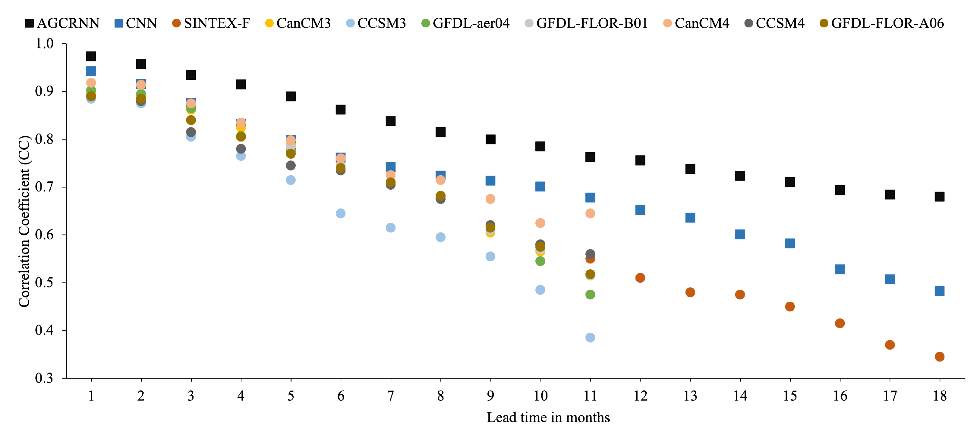
5. Results and Discussion

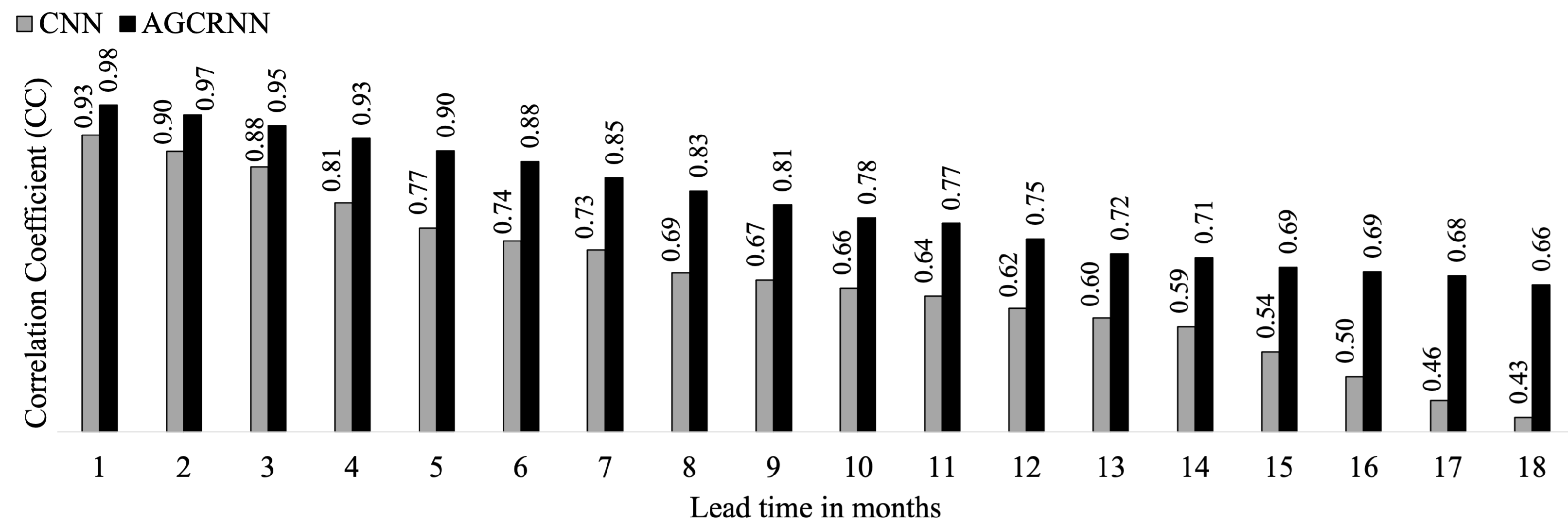
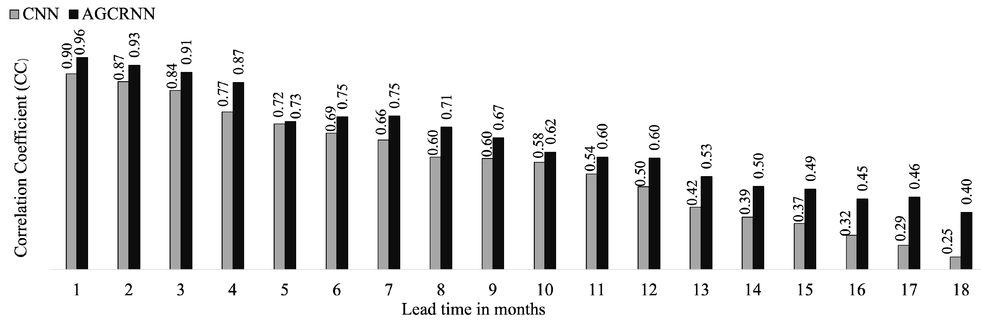
5.1. CMIP5 Dataset

In Figure 3, we compare the performance of CNN and AGCRNN for forecasting ONI using the CMIP5 dataset. Our proposed model outperforms CNN for all lead times, with a $CC$ of greater than 0.9 for up to five months compared to CNN’s performance of up to only two months. The rapid decrease in CNN’s performance after five months is due to its poor handling of irregular data, such as the missing land points in our dataset, which CNN fills with an average value. This approach can lead to a significant loss of information and bias in the model. In contrast, our proposed model is specifically designed to handle irregular data and uses graph-based operations to process the data effectively. Overall, these results highlight the advantages of our proposed AGCRNN model over CNN for forecasting ONI in the CMIP5 dataset.

In

Table 1. Coefficient of determination ($R^2$) of CNN and AGCRNN in forecasting ONI for CMIP5 dataset.

	Lead Time in Months
Model	1	2	3	4	5	6	7	8	9
CNN	0.86	0.81	0.79	0.70	0.65	0.61	0.55	0.53	0.51
AGCRNN	0.97	0.93	0.90	0.85	0.81	0.78	0.73	0.69	0.65
	10	11	12	13	14	15	16	17	18
CNN	0.46	0.42	0.41	0.37	0.33	0.32	0.30	0.25	0.21
AGCRNN	0.61	0.58	0.55	0.50	0.49	0.48	0.47	0.45	0.42

, we also compare the $R^2$ values of our model with CNN. Once again, our AGCRNN model outperforms CNN for all lead times, maintaining an $R^2$ value of 0.5 for up to 13 months’ lead time.

5.2. SODA Dataset

Figure 4 compares the performance of AGCRNN and CNN for forecasting ONI using the SODA dataset. Our proposed model outperforms CNN for all lead times. However, the $CC$ of both models on the SODA dataset is poorer than that of the CMIP5 dataset. This can be attributed to the smaller sample size of the SODA dataset, making models more susceptible to overfitting.

To further evaluate both models, we compare their $R^2$ values in

Table 2. Coefficient of determination ($R^2$) of CNN and AGCRNN in forecasting ONI for SODA dataset.

	Lead Time in Months
Model	1	2	3	4	5	6	7	8	9
CNN	0.72	0.64	0.60	0.55	0.47	0.42	0.41	0.45	0.42
AGCRNN	0.81	0.67	0.65	0.67	0.51	0.55	0.48	0.46	0.43
	10	11	12	13	14	15	16	17	18
CNN	0.36	0.34	0.28	0.18	0.18	0.17	0.15	0.16	0.09
AGCRNN	0.38	0.36	0.32	0.19	0.20	0.19	0.18	0.19	0.12

. Both models perform similarly in terms of $R^2$, indicating that a complex network structure does not improve the model performance for smaller datasets. Based on the results from both datasets, we conclude that the performance of AGCRNN improves for larger datasets. In other words, the ACGRNN’s performance is proportional to the sample size, as is the case for most deep-learning models.

5.3. GODAS Dataset

Figure 5 shows the $CC$ of statistical models (AGCRNN and CCN) and dynamical models (all other models) when forecasting ONI for various lead times using the GODAS dataset from 1984 to 2017. Among all models, AGCRNN exhibits the highest forecast skill for all lead times, surpassing both CNN and all other state-of-the-art dynamical models. CNN is the second-best performer, followed by SINTEX-F. AGCRNN achieves a $CC$ of 0.68 for an 18-month lead time, while CNN and SINTEX-F, the leading statistical and dynamical models, achieve 0.48 and 0.345, respectively. Consequently, we can conclude that AGCRNN can provide accurate ONI forecasts for up to 18 months of lead time. This superior performance of AGCRNN can be attributed to its proper representation of input features and adaptive graph structure, which capture the spatial structure of features and their temporal relationships with ONI.

Table 3. Coefficient of determination ($R^2$) of CNN and AGCRNN in forecasting ONI for GODAS dataset.

	Lead Time in Months
Model	1	2	3	4	5	6	7	8	9
CNN	0.92	0.89	0.83	0.76	0.71	0.67	0.63	0.59	0.55
AGCRNN	0.94	0.90	0.86	0.82	0.78	0.73	0.69	0.66	0.63
	10	11	12	13	14	15	16	17	18
CNN	0.52	0.48	0.46	0.43	0.38	0.36	0.35	0.31	0.28
AGCRNN	0.61	0.58	0.57	0.54	0.52	0.50	0.47	0.46	0.45

compares the $R^2$ values of statistical models since only $CC$ values are available for dynamical models. The $R^2$ values of AGCRNN are close to those of CNN for lead times up to 11 months. However, a substantial difference in $R^2$ values for higher lead times indicates that AGCRNN outperforms CNN in ONI forecasting.

6. Conclusions and Future Directions

This study uses an adaptive graph convolutional recurrent neural network (AGCRNN), a graph-based approach for forecasting ONI for up to 18 months’ lead time. Experiments on reanalysis and simulation datasets demonstrate that AGCRNN outperforms CNN [18] and eight dynamical models for all lead times. Specifically, for the 1984–2017 evaluation period, AGCRNN achieves a $CC$ of 0.68 for an 18-month lead time, while CNN and SINTEX-F, the leading statistical and dynamical models, achieve 0.48 and 0.345, respectively.

Our future work involves including other variables, such as southern oscillation index, warm water volume, and thermocline depth, as features, along with SST and upper ocean heat content. We also plan to explore better GCN architectures to understand the spatial structure of these features and their temporal relationships with ENSO.

References

1. Hardiman, S.C.; Dunstone, N.J.; Scaife, A.A.; Smith, D.M.; Ineson, S.; Lim, J.; Fereday, D. The impact of strong El Niño and La Niña events on the North Atlantic. Geophys. Res. Lett. 2019, 46, 2874–2883. [Google Scholar] [CrossRef]
2. Bjerknes, J. Atmospheric teleconnections from the equatorial Pacific. Mon. Weather. Rev. 1969, 97, 163–172. [Google Scholar] [CrossRef]
3. Cai, W.; Van Rensch, P.; Cowan, T.; Sullivan, A. Asymmetry in ENSO teleconnection with regional rainfall, its multidecadal variability, and impact. J. Clim. 2010, 23, 4944–4955. [Google Scholar] [CrossRef]
4. Yu, J.Y.; Fang, S.W. The distinct contributions of the seasonal footprinting and charged-discharged mechanisms to ENSO complexity. Geophys. Res. Lett. 2018, 45, 6611–6618. [Google Scholar] [CrossRef]
5. McPhaden, M.J.; Zhang, X. Asymmetry in zonal phase propagation of ENSO sea surface temperature anomalies. Geophys. Res. Lett. 2009, 36. [Google Scholar] [CrossRef] [Green Version]
6. Cole, J.E.; Overpeck, J.T.; Cook, E.R. Multiyear La Niña events and persistent drought in the contiguous United States. Geophys. Res. Lett. 2003, 29, 25-1–25-4. [Google Scholar] [CrossRef]
7. Hashemi, M.; Karimi, H. Weighted machine learning. Stat. Optim. Inf. Comput. 2018, 6, 497–525. [Google Scholar] [CrossRef]
8. Hashemi, M.; Karimi, H.A. Weighted machine learning for spatial-temporal data. IEEE J. Sel. Top. Appl. Earth Obs. Remote. Sens. 2020, 13, 3066–3082. [Google Scholar] [CrossRef]
9. Hashemi, M.; Alesheikh, A.A.; Zolfaghari, M.R. A spatio-temporal model for probabilistic seismic hazard zonation of Tehran. Comput. Geosci. 2013, 58, 8–18. [Google Scholar] [CrossRef]
10. Hashemi, M.; Alesheikh, A.A.; Zolfaghari, M.R. A GIS-based time-dependent seismic source modeling of Northern Iran. Earthq. Eng. Eng. Vib. 2017, 16, 33–45. [Google Scholar] [CrossRef]
11. Zhang, S.; Wang, H.; Jiang, H.; Ma, W. Evaluation of ENSO prediction skill changes since 2000 based on multimodel hindcasts. Atmosphere 2021, 12, 365. [Google Scholar] [CrossRef]
12. Saha, S.; Moorthi, S.; Wu, X.; Wang, J.; Nadiga, S.; Tripp, P.; Behringer, D.; Hou, Y.T.; Chuang, H.Y.; Iredell, M.; et al. The NCEP climate forecast system version 2. J. Clim. 2014, 27, 2185–2208. [Google Scholar] [CrossRef]
13. Lima, C.H.; Lall, U.; Jebara, T.; Barnston, A.G. Machine learning methods for ENSO analysis and prediction. In Machine Learning and Data Mining Approaches to Climate Science: Proceedings of the 4th International Workshop on Climate Informatics, Boulder, CO, USA, 25–26 September 2014; Springer: Cham, Switzerland, 2015; pp. 13–21. [Google Scholar]
14. Pal, M.; Maity, R.; Ratnam, J.V.; Nonaka, M.; Behera, S.K. Long-lead prediction of ENSO modoki index using machine learning algorithms. Sci. Rep. 2020, 10, 365. [Google Scholar] [CrossRef] [Green Version]
15. Aguilar-Martinez, S.; Hsieh, W.W. Forecasts of tropical Pacific sea surface temperatures by neural networks and support vector regression. Int. J. Oceanogr. 2009, 2009, 167239. [Google Scholar] [CrossRef] [Green Version]
16. Silva, K.A.; de Souza Rolim, G.; de Oliveira Aparecido, L.E. Forecasting El Niño and La Niña events using decision tree classifier. Theor. Appl. Climatol. 2022, 148, 1279–1288. [Google Scholar] [CrossRef]
17. Maher, N.; Tabarin, T.P.; Milinski, S. Combining machine learning and SMILEs to classify, better understand, and project changes in ENSO events. Earth Syst. Dyn. 2022, 13, 1289–1304. [Google Scholar] [CrossRef]
18. Dijkstra, H.A.; Petersik, P.; Hernández-García, E.; López, C. The application of machine learning techniques to improve El Niño prediction skill. Front. Phys. 2019, 7, 153. [Google Scholar] [CrossRef] [Green Version]
19. Baawain, M.S.; Nour, M.H.; El-Din, A.G.; El-Din, M.G. El Niño southern-oscillation prediction using southern oscillation index and Niño3 as onset indicators: Application of artificial neural networks. J. Environ. Eng. Sci. 2005, 4, 113–121. [Google Scholar] [CrossRef]
20. Tangang, F.T.; Hsieh, W.W.; Tang, B. Forecasting regional sea surface temperatures in the tropical Pacific by neural network models, with wind stress and sea level pressure as predictors. J. Geophys. Res. Ocean. 1998, 103, 7511–7522. [Google Scholar] [CrossRef]
21. Nooteboom, P.D.; Feng, Q.Y.; López, C.; Hernández-García, E.; Dijkstra, H.A. Using network theory and machine learning to predict El Niño. Earth Syst. Dyn. 2018, 9, 969–983. [Google Scholar] [CrossRef] [Green Version]
22. Ham, Y.G.; Kim, J.H.; Luo, J.J. Deep learning for multi-year ENSO forecasts. Nature 2019, 573, 568–572. [Google Scholar] [CrossRef] [PubMed]
23. Ham, Y.G.; Kim, J.H.; Kim, E.S.; On, K.W. Unified deep learning model for El Niño/Southern Oscillation forecasts by incorporating seasonality in climate data. Sci. Bull. 2021, 66, 1358–1366. [Google Scholar] [CrossRef] [PubMed]
24. Hashemi, M. Forecasting El Nino and La Nina Using Spatially and Temporally Structured Predictors and A Convolutional Neural Network. IEEE J. Sel. Top. Appl. Earth Obs. Remote. Sens. 2021, 14, 3438–3446. [Google Scholar] [CrossRef]
25. Broni-Bedaiko, C.; Katsriku, F.A.; Unemi, T.; Atsumi, M.; Abdulai, J.D.; Shinomiya, N.; Owusu, E. El Niño-Southern Oscillation forecasting using complex networks analysis of LSTM neural networks. Artif. Life Robot. 2019, 24, 445–451. [Google Scholar] [CrossRef]
26. Jonnalagadda, J.; Hashemi, M. Spatial-Temporal Forecast of the probability distribution of Oceanic Niño Index for various lead times. In Proceedings of the 33rd International Conference on Software Engineering and Knowledge Engineering, Virtual, 1–10 July 2021; p. 309. [Google Scholar]
27. Jonnalagadda, J.; Hashemi, M. Feature Selection and Spatial-Temporal Forecast of Oceanic Nino Index Using Deep Learning. Int. J. Softw. Eng. Knowl. Eng. 2022, 32, 91–107. [Google Scholar] [CrossRef]
28. Geng, H.; Wang, T. Spatiotemporal model based on deep learning for ENSO forecasts. Atmosphere 2021, 12, 810. [Google Scholar] [CrossRef]
29. Nielsen, A.H.; Iosifidis, A.; Karstoft, H. Forecasting large-scale circulation regimes using deformable convolutional neural networks and global spatiotemporal climate data. Sci. Rep. 2022, 12, 8395. [Google Scholar] [CrossRef]
30. Hu, J.; Weng, B.; Huang, T.; Gao, J.; Ye, F.; You, L. Deep residual convolutional neural network combining dropout and transfer learning for ENSO forecasting. Geophys. Res. Lett. 2021, 48, e2021GL093531. [Google Scholar] [CrossRef]
31. Defferrard, M.; Bresson, X.; Vandergheynst, P. Convolutional Neural Networks on Graphs with Fast Localized Spectral Filtering. Adv. Neural Inf. Process. Syst. 2016, 29, 3844–3852. [Google Scholar]
Figure 1. Data points are separated by 5° across latitude and longitude.
Engproc 39 00005 g001
Figure 2. Data points are separated by 5° across latitude and longitude after excluding points on land.
Engproc 39 00005 g002
Figure 3. Correlation Coefficient ( C C ) of CNN and AGCRNN in forecasting ONI for CMIP5 dataset.
Engproc 39 00005 g003
Figure 4. Correlation Coefficient ( C C ) of CNN and AGCRNN in forecasting ONI for SODA dataset.
Engproc 39 00005 g004
Figure 5. Correlation Coefficient ( C C ) of statistical models (CNN and AGCRNN) versus dynamical models for GODAS dataset.
Engproc 39 00005 g005