
Improving Predictive Accuracy in the Context of Dynamic Modelling of Non-Stationary Time Series with Outliers †


Abstract
1. Introduction
2. Methodologies
Outlier Detection and Treatment Procedures
- 1
- Linear interpolation (LI)
- Outlier detection: Observations are considered outliers if they are less than or greater than , where and denote the first and third quartiles, respectively, and (interquartile range) is the difference between the third and first quartiles ( rule).
- Outlier treatment: Any outliers that are identified are replaced by LI using the neighbouring observations [13].
- 2
- Iterative method based on the robust Kalman filter (RKF)
- Outlier detection: Outlier detection is performed by applying the rule on the standardized residuals after fitting a state-space model to the data.
- Outlier treatment: An alternative to the state estimator , inspired by the work by [14] and subsequently by [15], is proposed. In this approach, the state prediction is replaced bywhere is an identified outlier that is replaced by . This proposal considers the robust version of the Kalman filter only at moments at which outliers are detected, as opposed to the original work, in which it is applied at all moments. In the end, the model is iteratively fitted j times to the corrected time series until , , or for some value j.
- 3
- Iterative method based on the Kalman filter for time series with missing values (naKF)
- Outlier detection: Outlier detection is performed by applying the rule to the standardized residuals after fitting a state-space model to the data.
- Outlier treatment: Outlier observations are assumed to be missing values and the state estimator and its mean square error are replaced by and , respectively. The missing observations are replaced by and the state-space model is fitted j times to the corrected time series until , , or for some value j.
- ;
3. Results
3.1. Simulation Results
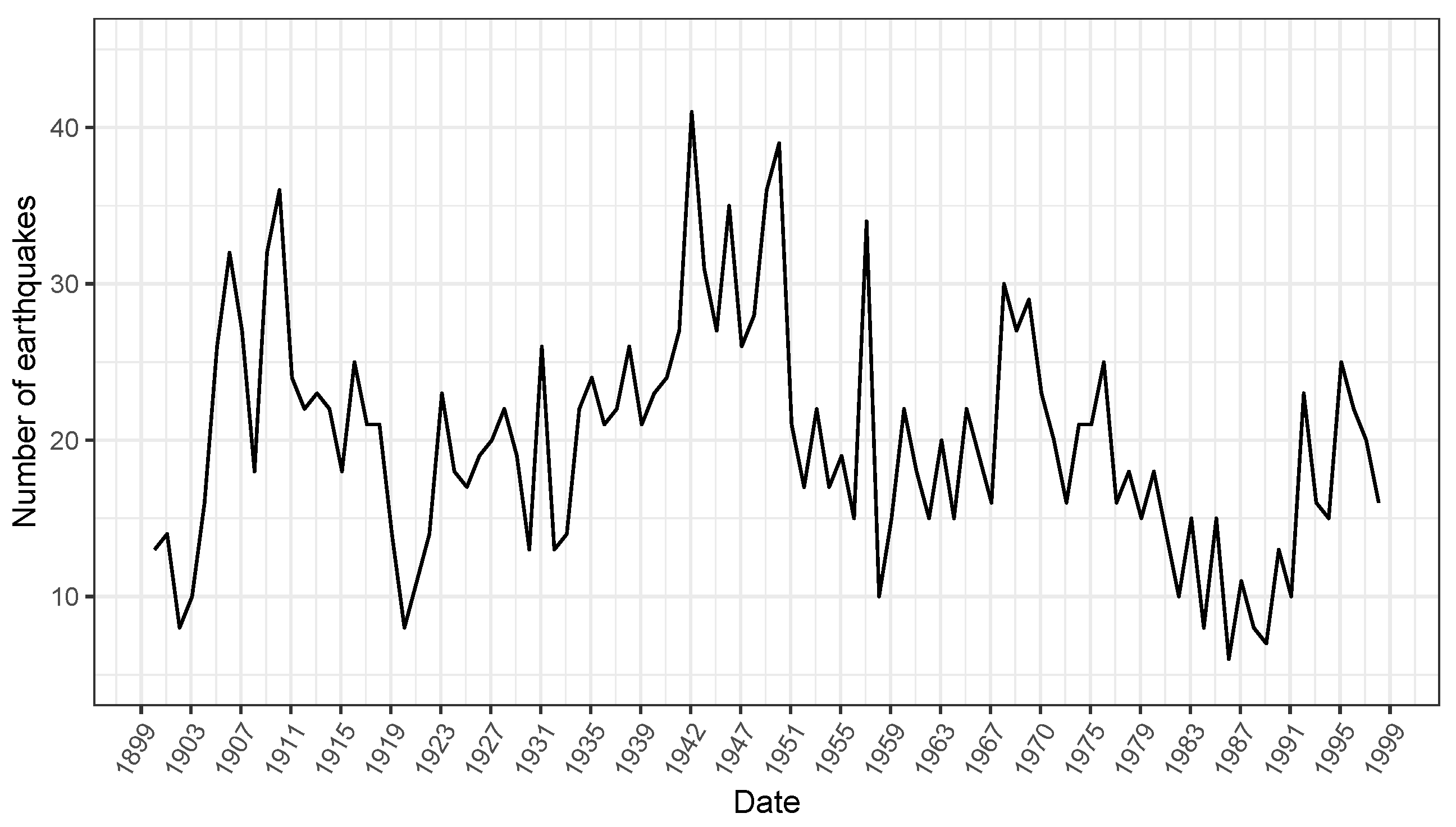
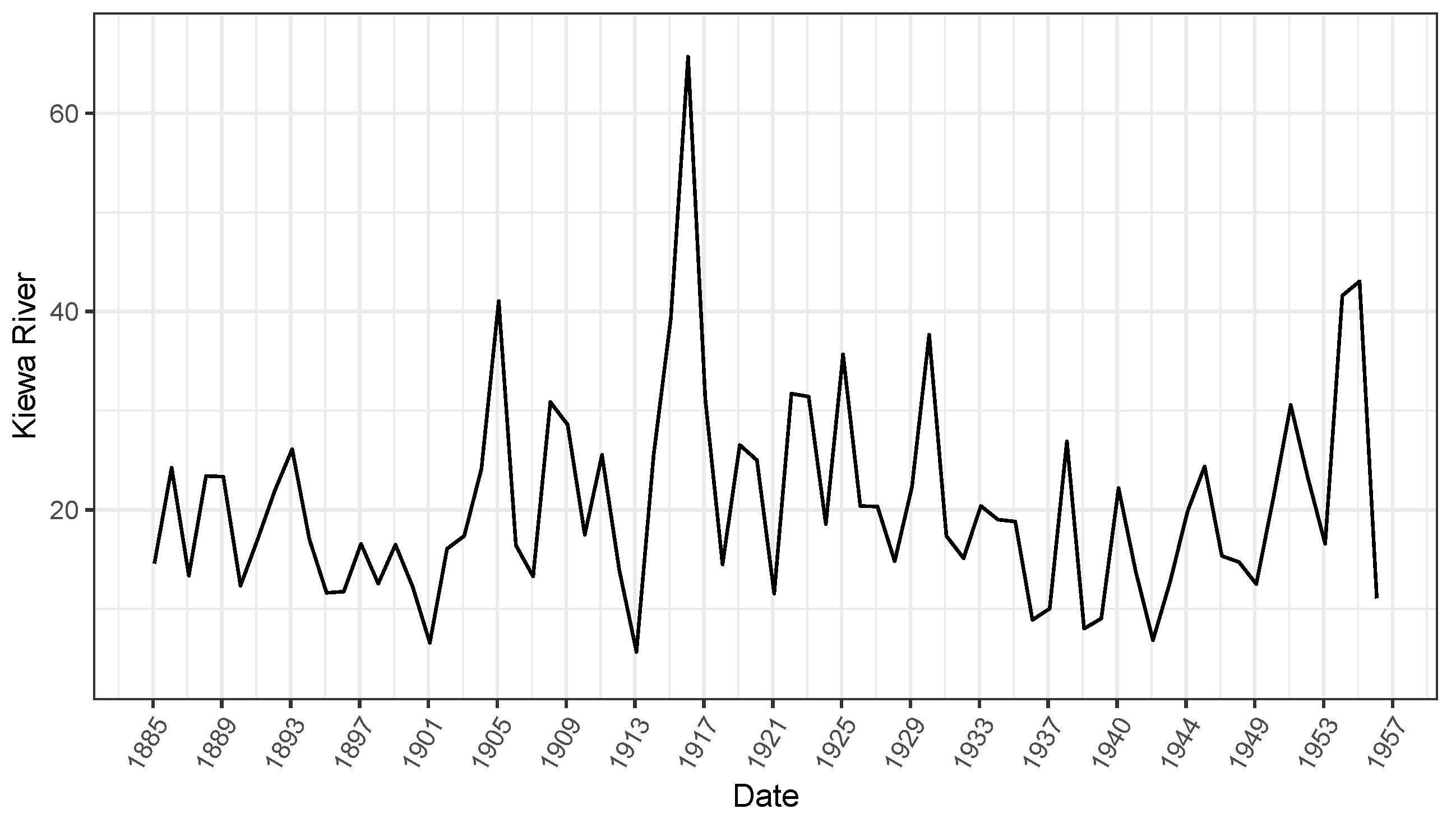
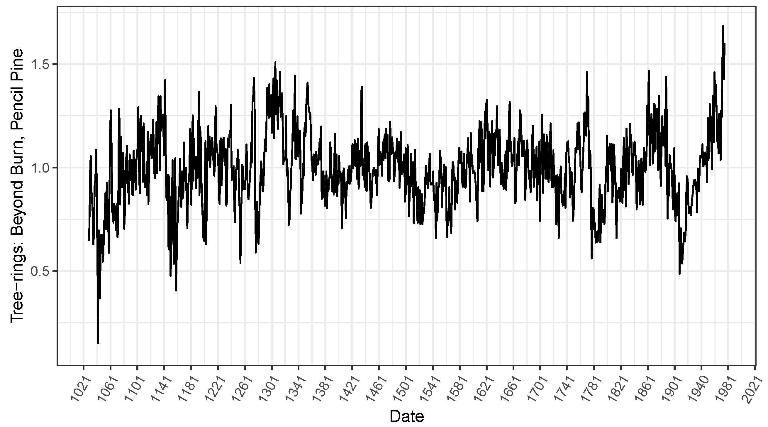
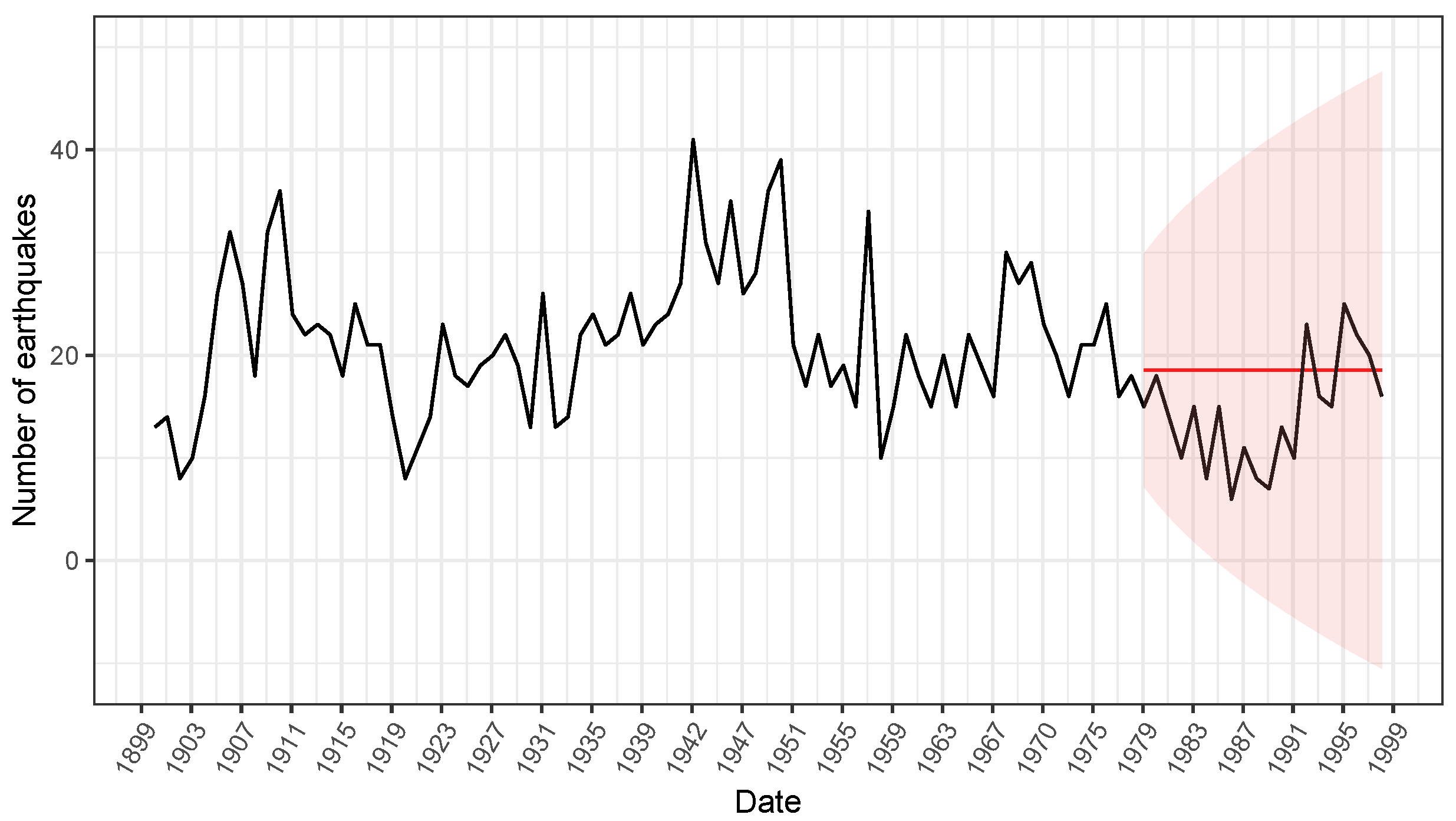
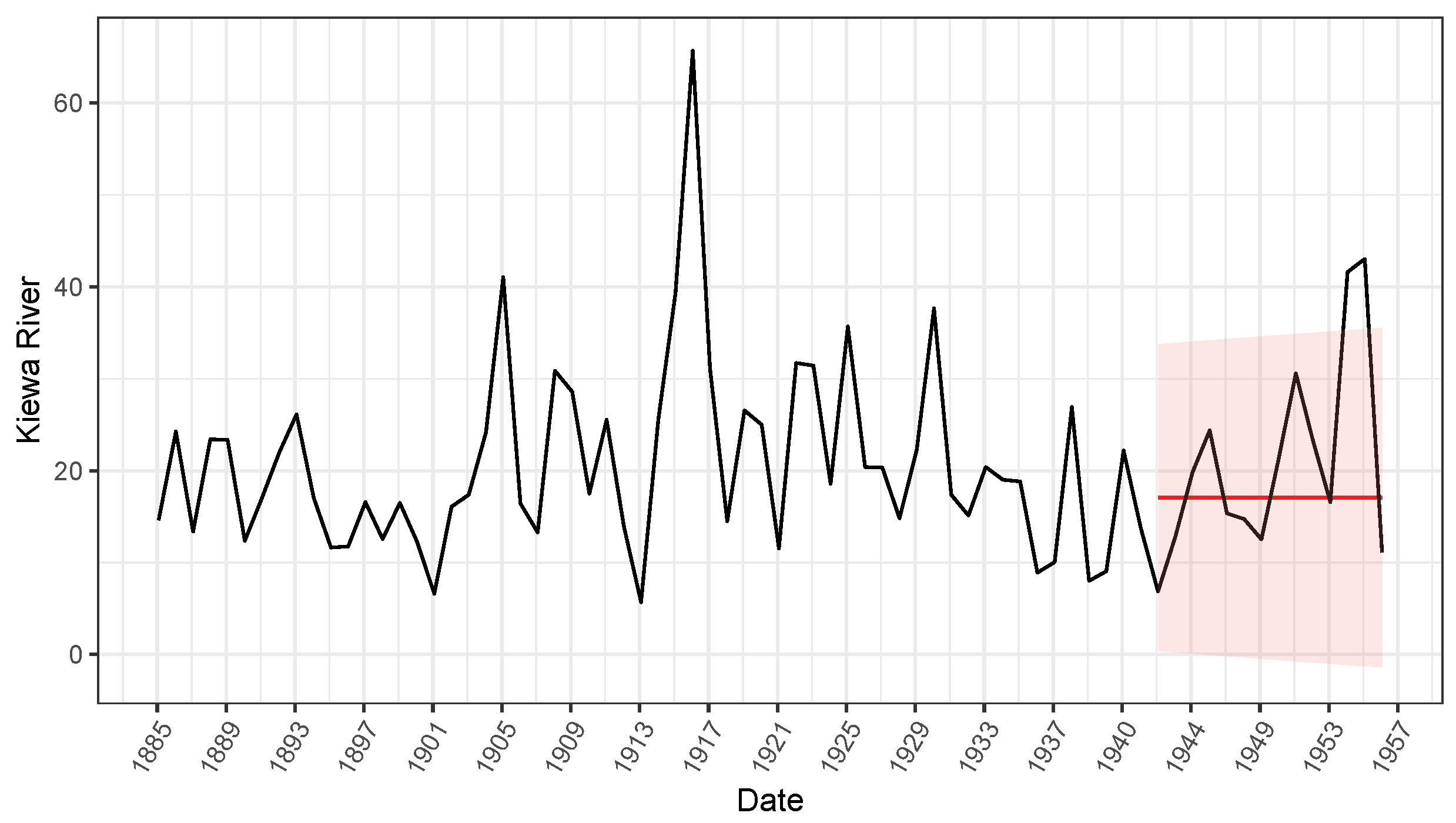
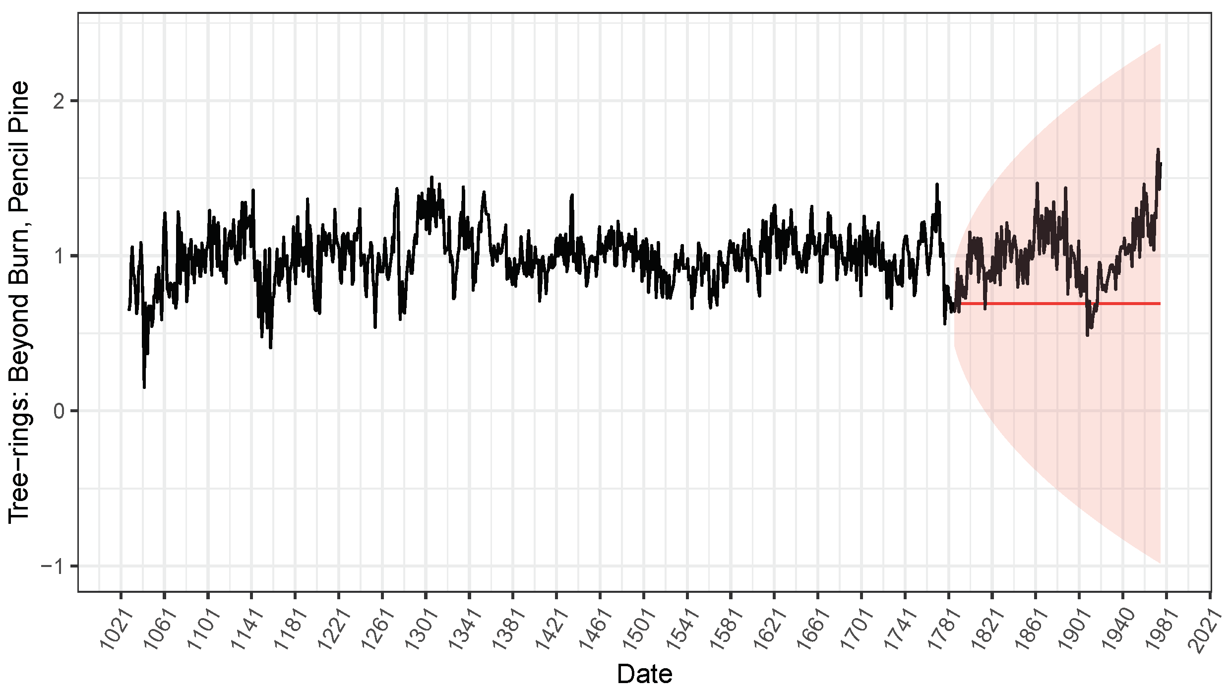
3.2. Illustrative Examples
4. Discussion
Author Contributions
Funding
Institutional Review Board Statement
Informed Consent Statement
Data Availability Statement
Acknowledgments
Conflicts of Interest
References
- Triantafyllopoulos, K. The State Space Model in Finance. In Bayesian Inference of State Space Models; Springer Texts in Statistics; Springer: Cham, Switzerland, 2021. [Google Scholar] [CrossRef]
- Auger-Methe, M.; Newman, K.; Cole, D.; Empacher, F.; Gryba, R.; King, A.A.; Leos-Barajas, V.; Flemming, J.M.; Nielsen, A.; Petris, G.; et al. A guide to state–space modeling of ecological time series. Ecol. Monogr. 2021, 91, 1–38. [Google Scholar] [CrossRef]
- Wu, H.; Matteson, D.; Wells, M. Interpretable Latent Variables in Deep State Space Models. arXiv 2022, arXiv:2203.02057. [Google Scholar]
- Matsuura, K. Time Series Data Analysis with State Space Model. In Bayesian Statistical Modeling with Stan, R, and Python; Springer: Singapore, 2022. [Google Scholar] [CrossRef]
- Monteiro, M.; Costa, M. Change Point Detection by State Space Modeling of Long-Term Air Temperature Series in Europe. Stats 2023, 6, 7. [Google Scholar] [CrossRef]
- Pereira, F.C.; Gonçalves, A.M.; Costa, M. Short-term forecast improvement of maximum temperature by state-space model approach: The study case of the TO CHAIR project. Stoch. Environ. Res. Risk Assess. 2023, 37, 219–231. [Google Scholar] [CrossRef]
- Shumway, R.H.; Stoffer, D.S. Time Series Analysis and its Applications: With R Examples; Springer: New York, NY, USA, 2017. [Google Scholar]
- Kalman, R. A New Approach to Linear Filtering and Prediction Problems. ASME J. Basic Eng. 1960, 82, 35–45. [Google Scholar] [CrossRef]
- Harvey, A. Forecasting, Structural Time Series Models and the Kalman Filter; Cambridge University Press: Cambridge, UK, 1990. [Google Scholar] [CrossRef]
- Teunissen, P.J.G.; Khodab, A.; Psychas, D. A generalized Kalman filter with its precision in recursive form when the stochastic model is misspecified. J. Geod. 2021, 95, 108. [Google Scholar] [CrossRef]
- Huang, Y.; Zhang, Y.; Zhao, Y.; Shi, P.; Chambers, J.A. A Novel Outlier-Robust Kalman Filtering Framework Based on Statistical Similarity Measure. IEEE Trans. Autom. Control 2021, 66, 2677–2692. [Google Scholar] [CrossRef]
- Auger-Méthé, M.; Field, C.; Albertsen, C.M.; Derocher, A.E.; Lewis, M.A.; Jonsen, I.D.; Flemming, J.M. State-space models’ dirty little secrets: Even simple linear Gaussian models can have estimation problems. Sci. Rep. 2016, 6, 26677. [Google Scholar] [CrossRef] [PubMed]
- Hyndman, R.J.; Athanasopoulos, G. Forecasting: Principles and Practice, 2nd ed.; OTexts: Melbourne, Australia, 2018. [Google Scholar]
- Cipra, T.; Romera, R. Kalman filter with outliers and missing observations. Test 1997, 6, 379–395. [Google Scholar] [CrossRef]
- Crevits, R.; Croux, C. Robust estimation of linear state space models. Commun. Stat.- Simul. Comput. 2019, 48, 1694–1705. [Google Scholar] [CrossRef]
- Durbin, J.; Koopman, S.J. Time Series Analysis by State Space Methods, 2nd ed.; Oxford Statistical Science Series; Oxford University Press: Oxford, UK, 2013. [Google Scholar] [CrossRef]


| Parameters | RMSE | MAE | Outlier | Mean | Mean | ||||||
|---|---|---|---|---|---|---|---|---|---|---|---|
| Detection | Rate 1 | Rate 2 | |||||||||
| 0.10 | 0.05 | NC | 0.0416 | 0.0276 | 0.4271 | 0.0335 | 0.0217 | 0.3399 | - | - | |
| C | 0.0621 | 0.2614 | 0.5243 | 0.0475 | 0.2214 | 0.4033 | - | - | |||
| LI | 0.0584 | 0.1772 | 0.4910 | 0.0438 | 0.1286 | 0.3781 | Time series | 84% | 42% | ||
| RKF | 0.0665 | 0.0910 | 0.4910 | 0.0456 | 0.0718 | 0.3781 | Standardized | 74% | 88% | ||
| naKF | 0.0536 | 0.0556 | 0.4667 | 0.0393 | 0.0337 | 0.3607 | residuals | ||||
| 1.00 | 0.10 | NC | 0.3114 | 0.1453 | 1.0734 | 0.2488 | 0.1088 | 0.8539 | - | - | |
| C | 0.4638 | 0.6275 | 1.2216 | 0.3644 | 0.4951 | 0.9507 | - | - | |||
| LI | 0.4255 | 0.5723 | 1.2127 | 0.3432 | 0.4499 | 0.9421 | Time series | 45% | 8% | ||
| RKF | 0.4216 | 0.4347 | 1.2048 | 0.3384 | 0.3422 | 0.9387 | Standardized | 61% | 42% | ||
| naKF | 0.4285 | 0.3821 | 1.2210 | 0.3422 | 0.2706 | 0.9383 | residuals | ||||
| 0.10 | 1.00 | NC | 0.0840 | 0.2456 | 1.1675 | 0.0618 | 0.1977 | 0.9326 | - | - | |
| C | 14.5332 | 468.2479 | 1.4690 | 1.3638 | 77.8606 | 1.1298 | - | - | |||
| LI | 0.1025 | 0.3266 | 1.1653 | 0.0719 | 0.2373 | 0.9250 | Time series | 91% | 99% | ||
| RKF | 0.3768 | 0.5958 | 1.2860 | 0.1245 | 0.3587 | 0.9876 | Standardized | 78% | 98% | ||
| naKF | 0.4510 | 0.3155 | 1.2844 | 0.1582 | 0.2525 | 0.9620 | residuals | ||||
| 0.05 | 0.10 | NC | 0.0275 | 0.0329 | 0.4413 | 0.0212 | 0.0260 | 0.3517 | - | - | |
| C | 0.0564 | 0.4242 | 0.5416 | 0.0333 | 0.3516 | 0.4180 | - | - | |||
| LI | 0.0343 | 0.1501 | 0.4663 | 0.0237 | 0.0830 | 0.3652 | Time series | 91% | 83% | ||
| RKF | 0.0586 | 0.0710 | 0.4914 | 0.0327 | 0.0557 | 0.3798 | Standardized | 75% | 97% | ||
| naKF | 0.0476 | 0.0391 | 0.4714 | 0.0279 | 0.0294 | 0.3635 | residuals | ||||
| Parameters | RMSE | MAE | Outlier | Mean | Mean | ||||||
|---|---|---|---|---|---|---|---|---|---|---|---|
| Detection | Rate 1 | Rate 2 | |||||||||
| 0.10 | 0.05 | NC | 0.0138 | 0.0086 | 0.4315 | 0.0109 | 0.0068 | 0.3443 | - | - | |
| C | 0.0170 | 0.2228 | 0.5303 | 0.0137 | 0.2187 | 0.4115 | - | - | |||
| LI | 0.0184 | 0.2156 | 0.5561 | 0.0147 | 0.2112 | 0.4193 | Time series | 52% | 4% | ||
| RKF | 0.0189 | 0.0696 | 0.4913 | 0.0146 | 0.0684 | 0.3822 | Standardized | 77% | 91% | ||
| naKF | 0.0181 | 0.0133 | 0.4656 | 0.0137 | 0.0103 | 0.3613 | residuals | ||||
| 1.00 | 0.10 | NC | 0.1156 | 0.0524 | 1.0891 | 0.0934 | 0.0419 | 0.8685 | - | - | |
| C | 0.1376 | 0.4955 | 1.2374 | 0.1112 | 0.4775 | 0.9679 | - | - | |||
| LI | 0.1454 | 0.4962 | 1.3117 | 0.1165 | 0.4788 | 0.9915 | Time series | 19% | 1% | ||
| RKF | 0.1366 | 0.3261 | 1.2226 | 0.1102 | 0.3114 | 0.9550 | Standardized | 65% | 41% | ||
| naKF | 0.1643 | 0.2065 | 1.2561 | 0.1272 | 0.1803 | 0.9634 | residuals | ||||
| 0.10 | 1.00 | NC | 0.0235 | 0.0771 | 1.1685 | 0.0188 | 0.0610 | 0.9324 | - | - | |
| C | 0.0351 | 4.7013 | 1.4334 | 0.0275 | 4.6231 | 1.1320 | - | - | |||
| LI | 0.0341 | 2.0559 | 1.2754 | 0.0242 | 1.3978 | 1.0019 | Time series | 94% | 68% | ||
| RKF | 0.0299 | 0.2428 | 1.2191 | 0.0227 | 0.2255 | 0.9664 | Standardized | 89% | 100% | ||
| naKF | 0.0423 | 0.1168 | 1.1950 | 0.0254 | 0.0976 | 0.9436 | residuals | ||||
| 0.05 | 0.10 | NC | 0.0086 | 0.0100 | 0.4466 | 0.0068 | 0.0079 | 0.3561 | - | - | |
| C | 0.0125 | 0.4614 | 0.5647 | 0.0098 | 0.4517 | 0.4417 | - | - | |||
| LI | 0.0119 | 0.3605 | 0.5628 | 0.0094 | 0.3348 | 0.4290 | Time series | 81% | 23% | ||
| RKF | 0.0116 | 0.0722 | 0.4893 | 0.0088 | 0.0702 | 0.3854 | Standardized | 84% | 99% | ||
| naKF | 0.0104 | 0.0129 | 0.4617 | 0.0077 | 0.0106 | 0.3644 | residuals | ||||
| Estimate | (SE) | Estimate | (SE) | |||
|---|---|---|---|---|---|---|
| TS1 | Non-treated | 2.7103 | (0.6932) | 4.8341 | (0.5760) | −192.8515 |
| LI | 2.6438 | (0.6735) | 4.6330 | (0.5578) | −190.1958 | |
| RKF | 2.9174 | (0.6983) | 4.0890 | (0.5653) | −185.7237 | |
| naKF | 3.0671 | (0.7237) | 3.8387 | (0.5844) | −183.6041 | |
| TS2 | Non-treated | 1.6446 | (0.8822) | 9.3662 | (0.9774) | −170.7793 |
| LI | 1.2913 | (0.7006) | 7.8502 | (0.8092) | −161.2743 | |
| RKF | 1.1704 | (0.6859) | 7.7522 | (0.7959) | −160.3136 | |
| naKF | 1.0999 | (0.6905) | 7.7692 | (0.7967) | −158.2455 | |
| TS3 | Non-treated | 0.0623 | (0.0058) | 0.1054 | (0.0046) | 1096.8770 |
| LI | 0.0597 | (0.0057) | 0.0971 | (0.0045) | 1149.8800 | |
| RKF | 0.0614 | (0.0055) | 0.1000 | (0.0044) | 1129.9350 | |
| naKF | 0.0601 | (0.0055) | 0.1020 | (0.0044) | 1124.1500 | |
| Non-Treated | LI | RKF | naKF | ||||||
|---|---|---|---|---|---|---|---|---|---|
| RMSE | MAE | RMSE | MAE | RMSE | MAE | RMSE | MAE | ||
| TS1 | vs. | 7.0245 | 6.0496 | 7.0087 | 6.0353 | 6.8205 | 5.8609 | 6.7342 | 5.7788 |
| Percentage reduction | - | - | 0.22% | 4.14% | 2.90% | 3.12% | 4.13% | 4.48% | |
| TS2 | vs. | 11.4091 | 8.1459 | 11.3624 | 8.1456 | 11.2833 | 8.1455 | 11.2249 | 8.1455 |
| Percentage reduction | - | - | 0.41% | 0.004% | 1.10% | 0.01% | 1.61% | 0.01% | |
| TS3 | vs. | 0.3759 | 0.3231 | 0.3757 | 0.3229 | 0.3756 | 0.3228 | 0.3742 | 0.3213 |
| Percentage reduction | - | - | 0.05% | 0.06% | 0.08% | 0.09% | 0.45% | 0.56% | |
Disclaimer/Publisher’s Note: The statements, opinions and data contained in all publications are solely those of the individual author(s) and contributor(s) and not of MDPI and/or the editor(s). MDPI and/or the editor(s) disclaim responsibility for any injury to people or property resulting from any ideas, methods, instructions or products referred to in the content. |
© 2023 by the authors. Licensee MDPI, Basel, Switzerland. This article is an open access article distributed under the terms and conditions of the Creative Commons Attribution (CC BY) license (https://creativecommons.org/licenses/by/4.0/).
Share and Cite
Pereira, F.C.; Gonçalves, A.M.; Costa, M. Improving Predictive Accuracy in the Context of Dynamic Modelling of Non-Stationary Time Series with Outliers. Eng. Proc. 2023, 39, 36. https://doi.org/10.3390/engproc2023039036
Pereira FC, Gonçalves AM, Costa M. Improving Predictive Accuracy in the Context of Dynamic Modelling of Non-Stationary Time Series with Outliers. Engineering Proceedings. 2023; 39(1):36. https://doi.org/10.3390/engproc2023039036
Chicago/Turabian StylePereira, Fernanda Catarina, Arminda Manuela Gonçalves, and Marco Costa. 2023. "Improving Predictive Accuracy in the Context of Dynamic Modelling of Non-Stationary Time Series with Outliers" Engineering Proceedings 39, no. 1: 36. https://doi.org/10.3390/engproc2023039036
APA StylePereira, F. C., Gonçalves, A. M., & Costa, M. (2023). Improving Predictive Accuracy in the Context of Dynamic Modelling of Non-Stationary Time Series with Outliers. Engineering Proceedings, 39(1), 36. https://doi.org/10.3390/engproc2023039036