Abstract
Accurate precipitation forecasting is essential for emergency management, aviation, and marine agencies to prepare for potential weather impacts. However, traditional radar echo extrapolation has limitations in capturing sudden weather changes caused by convective systems. Deep learning models, an alternative to radar echo extrapolation, have shown promise in precipitation nowcasting. However, the quality of the forecasted radar images deteriorates as the forecast lead time increases due to mean absolute error (MAE, a.k.a L1) or mean squared error (MSE, a.k.a L2), which do not consider the perceptual quality of the image, such as the sharpness of the edges, texture, and contrast. To improve the quality of the forecasted radar images, we propose using the Structural Similarity (SSIM) metric as a regularization term for the Conditional Generative Adversarial Network (CGAN) objective function. Our experiments on satellite images over the region 83° W–76.5° W and 33° S–40° S in 2020 show that the CGAN model trained with both L1 and SSIM regularization outperforms CGAN models trained with only L1, L2, or SSIM regularizations alone. Moreover, the forecast accuracy of CGAN is compared with other state-of-the-art models, such as U-Net and Persistence. Persistence assumes that rainfall remains constant for the next few hours, resulting in higher forecast accuracies for shorter lead times (i.e., <2 h) measured by the critical success index (CSI), probability of detection (POD), and Heidtke skill score (HSS). In contrast, CGAN trained with L1 and SSIM regularization achieves higher CSI, POD, and HSS for lead times greater than 2 h and higher SSIM for all lead times.
1. Introduction
In recent years, rapid climate change and global warming have led to catastrophic weather events, such as heavy rainfall and flash floods in various parts of the world [1]. Heavy rains, followed by strong winds, can cause significant economic and social losses. “Precipitation nowcasting” refers to forecasting rainfall intensity in a region over a relatively short period (between 0 and 4 h). Precipitation nowcasting provides multiple sectors, including emergency management services, flood warning systems, and flight and marine operations, with warnings before heavy rainfalls. Additionally, short-term weather forecasts are critical for outdoor activities, such as construction, roadworks, sports, and community gatherings.
Deep Learning (DL) has revolutionized the field of computer vision due to its ability to capture semantic information from images and videos [2]. Despite the promising performance of current state-of-the-art models in predicting future radar echoes, the quality of the predictions generated by these models is poor, often referred to as blurry predictions in the literature [3,4]. For instance, using Mean Squared Error (MSE, a.k.a L2) or Mean Absolute Error (MAE, a.k.a L1) losses in image-to-image prediction problems produces low-quality images due to uniform distribution assumption, which is not valid for multi-modal data distribution. In addition, both L1 and L2 losses force the model to generate a mean prediction of all possible outcomes, thereby losing sharp details such as edges and color transitions between pixels.
The main contribution of this study is to improve the quality of forecasted images by introducing an image quality metric, Structural Similarity (SSIM), as a regularization term for the objective function of the Conditional Generative Adversarial Network (CGAN). The SSIM is a visual image quality metric that measures structural changes such as local structure, luminosity, and contrast between the ground truth and generated images. This study conducts several experiments to demonstrate the superiority of the SSIM regularization over other pixel-wise regularization approaches, such as L1 and L2, measured in terms of the critical success index (CSI), false alarm ratio (FAR), Heidtke Skill Score (HSS), probability of detection (POD), and SSIM.
The rest of the paper is organized as follows. Section 2 reviews the relevant literature on precipitation nowcasting. Section 3 describes the data and preprocessing, followed by the proposed methodology in Section 4. Finally, Section 5 discusses the experimental results, and Section 6 concludes the paper with a summary of findings and future directions.
2. Literature Review
Both theoretical [5,6] and practical [7,8,9,10,11] application of ML in forecasting and predicting spatial–temporal phenomena has been underscored in the literature. Random forest and decision tree performed better in rainfall forecasting for shorter lead times [12,13]. Prudden et al. [14] comprehensively reviewed existing methods in radar-based nowcasting. This study sheds light on the limitations of optical flow-based and persistence-based methods and the scope of ML methods in precipitation nowcasting.
DL models are widely used in precipitation nowcasting. U-Net is a convolutional neural network (CNN) commonly used for precipitation nowcasting [15]. A Small Attention U-Net (SmaAt-UNet) was developed by adding an attention module and depth-wise convolutions to the original U-Net architecture [16]. Although SmaAt-UNet performs the same as U-Net, the number of trainable parameters is reduced to one-quarter. RainNet, another member of the U-Net family, is inspired by SegNet and used in radar-based nowcasting [17]. The attention mechanism in deep learning has shown promising results in computer vision. Yan et al. [18] proposed multi-head attention in a dual-channel network to highlight the critical areas of precipitation. Results indicate that the addition of multi-head attention and residual connections to the CNN can precisely extract the local and global spatial features of the radar image.
Some studies have used ConvLSTM for precipitation nowcasting [19,20,21]. Shi et al. proposed two DL models, Trajectory Gated Recurrent Unit (TrajGRU) [22] and ConvLSTM [23], for precipitation nowcasting. TrajGRU overcomes the location invariance problem in ConvLSTM using fewer training parameters. Most recent studies have applied generative adversarial networks (GANs) [24] for weather forecasting [25]. For instance, Choi and Kim [26] trained Radar CGAN on radar images with a spatial resolution of 128 × 128 km and a temporal resolution of 10 min. They showed that Rad-CGAN outperforms U-Net and ConvLSTM in terms of CSI. Few studies use satellite images for precipitation nowcasting. Hayatbini et al. [27] used satellite images and applied CGANs to generate forecasts over the contiguous United States for up to four hours of lead times. Their model outperformed Precipitation Estimation from Remotely Sensed Information using Artificial Neural Networks for Cloud Classification System (PERSIAN-CSS) in terms of CSI, POD, FAR, MSE, bias, and correlation coefficient. Despite the use of advanced DL models, such as U-Net, and GANs in precipitation nowcasting, the predicted images often turn out to be blurry due to the L1 or L2 losses [3,4].
3. Data Description
The dataset used in this study was collected from the National Aeronautics and Space Administration’s (NASA’s) Integrated Multi-Satellite Retrievals for Global Precipitation Measurement (IMERG) algorithm [28], which provides precipitation estimates with a spatial resolution of 0.1° × 0.1° (10 km × 10 km) all over the globe. We used half-hourly final IMERG data from 1 January 2020–31 December 2020, positioned over the east coast of the United States (−83° W–76.5° W, 33° S–40° S) with a spatial resolution of 0.1° × 0.1° (10 km × 10 km) and precipitationCal as the variable of interest.
Our dataset is multidimensional, with latitude, longitude, and timestamp as dimensions. Our program reads through the dataset for each timestamp and constructs a two-dimensional matrix (also called a rain map) based on latitude and longitude. A rain map represents the snapshot of the precipitation collected over the study region. The rain maps have a dimension of 64 × 64, with each pixel representing average rainfall in the last 30 min over 10 km × 10 km. Most rain maps contain pixels with low or no rain, so we created two balanced datasets, Dataset-A and Dataset-B, by ensuring that each rain map has a minimum number of rainy pixels, following a similar approach to that shown in [24]. Dataset-A contains at least 50% of pixels with rain, while Dataset-B contains at least 20%. Both datasets have gaps in the timestamps because the rain maps that do not qualify for the threshold were dismissed. We handle the gaps in both datasets by creating an empty set and adding samples to it sequentially until the first gap is identified. We follow the same process through the end of the dataset, generating several small subsets. Finally, we treat each subset as a separate dataset and create input and output sequences. The input to the model is a sequence of four rain maps (past 2 h) stacked along the channel dimension, and the output from the model is a single rain map at a lead time of 30 min, 1 h, 2 h, or 4 h. Therefore, the input and output dimensions are (64 × 64 × 4) and (64 × 64 × 1), respectively.
Dataset-A and Dataset-B are balanced datasets containing 944 and 3736 samples, respectively. Although they have fewer samples than the original dataset (17,548), they are suitable for this study to predict rainfall. Therefore, we evaluate our proposed model on these two datasets. In the results section of this paper, we provide a detailed comparison of CGAN’s performance on both datasets.
4. Methodology
4.1. Problem Statement
The radar echo extrapolation task can be viewed as a sequence-to-sequence prediction problem as it considers the historical radar echo maps to forecast future radar echo maps. The radar echo map/rain map at any time t is a tensor of shape , where A and B represent a rain map’s height (rows) and width (columns). In this study, . The sequence of tensors from to T is obtained by collecting rain maps at fixed time intervals over T. Therefore, the spatial–temporal prediction problem can be obtained by finding a function F to forecast a rain map at l time steps ahead given the sequence of j rain maps, as shown below:
where denotes model parameters. In this study, the temporal interval between rain maps is 30 min. The size of the rain map is 64 × 64, the value of j is empirically chosen to be 4, and l is varied up to 8. For example, when j = 4 and l = 8, the past two hours of rain maps are used to forecast a rain map after four hours.
4.2. Conditional Generative Adversarial Network (CGAN)
This study applies CGANs for precipitation nowcasting. GANs are generative models that learn a mapping from a random noise vector z to output image y, G: z → y [29]. In contrast, CGANs learn a conditional generative model, i.e., instead, CGANs learn a mapping from both an auxiliary information x and noise random vector z to output image y, G: {x, z} → y [30]. The following equation gives the objective function of CGAN:
where the generator (G) tries to minimize the objective against its opponent discriminator (D), whereas D tries to maximizes the objective against its adversary G, and the loss function of CGAN denoted as is given by
The use of pixel-wise loss functions such as L1 or L2 in the objective function of CGAN is common in precipitation nowcasting literature [25,26,27]. This allows the generator to produce images with pixel values close to the ground truth. However, a common limitation of L1 or L2 loss functions is blurriness in the forecasts. This is because L1 or L2 loss functions assume that noise is independent of the local image characteristics, whereas the sensitivity of the Human Visual System (HVS) depends on the structural changes such as local contrast, luminance, and structure. Other studies [4] support this argument, suggesting that L1 or L2 loss functions assume global similarity but do not capture local structures or intricate characteristics of the HVS, such as edges and color transitions between pixels.
4.3. CGAN with SSIM Regularization
To improve the quality of forecasted images, this study introduces the SSIM loss as a regularization to the objective function of CGAN, which is given by the below equation.
where is the SSIM of the kth kernel window of the output image (y) and generated image (), respectively, and M is the number of kernels. The penalty factor is set empirically. When is set to zero, CGAN is trained using only the adversarial loss. If is set to one, both the adversarial loss and SSIM loss are used in equal proportions during training. However, if is set to a much larger value, the training of CGAN is primarily optimized to minimize errors caused by the loss of structural information.
The Structural Similarity (SSIM) [31] is a perceptual metric that measures the quality of an image. Unlike other metrics, SSIM requires both a reference image and a processed image to calculate the similarity between the two. We use the following formula to compute the SSIM value for two equal sized windows i and j of reference and processed image. For simplicity, we use the notations i and j instead of and .
where the symbols , , , and represent the mean and standard deviation of pixel values within windows i and j, respectively. The symbol represents the covariance between the pixel values of windows i and j. The constants and are given by and , respectively, where and are default values of 0.01 and 0.03, and L is the dynamic range of pixels, which is .
Studies show that training deep learning models with a combined SSIM loss function and pixel-wise losses such as L1 or L2 loss can improve the quality of forecasts for image-to-image translation problems [32,33]. This is because L1 or L2 loss functions preserve colors and luminance (local structure), whereas the SSIM loss function preserves contrast. Therefore, we analyze the performance of CGAN by training the generator using different combinations of SSIM and L1 or L2 loss functions. Excluding random noise (z) from Equation (4), the generator can still learn a mapping from x to y, but it is highly sensitive to randomness because slight changes in x can significantly vary y. Our experimental results found that the noise vector z has no impact on generator training because the same results were produced with and without the noise vector. Therefore, we ignore the noise vector z from the generator and instead use dropout as noise in the layers of the generator during training and testing [30]. In pix2pix CGAN, U-Net is used for the generator and Patch-GAN is used for the discriminator. It is worth noting that we utilized the pix2pix version of CGAN [30], but with a slightly modified U-Net generator designed to fit the size of our input image (64 × 64). Adam is the optimizer used with a learning rate of 0.0002, and momentum parameters are 0.5 and 0.99. We determined the optimal hyperparameter values for epochs, batch size, and penalty factor () through hyperparameter tuning on the validation set. The resulting values are as follows: 100 epochs, a batch size of 16, and a penalty factor of 100. The patch size of the discriminator (a.k.a discriminator receptive field) is set to 1 × 1 (PixelGAN).
4.4. Baselines (U-Net and Persistence)
To compare the performance of CGAN, we utilized two state-of-the-art baselines: U-Net and Persistence. The architecture used for U-Net is identical to that of the CGAN generator. We optimized U-Net for 100 epochs using Adam with a learning rate of 0.001 and implemented an early stopping algorithm that halts the training process if the validation loss fails to improve in the last ten epochs. We performed several experiments to train U-Net using all combinations of loss functions for a fair comparison. However, due to space constraints, we only reported the best values in Figure 1. Another commonly used baseline in nowcasting is Persistence. It assumes that rainfall after a few hours is the same as the present rainfall. Unfortunately, this baseline is challenging to surpass because it aligns with the fact that weather does not change much in the span of few hours. In other words, there is a possibility that rainfall remains the same during the observed and forecasted periods.
4.5. Evaluation Metrics
We evaluate all models in this study using several metrics, including CSI, FAR, POD, HSS, and SSIM. To accomplish this, we begin by rescaling the pixel values of both the predicted and ground truth images. Then, we convert these values to binary values using a rainfall rate of 0.5 mm/h as a threshold, as outlined in previous research [19,23]. The SSIM equation is already shown in Equation (5), while the mathematical formulas for the other metrics are given in [21].
5. Results and Discussions
Table 1 shows the test accuracy of CGAN on Dataset-A for various regularizations. The values highlighted in the bold indicate the best values for that lead time. It is noticeable that the accuracy of CGAN decreases as the lead time increases, regardless of the regularization used. However, CGAN trained using L1 and SSIM regularization outperformed other regularizations in all metrics except POD. In other words, CGAN trained with L1 and SSIM regularization has better CSI, FAR, HSS, and SSIM for all lead times than CGAN trained with other regularizations. The CGAN model trained with the L2 regularization has higher POD than models trained with other regularizations. This is unsurprising, as the L2 regularization minimizes the mean square of pixel differences between observed and forecasted images, resulting in pixel values closer to the average and fewer false negatives. However, the FAR of the L2 regularization is higher than other regularizations as it predicts the majority of non-rainy pixels as rainy pixels. Moreover, the CSI and HSS of the L2 regularization are lower than other regularizations due to more false positives. Lastly, the SSIM of the CGAN model trained with the L2 regularization is less than models trained with the SSIM regularization because L2 estimates rainfall intensity globally, while SSIM estimates it locally. The model trained with L1 and SSIM regularization has less FAR than other regularizations for all lead times. Additionally, the HSS of the CGAN model trained with L1 and SSIM regularization for a lead time of four hours is 0.25, which means the CGAN model is 25% better than the random forecast.

Table 1.
Test accuracy of CGAN on Dataset-A for different regularizations (the values in the bold indicate the best values for that lead time).
Table 2 shows the test accuracy of CGAN on Dataset-B for various regularizations. The values highlighted in the bold indicate the best values for that lead time. For Dataset-B, we observe similar results as Dataset-A. That is, the forecast accuracy of CGAN decreases as lead time increases, regardless of the choice of the regularization. In other words, as the lead time increases, CSI, POD, SSIM, and HSS gradually decrease while FAR rises. Furthermore, the forecast accuracy of CGAN improves when trained with combined regularization. As a result, for all lead times, models trained with combined regularization have a lower FAR than models trained with a single regularization. The CGAN model’s CSI, POD, and FAR on Dataset-B are less than those on Dataset-A for all lead times because Dataset-B has fewer rainy pixels. However, the SSIM values for Dataset-B are higher and vary slightly across lead times because 80% of pixels contain no rain. The HSS scores for both datasets are greater than 0.5 for lead times up to 2 h, suggesting that our proposed model is 50% better than the random model. Overall, the CGAN model trained with L1 and SSIM regularization performs well for four out of five metrics for both datasets. These results demonstrate that combining adversarial loss with L1 and SSIM regularization can produce quality predictions similar to previous studies [32].
Table 2.
Test accuracy of CGAN on Dataset-B for different regularizations (the values in the bold indicate the best values for that lead time).
Figure 1 depicts the input and forecasted images generated using different regularization terms on Dataset-A, specifically for a four-hour lead time. Both L1 and L2 losses accurately identified the rain location but lost intricate details such as sharp edges, especially for pixels with low rainfall. On the other hand, SSIM loss preserved color and brightness but fell short in predicting intensity in some pixels if used alone instead of combining L1 or L2 regularization. Finally, the combination of L1 and SSIM regularization looks close to the target, whereas adding L2 to the SSIM regularization generated smooth edges.
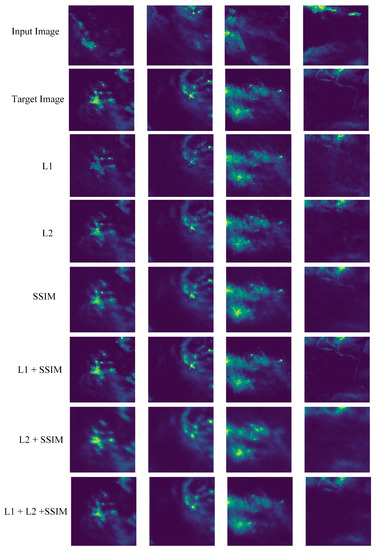
Figure 1.
Input and forecasted images for various regularization terms on Dataset-A for 4 h of lead time.
We compare the forecast accuracy of CGAN with the baselines U-Net and Persistence. As mentioned earlier, U-Net is also evaluated using different regularizations, but only the best values are reported in Figure 2 for space constraints. Figure 2a provides the test accuracy of models on Dataset-A. Notably, the reported results for CGAN are based on the L1 + SSIM regularization. Persistence shows a high POD, U-Net has a low FAR, and CGAN has a high SSIM on average. Persistence performs slightly better than CGAN in CSI, POD, and HSS for shorter lead times (up to one hour) because precipitation does not vary significantly in one hour, making it challenging to outperform Persistence. However, our CGAN model outperforms U-Net and Persistence in three out of five metrics for lead times greater than one hour. Additionally, CGAN and Persistence beat U-Net for all lead times in all metrics except FAR. Overall, CGAN scored 8, Persistence scored 7, and U-Net scored 5 out of 20 (five metrics × four lead times), demonstrating the capability of CGAN and the SSIM regularization.
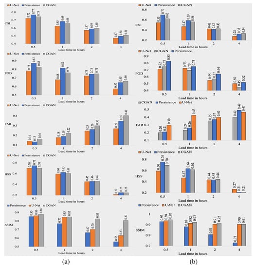
Figure 2.
Test accuracy of models trained with L1 and SSIM regularization for (a) Dataset-A, (b) Dataset-B measured using CSI, POD, FAR, HSS, and SSIM.
Figure 2b compares the test accuracy of models on Dataset-B. These results follow the same trend as Figure 2a. Overall, Persistence has a high POD, and CGAN has a low FAR and high SSIM. Furthermore, CGAN and Persistence outperform U-Net for almost all lead times and across all metrics. CGAN scored 12, and Persistence scored eight out of 20 (five metrics × four lead times), highlighting the capability of CGAN and SSIM regularization for precipitation nowcasting. An important observation from Figure 2a,b is that the POD (recall) for Dataset-B is lower than for Dataset-A at all lead times because of the fewer rainy pixels in Dataset-B than Dataset-A. This biases the CGAN model to forecast the majority of the pixels as no rain, indicating that CGAN can achieve higher accuracy in forecasting precipitation for longer lead times if more samples from the positive class (rainy pixels) are available.
6. Conclusions and Future Directions
This study demonstrates that using SSIM and mean absolute error (MAE, also known as L1) regularization in CGAN’s objective function can result in higher-quality predicted images, as measured by CSI, POD, FAR, HSS, and SSIM. Although the CSI, POD, and HSS for Dataset-B are lower than those for Dataset-A due to the smaller number of rainy pixels in Dataset-B, the proposed model can achieve higher forecast accuracy for larger datasets with more positive samples.
To evaluate the effectiveness of CGAN, we compared it with other baselines such as U-Net and Persistence. Persistence assumes that rainfall remains constant after a few hours, making it a difficult baseline to outperform in weather prediction, particularly for shorter lead times. Therefore, for up to one hour lead times, the CSI, POD, and HSS of Persistence are greater than those of CGAN and U-Net. However, for two hours and longer lead times, CGAN outperformed Persistence in terms of CSI, POD, and SSIM, demonstrating the superiority of CGAN and SSIM regularization in rainfall forecasting for longer lead times.
Author Contributions
Conceptualization, J.J. and M.H.; methodology, J.J.; formal analysis, J.J. and M.H.; writing—original draft preparation, J.J.; writing—review and editing, J.J. and M.H.; visualization, J.J. and M.H.; supervision, M.H.; project administration, J.J. All authors have read and agreed to the published version of the manuscript.
Funding
This research received no external funding.
Institutional Review Board Statement
Not applicable.
Informed Consent Statement
Not applicable.
Data Availability Statement
The data presented in this study are openly available in Github at https://github.com/jahnavijo/Data-for-Precipitation-Nowcasting.git.
Conflicts of Interest
The authors declare no conflict of interest.
References
- Guhatakurta, P.; Sreejith, O.P.; Menon, P.A. Impact of climate change on extreme rainfall events and flood risk in India. J. Earth Syst. Sci. 2011, 120, 359. [Google Scholar] [CrossRef]
- Srivastava, N.; Mansimov, E.; Salakhutdinowv, R. Unsupervised Learning of Video Representations using LSTMs. In Proceedings of the 32nd International Conference on Machine Learning, Lille, France, 6–11 July 2015; Volume 37, pp. 843–852. [Google Scholar]
- Tran, Q.-K.; Song, S.-K. Computer Vision in Precipitation Nowcasting: Applying Image Quality Assessment Metrics for Training Deep Neural Networks. Atmosphere 2019, 10, 244. [Google Scholar] [CrossRef]
- Klein, B.; Wolf, L.; Afek, Y. A Dynamic Convolutional Layer for Short Range Weather Prediction. In Proceedings of the IEEE Conference on Computer Vision and Pattern Recognition (CVPR), Boston, MA, USA, 7–12 June 2015. [Google Scholar]
- Mahdi, H.; Hassan, K. Weighted machine learning. Stat. Optim. Inf. Comput. 2018, 6, 497–525. [Google Scholar]
- Mahdi, H.; Hassan, K. Weighted machine learning for spatial-temporal data. IEEE J. Sel. Top. Appl. Earth Obs. Remote Sens. 2020, 13, 3066–3082. [Google Scholar]
- Jonnalagadda, J.; Hashemi, M. Feature Selection and Spatial-Temporal Forecast of Oceanic Nino Index Using Deep Learning. Int. J. Softw. Eng. Knowl. Eng. 2022, 32, 91–107. [Google Scholar] [CrossRef]
- Jonnalagadda, J.; Hashemi, M. Forecasting Atmospheric Visibility Using Auto Regressive Recurrent Neural Network. In Proceedings of the 2020 IEEE 21st International Conference on Information Reuse and Integration for Data Science (IRI), Las Vegas, NV, USA, 11–13 August 2020. [Google Scholar]
- Jonnalagadda, J.; Jahnavi; Hashemi, M. Spatial-Temporal Forecast of the probability distribution of Oceanic Niño Index for various lead times. In Proceedings of the 33rd International Conference on Software Engineering and Knowledge Engineering, Online, 1–10 July 2021; p. 309. [Google Scholar]
- Hashemi, M.; Alesheikh, A.A.; Zolfaghari, M.R. A GIS based time-dependent seismic source modeling of Northern Iran. Earthq. Eng. Eng. Vib. 2017, 16, 33–45. [Google Scholar] [CrossRef]
- Hashemi, M.; Alesheikh, A.A.; Zolfaghari, M.R. A spatio-temporal model for probabilistic seismic hazard zonation of Tehran. Comput. Geosci. 2013, 58, 8–18. [Google Scholar] [CrossRef]
- Balamurugan, M.S.; ManojKumar, R. Study of short term rain forecasting using machine learning based approach. Wirel. Netw. 2021, 27, 5429–5434. [Google Scholar] [CrossRef]
- Sangiorio, M.; Barindelli, S.; Guglieri, V.; Biondi, R.; Solazzo, E.; Realini, E.; Venuti, G.; Guariso, G. A Comparative Study on Machine Learning Techniques for Intense Convective Rainfall Events Forecasting. In Theory and Applications of Time Series Analysis: Selected Contributions from ITISE 2019; Springer: Cham, Switzerland, 2020; Volume 6, pp. 305–317. [Google Scholar]
- Pruden, R.; Adams, S.; Kangin, D.; Robinson, N.; Ravuri, S.; Mohammed, S.; Alberto, A. A review of radar-based nowcasting of precipitation and applicable machine learning techniques. arXiv 2020, arXiv:2005.04988. [Google Scholar]
- Agarwal, S.; Barrington, L.; Bromberg, C.; Burge, J.; Gazen, C.; Hickey, J. Machine Learning for Precipitation Nowcasting from Radar Images. In Proceedings of the 33rd Conference on Neural Information Processing Systems (NeurIPS 2019), Vancouver, BC, Canada, 8–14 December 2019. [Google Scholar]
- Trebing, K.; Tomasz, S.; Siamak, M. SmaAt-UNet: Precipitation nowcasting using a small attention-UNet architecture. Pattern Recognit. Lett. 2021, 145, 178–186. [Google Scholar] [CrossRef]
- Ayzel, G.; Scheffer, T.; Heistermann, M. RainNet v1.0: A con- volutional neural network for radar-based precipitation nowcasting. Geosci. Dev. 2020, 13, 2631–2644. [Google Scholar] [CrossRef]
- Yan, Q.; Ji, F.; Miao, K.; Wu, Q.; Xia, Y.; Teng, L. Convolutional Residual-Attention: A Deep Learning Approach for Precipitation Nowcasting. Adv. Meteorol. 2020, 2020, 6484812. [Google Scholar] [CrossRef]
- Kumar, A.; Islam, T.; Sekimoto, Y.; Mattmann, C. Convcast: An embedded convolutional LSTM based architecture for precipitation nowcasting using satellite data. PLoS ONE 2020, 15, e0230114. [Google Scholar] [CrossRef]
- Lei, C.; Yuan, C.; Ma, L.; Junping, Z. A Deep Learning-Based Methodology for Precipitation Nowcasting With Radar. Earth Space Sci. 2020, 7, e2019EA000812. [Google Scholar]
- Jeong, C.; Kim, W.; Joo, W.; Jang, D.; Yi, M. Enhancing the Encoding-Forecasting Model for Precipitation Nowcasting by Putting High Emphasis on the Latest Data of the Time Step. Atmosphere 2021, 12, 261. [Google Scholar] [CrossRef]
- Shi, X.; Chen, Z.; Wang, H.; Yeung, D.; Wong, W.; Woo, W. Convolutional LSTM Network: A Machine Learning Approach for Precipitation Nowcasting. Adv. Neural Inf. Process. Syst. 2015, 1, 802–810. [Google Scholar]
- Shi, X.; Gao, Z.; Lausen, L.; Wang, H.; Yeung, D.; Wong, W.; Woo, W. Deep Learning for Precipitation Nowcasting: A Benchmark and A New Model. In Proceedings of the 31st Conference on Neural Information Processing Systems, LongBeach, CA, USA, 4–9 December 2017. [Google Scholar]
- Zhang, C.; Yang, X.; Tang, Y.; Zhang, W. Learning to Generate Radar Image Sequences Using Two-Stage Generative Adversarial Networks. IEEE Geosci. Remote Sens. Lett. 2020, 17, 401–405. [Google Scholar] [CrossRef]
- Bihlo, A. A generative adversarial network approach to (ensemble) weather prediction. Neural Netw. 2021, 139, 1–16. [Google Scholar] [CrossRef]
- Choi, S.; Kim, Y. Rad-cGAN v1.0: Radar-based precipitation nowcasting model with conditional Generative Adversarial Networks for multiple domains. Geosci. Model Dev. 2020, 15, 5967–5985. [Google Scholar] [CrossRef]
- Hayatbini, N.; Kong, B.; Hsu, K.; Nguyen, P.; Sorooshian, S.; Stephens, G.; Fowlkes, C.; Nemani, R. Conditional generative adversarial networks (cGANs) for near real-time precipitation estimation from multispectral GOES-16 satellite imageries-PERSIANN-cGAN. Remote Sens. 2019, 11, 2193. [Google Scholar] [CrossRef]
- Huffman, G.J.; Stocker, E.F.; Bolvin, D.T.; Nelkin, E.J.; Tan, J. GPM IMERG Final Precipitation L3 Half Hourly 0.1 degree × 0.1 degree V06. Goddard Earth Sciences Data and Information Services Center (GES DISC): Greenbelt, MD, USA. Available online: https://disc.gsfc.nasa.gov/datasets/GPM_3IMERGHH_06/summary (accessed on 10 January 2022).
- Goodfellow, I.; Pouget-Abadie, J.; Mirza, M.; Xu, B.; Warde-Farley, D.; Ozair, S.; Courville, A.; Bengio, Y. Generative Adversarial Nets. Commun. ACM 2014, 63, 139–144. [Google Scholar] [CrossRef]
- Isola, P.; Zhu, J.; Zhou, T.; Efros, A.A. Image-to-Image Translation with Conditional Adversarial Networks. In Proceedings of the 2017 IEEE Conference on Computer Vision and Pattern Recognition (CVPR), Honolulu, HI, USA, 21–26 July 2017; pp. 5967–5976. [Google Scholar] [CrossRef]
- Wang, Z.; Bovik, A.C.; Sheikh, H.R.; Simoncelli, E.P. Image quality assessment: From error visibility to structural similarity. IEEE Trans. Image Process. 2004, 13, 600–612. [Google Scholar] [CrossRef] [PubMed]
- Zhao, H.; Gallo, O.; Frosio, I.; Kautz, J. Loss functions for image restoration with neural networks. IEEE Trans. Comput. 2016, 3, 47–57. [Google Scholar] [CrossRef]
- Kancharla, P.; Channappayya, S.S. Quality Aware Generative Adversarial Networks. In Proceedings of the 33rd Conference on Neural Information Processing Systems, Vancouver, BC, Canada, 8–14 December 2019. [Google Scholar]


Disclaimer/Publisher’s Note: The statements, opinions and data contained in all publications are solely those of the individual author(s) and contributor(s) and not of MDPI and/or the editor(s). MDPI and/or the editor(s) disclaim responsibility for any injury to people or property resulting from any ideas, methods, instructions or products referred to in the content. |
© 2023 by the authors. Licensee MDPI, Basel, Switzerland. This article is an open access article distributed under the terms and conditions of the Creative Commons Attribution (CC BY) license (https://creativecommons.org/licenses/by/4.0/).