A Time Series Autoencoder for Load Identification via Dimensionality Reduction of Sensor Recordings ^†

Abstract

Current progress in sensor technology is setting the ground to push toward satisfactory solutions to challenging engineering problems, like e.g., system identification and Structural Health Monitoring (SHM). In civil engineering, SHM is often based on the analysis of vibrational recordings, represented by time histories of displacements and/or accelerations, collected through pervasive sensor networks and shaped as Multivariate Time Series (MTS). Despite the great advances in soft computing techniques such as neural networks, inverse problems featuring regression tasks on raw vibrational measurements are still challenging. Developing dimensionality reduction tools, able to infer complex correlations within and across the recorded time series, is then of paramount importance. In this work, we designed an AutoEncoder (AE) capable of condensing MTS-shaped data in a reduced format featuring a few latent variables only. The obtained reduced data representation enhances the solution of inverse problems, like e.g., the identification of the parameters governing the dynamic load applied to a structural system. Numerical examples, aimed at the identification of the loading conditions on a shear-type building, are reported to assess the effectiveness of the proposed procedure.

1. Introduction

Data collected by pervasive sensor networks have to be processed, since they are usually unmanageable in their raw forms. Their dimension is the principal obstacle making their use extremely difficult, while the information content is typically highly redundant. Synthetic features like spectral peak frequencies, usually exploited when the acquired data are shaped as Time Series (TS), are extracted to solve engineering tasks, like load identification and Structural Health Monitoring (SHM) [1,2]. Deep Learning (DL) allows extracting features from the data according to the required task, avoiding any preliminar feature design [3,4,5,6]. Among DL techniques, AutoEncoders (AEs) are special type of Neural Networks (NN) able to obtain a reduced data representation [7], also called latent representation, without specifying the task the reduced data representation must be used for.

The NN architecture employed by an AE is usually deep or, in other words, involves the use of multiple sequential transformations. The advantages of employing AEs are manifold: (i) no feature engineering is necessary; (ii) the obtained reduced data representation can be used for different tasks; (iii) they provide the most informative data representation by setting the number of latent variables or, at least, the one that allows to reconstruct data at best. Thanks to their reduced number, latent variables are often interpretable, but only at the price of knowing something about what stays behind the variability of the collected data [8].

In the following, a novel TS AE is proposed for the dimensionality reduction of the pseudo-experimental Multivariate Time Series (MTSs) recordings related to the displacement response of a two-storey shear building. The effectiveness of the dimensionality reduction is judged by the AE ability of reconstructing the input signals from their latent representation. Despite the lack of any a priori performed task-oriented feature engineering, the obtained reduced data representation allows the identification of the load conditions applied to the building.

2. Methodology: A Deep Autoencoder for Load Identification

A Neural Network (NN) is a collection of units, called neurons. Each neuron performs, in its basic form, a linear combination of its input $\mathcal{V}\in {\mathbb{R}}^L$ (which reads ${\mathbf{v}}_b$ for the AE input channels, see below) via a weight vector $\omega$, and applies a nonlinear activation function $\zeta$. If a set of L neurons, called layer, is applied to $\mathcal{V}$, the output becomes a vector $\mathcal{U}\left(\mathcal{V},\Omega \right)\in {\mathbb{R}}^L$, where $\Omega =\left[{\omega }_1,\dots ,{\omega }_L\right]$. Many layers can be stacked one after another, making the NN architecture deep.

A special type of NN layer is the convolutional one, which allows to infer correlations within and across the inputs, whenever the inputs are shaped as a collection of one-dimensional arrays. In this work, the inputs are a set of MTSs $\mathbf{v}=\left[{\mathbf{v}}_1,\dots ,{\mathbf{v}}_N\right]\in {\mathbb{R}}^{L\times N}$ acquired by a sensor system employing N sensors, and sampling L displacement recordings within a time interval $\left(0,T\right)$. The output $\mathbf{U}\left(\mathbf{V},\Omega \right)=\left[{\mathbf{u}}_1,\dots ,{\mathbf{u}}_{N^{out}}\right]$ of a one-dimensional convolutional layer then reads

$${\mathbf{u}}_n\left(\mathbf{V},{\Omega }_n\right)=\sum _{b=1}^N{\omega }_n^b\ast {\mathbf{v}}_b,n=1,\dots ,N^{out},$$

(1)

where: $\ast :\left({\mathbb{R}}^{H_{out}}\times {\mathbb{R}}^L\right)\to {\mathbb{R}}^L$ is the discrete convolution operator [9]; ${\Omega }_n=\left[{\omega }_n^1,\dots ,{\omega }_n^N\right]\in {\mathbb{R}}^{H^{out}\times N}$ are the weights applied to ${\mathbf{v}}_b$ (with $b=1,\dots ,N$); $\Omega =\left[{\Omega }_1,\dots ,{\Omega }_{N^{out}}\right]\in {\mathbb{R}}^{H^{out}\times N\times N^{out}}$ collects all the layer weights; $H^{out}$ is the kernel dimension; N also represents the number of channels of the input layer; $N^{out}$ is the number of channels of the output layer.

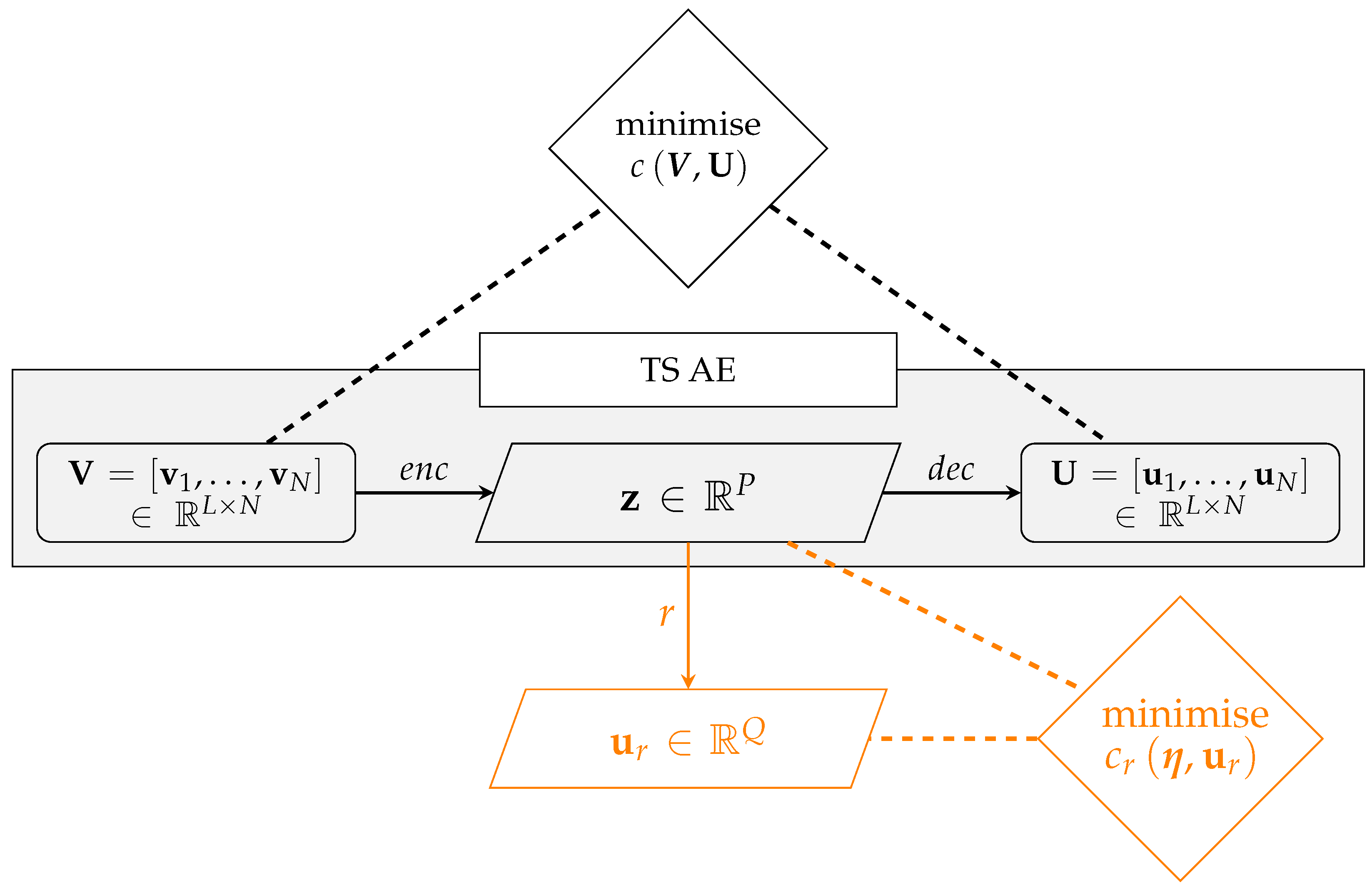
One-dimensional convolutional layers are the building blocks of the proposed AE. This latter is composed by an encoder $enc$ and by a decoder $dec$. The encoder maps the input $\mathbf{V}$ into a latent representation $\mathbf{z}=\mathbf{z}\left(\mathbf{V}\right)\in {\mathbb{R}}^P$, with $P\ll \left(L\times N\right)$, while the decoder maps $\mathbf{z}$ into a two dimensional array $\mathbf{U}=\mathbf{U}\left(\mathbf{z}\right)\in {\mathbb{R}}^{L\times N}$. Being $\mathbf{U}$ shaped as $\mathbf{V}$, we can enforce the AE to reconstruct $\mathbf{V}$ from $\mathbf{z}$ by defining

$$c\left(\mathbf{V},\mathbf{U}\right)=\sum _{l=1}^L\sum _{n=1}^N{\left(v_{ln}-u_{ln}\right)}^2,$$

(2)

as loss function to be minimised by the NN during the training, which consists in tuning the weights $\Omega$ ruling the layer operations.

The latent representation $\mathbf{z}$ can be used to solve a regression problem, involving the identification of the parameter vector $\eta \in {\mathbb{R}}^Q$ e.g., governing the loadings applied to the structure. If the decoder can (almost perfectly) reconstruct $\mathbf{V}$ starting from $\mathbf{z}$, it means that $\mathbf{z}$ condenses all the relevant informations of $\mathbf{V}$. As shown in Figure 1, a NN-based regression model r is employed to retrieve $\eta$ starting from $\mathbf{z}$, accomplishing this way the load identification task. To train r, a loss function $c_r\left(\eta ,{\mathbf{u}}_r\right)$ is defined as done in Equation (2), where ${\mathbf{u}}_r\in {\mathbb{R}}^Q$ is the prediction of r. The training of the AE and of r takes place sequentially, first minimising $c\left(\mathbf{V},\mathbf{U}\right)$, and then minimising $c_r\left(\eta ,{\mathbf{u}}_r\right)$. A popular first-order stochastic gradient descend algorithm, called Adam [10], has been employed for these procedure tasks.

3. Results and Discussion

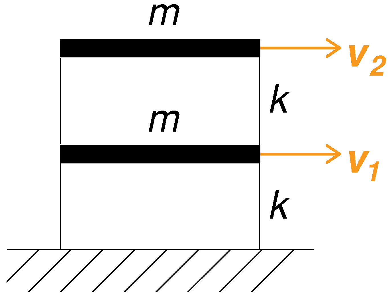
The lateral displacements of a two-storey building, shown in Figure 2, are monitored by a sensor system employing two sensors (one per floor), recording L samples within the time window $\left(0,T\right)$. Then, the output of the monitoring system is an MTS $\mathbf{V}\in {\mathbb{R}}^{L\times N}$, with $L=250$ and $N=2$. The dynamic response of the structure is simulated by means of a two-dimensional shear building model wherein, due to the mass distribution and load bearing elements, torsional effects have been disregarded. Damping has not been modelled, having a negligible effect on the identification of continuously excited structures [11,12]. We assumed that the applied lateral loads consist of forces enforced at the floor levels, featuring a sinusoidal time dependence, ruled by the parameter $\varphi$, and a linearly increasing amplitude along the building height, governed by the parameter $\alpha$, i.e.$A_c=0.5c\alpha \sin \left(2\pi \varphi t\right)$ with $c=1,2$. Therefore, the parameter vector $\eta =\{\alpha ,\varphi \}$ looks sufficient to fully describe the loading conditions. A uniform probability density function was associated with each parameter: ${\mathcal{U}}_{\alpha }\left(\alpha \right)=\frac{1}{\left(6.25-0.625\right){10}^3\mathrm{N}}$ for $\alpha$, and ${\mathcal{U}}_{\varphi }\left(\varphi \right)=\frac{1}{\left(15-1\right)\mathrm{Hz}}$ for $\varphi$. Regarding the structural properties of the building, the same values of mass $m=625\mathrm{ton}$ and interstory stiffness $k={10}^6$$\frac{\mathrm{kN}}{\mathrm{m}}$ have been assumed for the two floors. Consequently, the resonance frequencies of the building are ${\mathbf{f}}^{str}=\left[3.93,10.3\right]\mathrm{Hz}$, while the structural periods are ${\mathbf{T}}^{str}=\left[0.255,97.1·{10}^{-3}\right]\mathrm{s}$.

A dataset, collecting $12,000$ MTSs, has been assembled to train the AE and r; 4000 additional MTSs, forming the validation set, have been then employed to avoid overfitting. The training dataset is processed several times, or epochs. If the loss function computed with the validation set has not reduced for 50 epochs in a row, the training has been early stopped. A test set, gathering 512 MTSs, has been then employed to verify the reconstruction capacity of the AE, and the performance of the proposed load identification procedure. The reconstruction capacity has been evaluated through two error measures, employing either a standardised $L^2$ norm or a standardised $L^{\infty }$ norm. The error measures have been computed for each reconstructed signal, and standardisation has been done by dividing the reconstruction error (either the $L^2$ or $L^{\infty }$ norm) by the standard deviation of the original signal. Without standardisation, small inaccuracies in reconstructing large displacements would have counted more than large inaccuracies at smaller scales.

A thorough investigation has been carried out to study how the number P of latent variables and the parameter $\varphi$ ruling the time dependence of loading, affect the reconstruction capacity of the AE; the other way around, no correlation between the reconstruction error and $\alpha$ has been found in our experiments. Indeed, the mean value and the spread of the reconstruction error can not be modelled as a function of $\alpha$, but rather as a function of $\varphi$. 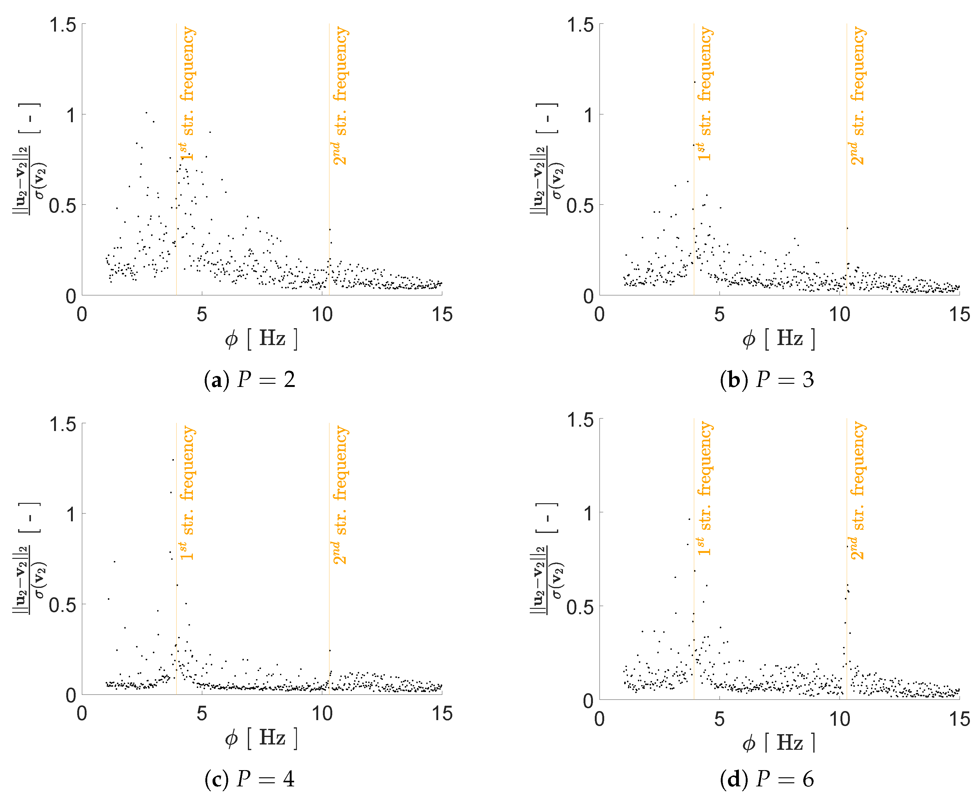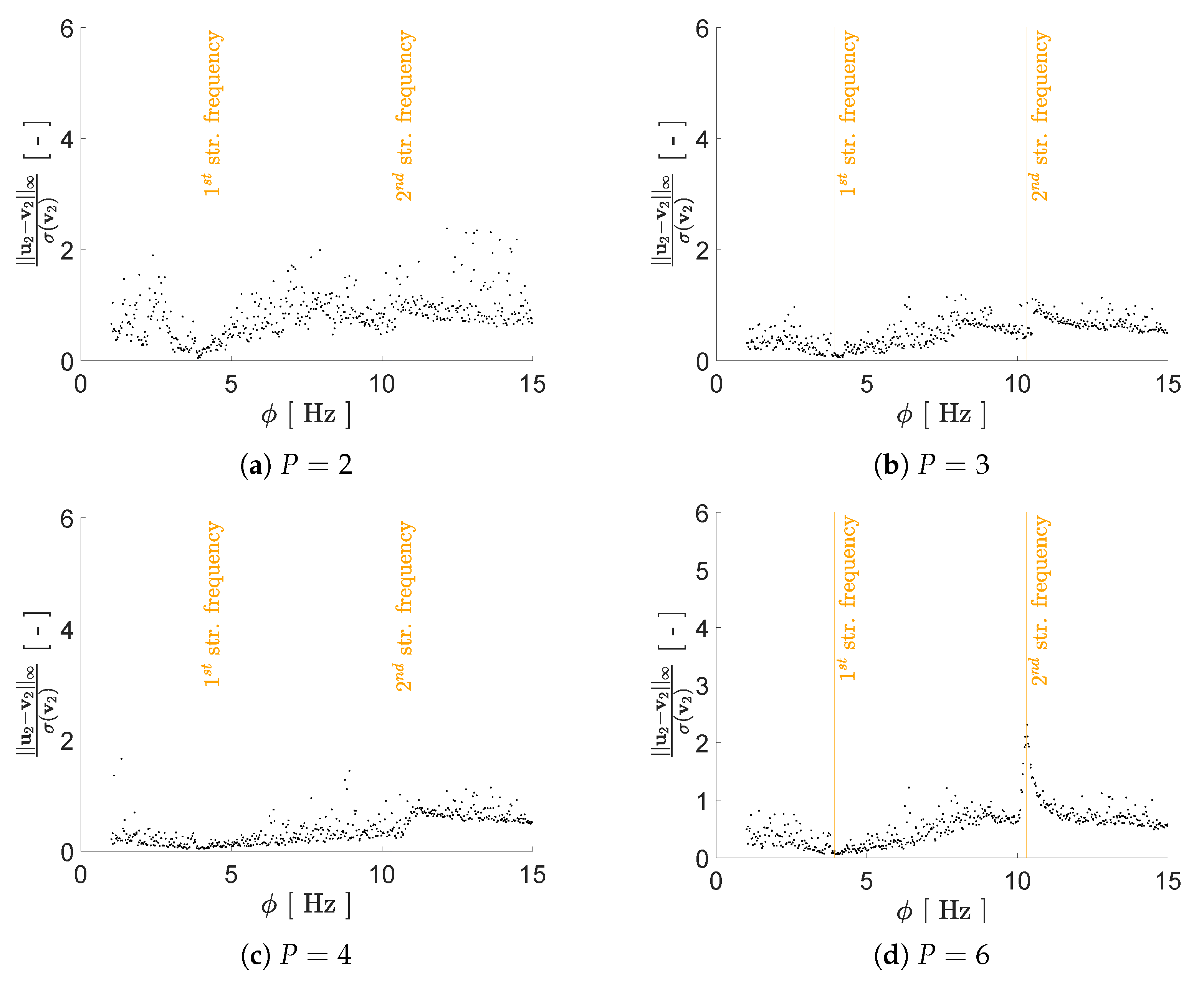Figure 3 and Figure 4 depict the reconstruction error measured, respectively, by the standardised $L^2$ and $L^{\infty }$ norms, when the input signals have been taken from the test set. The graphs for $P=5$ (not reported for brevity) are analogous to those obtained for $P=6$, even if showing slightly higher values of the reconstruction error. An increasing value of P does not lead to a monotonic enhancement of the AE reconstruction capacity, despite the intuition that a larger latent space should make reconstruction easier. Indeed, even if increasing the value of P has not led to retain more information on the system, we do expect that a more redundant representation should not be detrimental.

A clear relation between the error and $\varphi$ can be underlined. Looking at the standardised $L^2$ norm, the reconstruction capacity of the AE seems worse when $\varphi \approx f_1^{str}$ and $\varphi \approx f_2^{str}$. This result is not surprising: the beats produced in the displacement recordings, when $\varphi$ is close to the structural frequencies of the building, are additional signal characteristics that the AE must struggle to account for. Focusing on the standardised $L^{\infty }$ norm, the reconstruction error is still large for $\varphi \approx f_2^{str}$, while it gets smaller for $\varphi \approx f_1^{str}$.

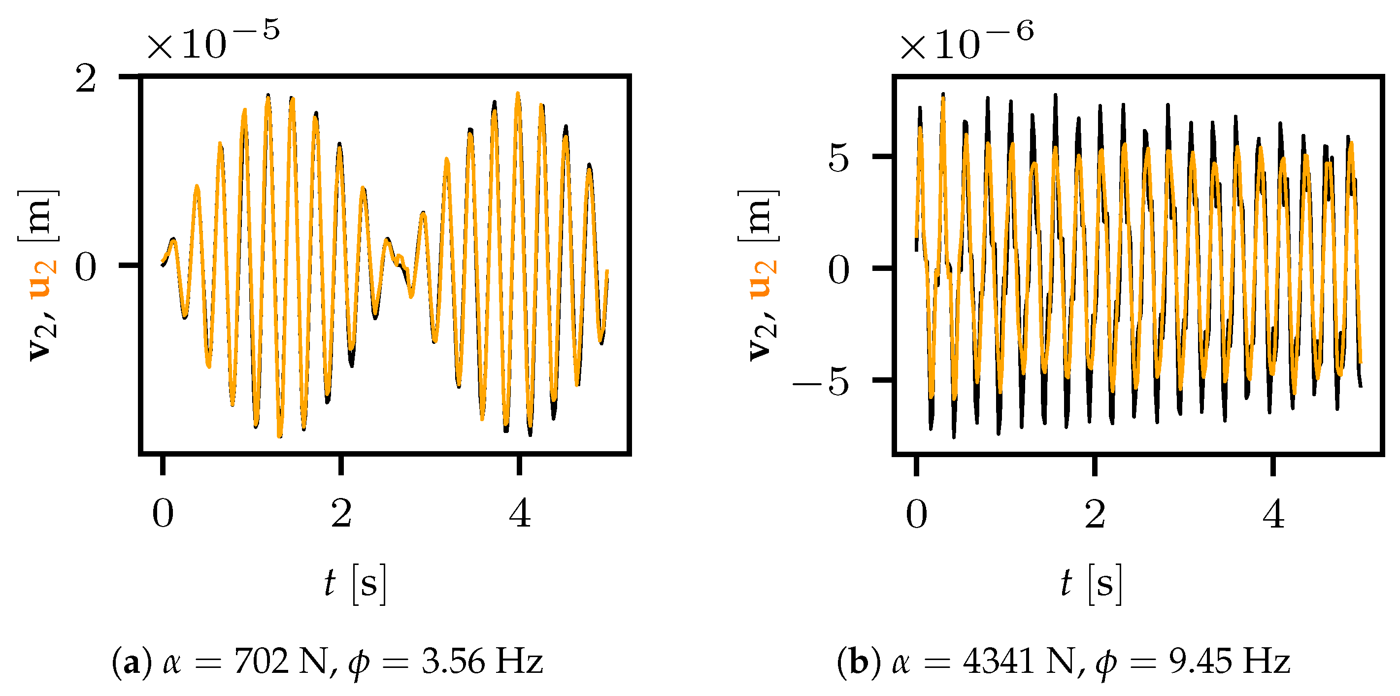
In Figure 5, a qualitative assessment of the reconstruction capacity of the AE is reported, to better highlight the meaning of the two error norms: the good signal reconstruction obtained for $\varphi ⪅f_1^{str}$ points toward the $L^{\infty }$ norm as a more appropriate error measure. On the other hand, we are convinced that both these error measures give meaningful information, because the standardised $L^2$ norm addresses inaccuracies in reproducing the frequency content of the input signal, while the standardised $L^{\infty }$ norm highlights the inability of catching its peaks. Still referring to Figure 5, we observe that the amplitude of the signal in Figure 5a is an order of magnitude greater than the one in Figure 5b, despite $\alpha =702\mathrm{N}$ in the first case, and $\alpha =4341\mathrm{N}$ in the second case. The reason is that we are exciting an undamped dynamic system with $\varphi$ closer to $f_1^{str}$ in Figure 5a than to $f_2^{str}$ in Figure 5b.

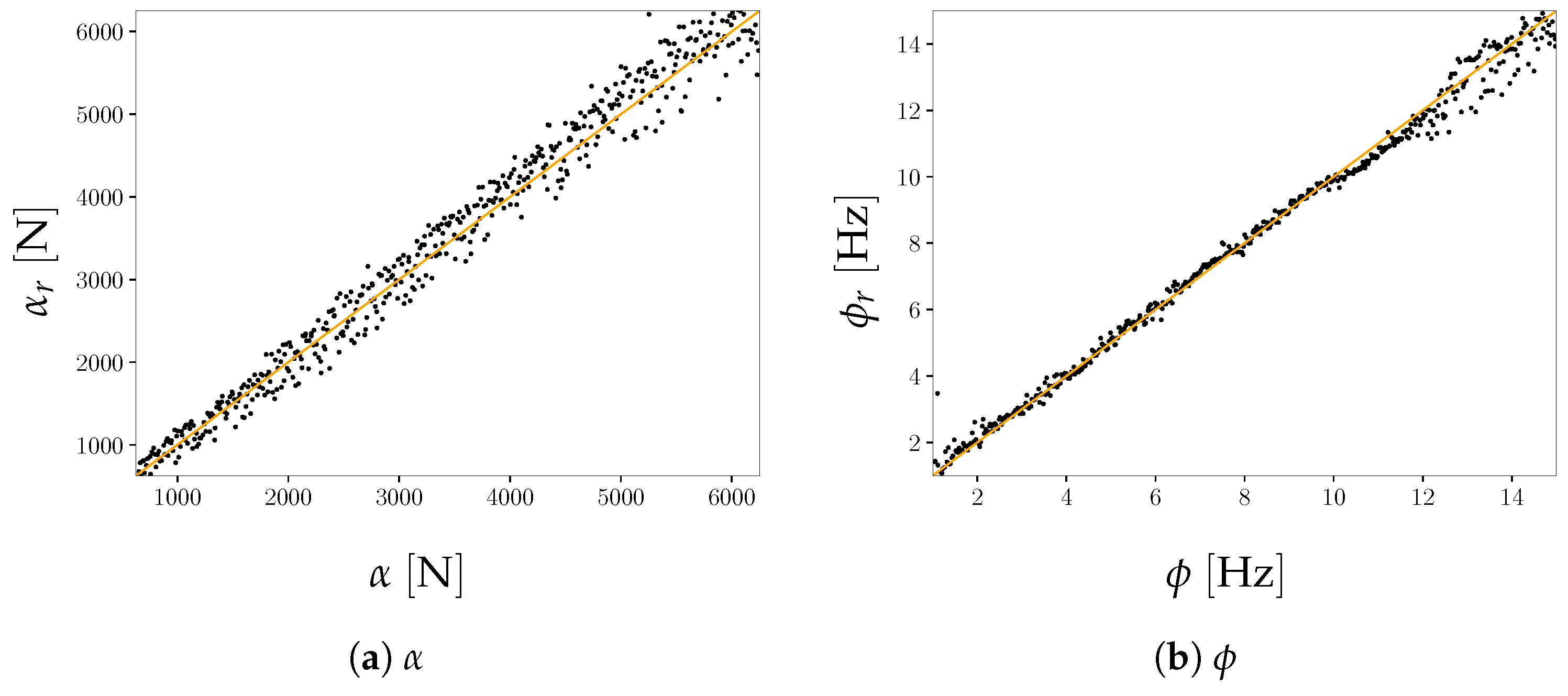
On the basis of the obtained latent representation $\mathbf{z}$, we performed the regression of the parameters $\eta$ governing the loading conditions. As shown in Figure 6b, the regression of the load frequency $\varphi$ has been rather successfully accomplished: the graph has been obtained with the latent space dimension featuring the highest reconstruction capacity, linked to $P=4$. An analogous result has been obtained for the regression of the load amplitude $\alpha$, shown in Figure 6b, confirming that the proposed strategy, involving dimensionality reduction of the input and the use of a regression model, allows a correct load identification for the case at hand. It is also worth mentioning that the largest errors in the $\varphi$ prediction have been obtained for the frequency range featuring the highest reconstruction error in the $L^{\infty }$ norm.

4. Conclusions

The use of a time series autoencoder was proposed for the dimensionality reduction of sensor recordings, typically acquired for the SHM of civil structures. Thanks to the obtained latent representation, the regression of the parameters governing the loading conditions can be successfully carried out. Two error norms have been used to quantitatively assess the signal reconstruction capacity of the autoencoder, evaluated for different dimensions of the latent space. The capability of the autoencoder to reconstruct the input signals has been assessed also qualitatively, through comparison of the input and reconstructed signals in the less accurate cases.

In future works, we aim to understand the role of the latent space dimension on the autoencoder reconstruction capacity, and to investigate how to set it automatically and optimally.