Deep Learning for the Prediction of Temperature Time Series in the Lining of an Electric Arc Furnace for Structural Health Monitoring at Cerro Matoso (CMSA) ^†

Abstract

Cerro Matoso SA (CMSA) is located in Montelibano, Colombia. It is one of the biggest producers of ferronickel in the world. The structural health monitoring process performed in the electric arc furnaces at CMSA is of great importance in the maintenance and control of ferronickel production. The control of thermal and dimensional conditions of the electric furnace aims to detect and prevent failures that may affect its physical integrity. A network of thermocouples distributed radially and at different heights from the furnace wall, are responsible for monitoring the temperatures in the electric furnace lining. In order to optimize the operation of the electric furnace, it is important to predict the temperature at some points. However, this can be difficult due the number of variables which it depends on. To predict the temperature behavior in the electric furnace lining, a deep learning model for time series prediction has been developed. Long Short Term Memory (LSTM), Gated Recurrent Unit (GRU), and other combinations were tested. GRU characterized by its multivariate and multi output type had the lowest square error. A study of the best input variables for the model that influence the temperature behavior is also carried out. Some of the input variables are the power, current, impedance, calcine chemistry, temperature history, among others. The methodology to tune the parameters of the GRU deep learning model is described. Results show an excellent behavior for predicting the temperatures 6 h into the future with root mean square errors of 3%. This model will be integrated to a software that obtains data for a time window from the Distributed Control System (DCS) to feed the model. In addition, this software will have a graphical user interface used by the operators furnace in the control room. Results of this work will improve the process of structural control and health monitoring at CMSA.

1. Introduction

Electric arc furnace (EAF) is a kind of furnace that heats materials by the covered-arc smelting process. The efficiency of these furnaces depends on the control and prediction of some variables such as power, temperature of the furnace, feed delivered, calcine composition, and others [1]. Some EAF work in the order of Mega Volt-Amperes which means any improvement in efficiency represents energy savings [2].

Analytical techniques have been used traditionally in EAF models to predict temperature and other variables [3]. These models have a low computational load to be implemented, however, they present problems when many input variables are included. Autoregressive models have been used in EAF models [4] with interesting results. Nonetheless, the processes of parameter estimation are generally not adaptive [5], since an EAF is a complex and nonlinear system. In the recent decade, some machine learning techniques such as artificial neural networks [2], fuzzy logic [6], deep learning [7], and others, have been used to model EAF and estimate temperature, power, voltage flickering, and other variables. Some of the advantages of these techniques are adaptive behavior, multiple input and output variables, learning of hidden patterns, and others [7].

Cerro Matoso SA in Montelibano (Colombia) is one of the biggest producers of ferronickel in the world and features two 75MW electric arc furnaces. A set of sensors along the furnaces monitor temperature, calcine composition, power, and other variables. These variables are used to monitor the furnace operation and select appropriate control parameters [1]. This paper presents a deep learning model to predict temperature for a electric arc furnace in Cerro Matoso SA (CMSA). In order to select an appropriate method, Convolutional Networks, Long Short Term Memory Networks, and Gated Recurrent Unit Networks were tested. In addition, multimodal methods were considered by implementing combinations of these three techniques.

The paper is organized as follows, Section 2 describes the electric arc furnace operation, data employed, and the methods used to predict the temperatures, Section 3 shows the results and the considerations taken to compare the different methods, and Section 4 gives the conclusions.

2. Materials and Methods

2.1. Data

The source of data for this research consisted of a 4-year sample of data, in the interval of time from September 2015 to September 2019, containing electric arc furnace operational information, like operational information and calcine and slag chemistry information. The data set was cleaned in order to remove the values that were deemed atypical, according to the team of operational experts at CMSA, and the main cause for the atypical values was the malfunction of some of the sensors caused by the harsh conditions inside the furnace. The parameters selected to predict the temperature in the furnace were the following:

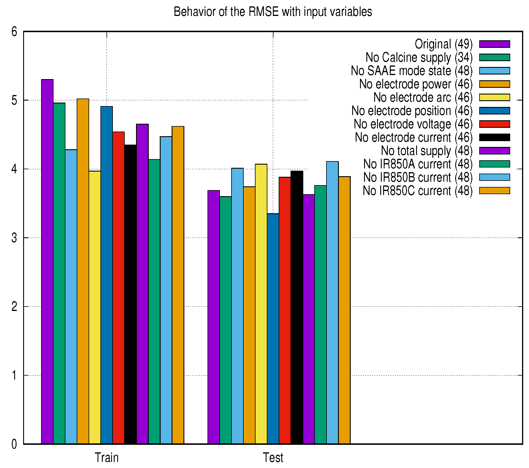
• Input variables: 49 input variables consisting of electrode current, electrode voltage, electrode relative position, electrode arc, electric oven power, electrode power, electrode current, total feeding calcine by hour, calcine chemical composition, and thermocouple temperature by furnace sector and position.
• Time period: Each one of the input variables was sampled using a 15-min window.
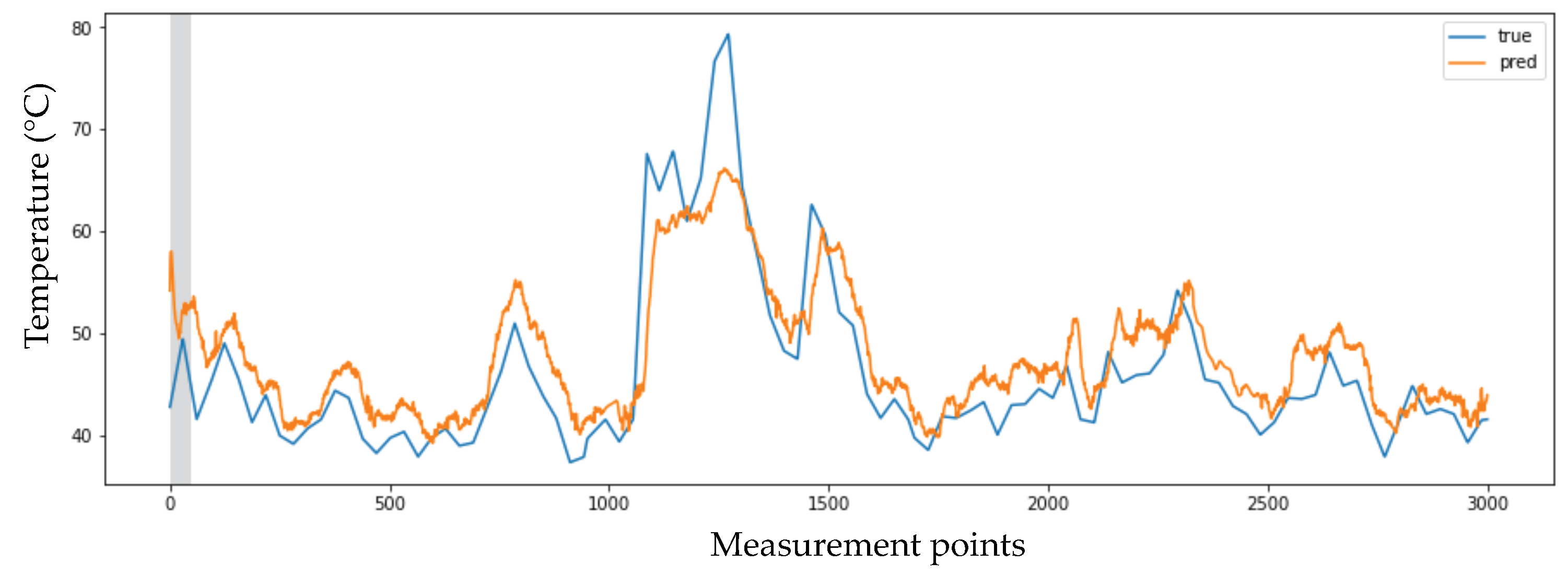
• Output variables: 16 output variables refer to 16 thermocouples distributed radially every 90 degrees in the furnace in four groups and spaced at four different heights of the furnace lining.

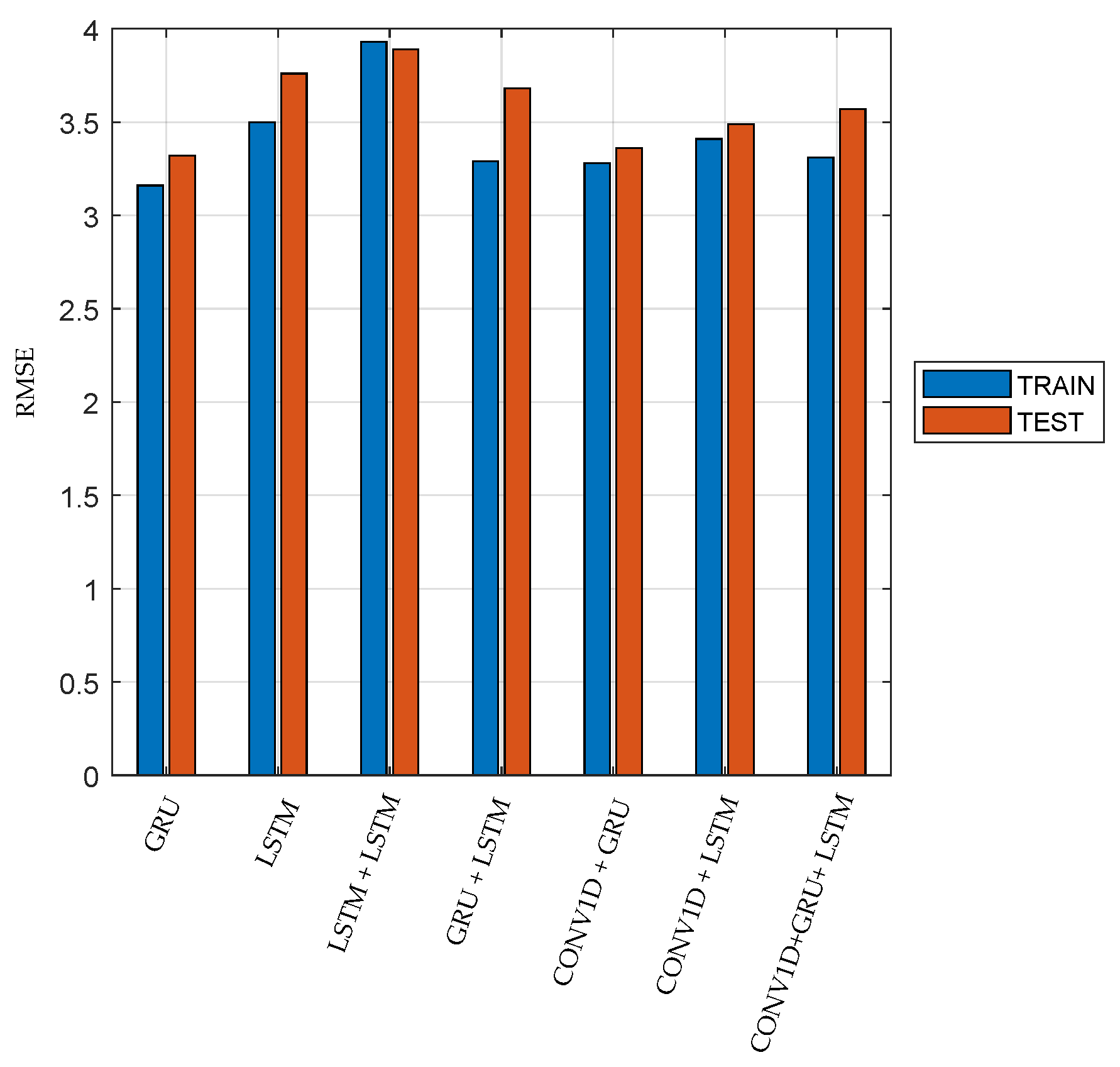
2.2. Predictive Methods

Deep Learning Recurrent Neural Networks. Deep learning architectures such as Convolutional Neural Networks (CNN) and Recurrent Neural Networks (RNN), and a combination of both models are used to discover hidden relationships and structures in high dimensional data. Deep learning neural networks can automatically learn complex arbitrary input-to-output assignments and support multiple inputs and outputs. These features are suitable for time series forecasting, particularly in problems with complex nonlinear dependencies, multivalent inputs, and to produce multi-step forecasts. These characteristics offer many real world applications, such as complex classification problems, text categorization, computer vision, image processing, and speech recognition [8].

Convolutional Neural Networks (CNNs) have a similar architecture to a feed-forward artificial neural network, but they diverge in terms of how is implemented the connectivity patterns between neurons in adjacent layers, and the CNN reduces the parameter scale in the model by using a specialized layer called the pool layer, and the final layer is the only one that is fully connected [9]. CNNs are employed directly on raw data, such as raw pixel values, instead of domain-specific or characteristics derived from the raw data. The model then learns how to automatically extract characteristics from the raw data, this process of learning is called representation learning, and CNN accomplishes this in such a way that features are extracted regardless of how often they occur in the data, the so-called transform or distortion invariance.

Long Short Term Memory network (LSTM) architecture adds to the CNN model the explicit handling of the order between observations when learning an input-to-output mapping function, in a manner not offered by other methods such as MLP or CNN. LSTM is a type of neural network that adds native support for input data composed of sequences of observations. Instead of assigning inputs to outputs alone, LSTM is able to learn a mapping function for inputs over time to an output. This LSTM capability has been used to great effect in complex Natural Language Processing (NLP) problems, such as neural machine translation, and can be used in time series forecasts, by automatically learning the time dependence of data [10,11].

Gated Recurrent Unit (GRU). GRU is a recursive convolutional network where the parameters at each level are shared through the entire network [12], configuring a convolutional network architecture implementing a gating mechanism, employing update and reset gates, that applies recursively the network weights to the input sequence until it outputs a single fixed-length vector. The gating mechanism allows the GRU to learn the structure of the input data.

2.3. Development of the Deep Learning Models

The input and output signals are defined along with the data split percentages for the training and test sets. The data set contains a wide range of values and the neural network works best at values between approximately 0 and 1, so the data must be scaled before it is entered into the neural network. The total data set consists of 40,000 observations, the training percentage was defined at 90% and the remaining 10% for testing. Furthermore, 49 input variables and 16 output variables were used.

The training data have 36,000 observations. Instead of training the Recurrent Neural Network on the entire sequences, a function will be used to create a batch of shorter subsequences (batches), randomly selected from the training data. We will use a sequence length of 1152 steps, which means that each random sequence contains observations of 12 days. One time step corresponds to 15 min.

The batch generator randomly selects a batch of short sequences from the training data and uses it during training. For the validation data, the entire sequence was run from the test set and the prediction precision was measured on that entire sequence.

Due to its simplicity, Keras API was used for creating the Recurrent Neural Network (RNN). In addition, a sequential model build was used. The number of cells for the different deep neural networks were 32 for CONV1D, 100 for GRU, 32 for the first layer of LSTM, and 16 for the second layer of LSTM. For the first layer in the model, Keras needs to know the shape of its input, which is a batch of sequences of arbitrary length (indicated by ’None’), where each observation has several input signals ($num-x-signals$).

The Gated Recurrent Unit (GRU) has 100 exits for each time step in the sequence.We want to predict 16 output signals, so we added a fully connected (or dense) layer that maps 100 values to only 16 values. The output signals in the data set have been limited to values between 0 and 1 using a scalar object. Therefore, we also limited the output of the neural network using the Sigmoid trigger function, which forces the output to be between 0 and 1.

The root mean square error (RMSE) was used as the loss function to be minimized. This function measures how closely the model output matches the true output signals. However, at the beginning of a sequence, the model has only observed input signals for a few time steps, so its generated output can be very imprecise. Using the loss value in the first time steps can cause the model to distort its later output. Therefore, we gave the model a “warm-up-period” of 50 time steps without using its precision in the stall function, hoping to improve accuracy in subsequent time steps. The root mean square error was calculated between $y-true$ and $y-pred$, but the initial “warm-up” part of the sequences was ignored. The learning rate for the optimizer is reduced if the loss of validation has not improved since the last epoch. The learning rate will be reduced by multiplying it by the given factor. We set an initial learning rate of $1\times {10}^{-3}$ above, so multiplying it by 0.1 gives a learning rate of $1\times {10}^{-4}$. The learning rate should not be lower than this.

3. Results

Different configurations of deep neural networks were trained and tested. As a result that there were 16 temperature output variables, an average root mean square error was calculated for each deep learning model. The deep learning models trained and tested were: GRU, LSTM, 2 layers of LSTM, GRU + LSTM, CONV1D + GRU, CONV1D + LSTM, and CONV1D + GRU + LSTM. As shown in Figure 1, the best model was the one that used only the GRU network.

In order to determine the behavior of the models in relation to the different input variables, different tests were carried out using the GRU model and limiting the number of input variables. The results obtained are shown in Figure 2. Figure 2 shows that, in the training process, the mean square error values decrease to a greater extent when the arc variables are eliminated in the electrode. Additionally, the best behavior in the test set occurs if we eliminate the variables corresponding to the electrode position.

Table 1. RMSE results in the 16 thermocouples for the train and test sets versus the different deep learning models.

	GRU		LSTM		LSTM+ LSTM		GRU+ LSTM		CONV1D+ GRU		CONV1D+ LSTM		CONV1D+ GRU + LSTM
Thermocouple (T)	Train	Test	Train	Test	Train	Test	Train	Test	Train	Test	Train	Test	Train	Test
T1 (L4,NW) (42.05 ± 5.18)	2.14	4.03	2.43	5.21	2.42	5.07	2.15	4.50	2.08	4.19	2.29	4.98	2.15	4.44
T2 (L4,SW) (47.73 ± 6.82)	2.73	3.70	3.13	4.22	3.16	4.05	2.73	4.12	2.86	3.82	3.04	4.21	2.81	3.80
T3 (L4,SE) (45.19 ± 3.23)	2.25	2.51	2.40	3.05	2.52	3.04	2.23	2.88	2.23	2.46	2.27	2.69	2.23	2.63
T4 (L4,NE) (41.88 ± 2.82)	1.46	1.23	1.66	1.35	1.75	1.58	1.47	1.31	1.46	1.26	1.64	1.21	1.53	1.55
T5 (L3,NW) (48.86 ± 9.71)	3.45	4.65	3.89	5.85	3.76	5.68	3.36	5.05	3.21	4.47	3.63	5.33	3.41	4.47
T6 (L3,SW) (54.08 ± 10.33)	3.72	4.70	4.67	5.24	4.56	4.98	3.87	5.51	3.98	5.56	4.23	4.99	4.08	5.77
T7 (L3,SE) (46.65 ±  4.69)	2.57	3.81	2.76	4.53	2.89	4.15	2.47	3.68	2.61	3.73	2.71	3.70	2.57	3.57
T8 (L3,NE) (42.23 ± 3.37)	1.66	1.41	1.83	1.55	1.90	1.75	1.72	1.40	1.64	1.51	1.73	1.32	1.67	1.54
T9 (L2,NW) (50.13 ±  6.92)	2.40	2.49	2.77	2.82	2.80	3.20	2.41	2.53	2.31	2.28	2.59	2.65	2.40	2.54
T10 (L2,SW) (53.70 ± 6.92)	2.59	2.34	3.29	2.93	3.08	2.78	2.64	2.55	2.73	2.50	2.85	2.38	2.86	2.84
T11 (L2,SE) (49.32 ± 4.96)	2.52	3.02	2.91	3.62	2.90	3.55	2.52	3.18	2.65	3.19	2.80	3.43	2.59	3.61
T12 (L2,NE) (44.72 ± 3.65)	1.70	1.77	1.94	1.52	1.87	2.00	1.70	1.78	1.69	1.87	1.77	1.85	1.71	1.99
T13 (L1,NW) (75.21 ± 18.32)	7.58	8.64	8.76	9.52	8.29	9.02	7.68	10.11	7.56	7.96	8.14	9.40	7.54	8.70
T14 (L1,SW) (81.17 ± 18.72)	6.84	7.24	8.66	9.30	8.09	7.98	6.96	7.40	7.03	7.37	7.50	7.14	7.39	7.95
T15 (L1,SE) (64.96 ± 9.44)	4.24	6.07	5.35	7.08	5.20	6.81	4.37	6.37	4.62	5.96	4.70	6.74	4.49	6.60
T16 (L1,SE) (58.86 ± 7.39)	2.92	3.80	3.62	3.01	3.40	4.34	3.06	4.26	3.05	4.62	3.19	3.84	3.14	4.57

shows the results of the root mean square error for each of the 16 thermocouples and the different deep learning models used in the train and test sets. The thermocouples are located at 4 different levels, level 4 being the highest and level 1 the lowest.

As results of the GRU model evaluation, a comparison of the predicted and true behaviors for one thermocuple in the test set is shown in Figure 3. An RMSE of 4.06 Celsius degrees was obtained in the 3000 measurements for the GRU model.

==layoutwidth=297mm,layoutheight=210 mm, left=2.7cm,right=2.7cm,top=1.8cm,bottom=1.5cm, includehead,includefoot [LO,RE]0cm [RO,LE]0cm

==

4. Discussion

Different time series deep learning models were developed to predict the temperature behavior in an electric furnace. The best model was GRU due to its low RMSE compared to other models like LSTM, CONV1D, and combinations between them. The study allowed identifying the input variables that best contribute to the prediction of temperatures. As future work, it is desired to automate the training process of a new neural network every certain period of time.

5. Conclusions

Different models of deep learning of time series were developed to predict the behavior of the temperature in the furnace of Cerro Matoso SA. The best model was a GRU due to its low mean square error (RMSE) value compared to other models such as LSTM, CONV1D, and combinations between them. The predictions were determined at 6 h in the future, allowing to predict the behavior of the furnace and facilitating decision-making associated with the possible high temperatures of the walls to carry out a correct conservation and structural control of the same.

The study allowed identifying the input variables that best contribute to the prediction of temperatures. This is important when it comes to managing the size of the input data file to the model.Different sizes of sequences (batch) were evaluated to carry out the training of neural networks, finding that the models support a maximum of 40,000 data records in sum for training and testing and a sequence size (batch) of 1152 records corresponding to 12 days of continuous data, also according to the change of pile of material at the entrance of the furnace.

In general, mean square error (RMSE) values ranged from 3 to 4 degrees Celsius in the predicted thermocouples. As future work, it is desired to automate the process of retraining a new neural network every certain period of time.

References

1. Janzen, J.; Gerritsen, T.; Voermann, N.; Veloza, E.R.; Delgado, R.C. Integrated Furnace Controls: Implementation on a Covered-Arc ( Shielded Arc ) Furnace At Cerro Matoso. In Proceedings of the 10th International Ferroalloys Congress, Cape Town, South Africa, 1–4 February 2004; pp. 659–669. [Google Scholar]
2. Garcia-Segura, R.; Castillo, J.V.; Martell-Chavez, F.; Longoria-Gandara, O.; Aguilar, J.O. Electric Arc furnace modeling with artificial neural networks and Arc length with variable voltage gradient. Energies 2017, 10, 1424. [Google Scholar] [CrossRef]
3. Tibaduiza, D.; Leon, J.; Bonilla, L.; Rueda, B.; Zurita, O.; Forero, J.; Vitola, J.; Segura, D.; Forero, E.; Anaya, M. Gap Monitoring in Refurbishment Tasks in a Ferronickel Furnace at Cerro Matoso SA. In Proceedings of the XI International Conference on Structural Dynamics-EURODYN 2020, Athens, Greece, 23–26 November 2020; pp. 4722–4729.
4. Golestani, S.; Samet, H. Generalised Cassie-Mayr electric arc furnace models. IET Gener. Transm. Distrib. 2016, 10, 3364–3373. [Google Scholar] [CrossRef]
5. Janabi-Sharifi, F.; Jorjani, G. An adaptive system for modelling and simulation of electrical arc furnaces. Control. Eng. Pract. 2009, 17, 1202–1219. [Google Scholar] [CrossRef]
6. Martín, R.D.; Obeso, F.; Mochón, J.; Barea, R.; Jiménez, J. Hot metal temperature prediction in blast furnace using advanced model based on fuzzy logic tools. Ironmak. Steelmak. 2007, 34, 241–247. [Google Scholar] [CrossRef]
7. Chen, C.; Liu, Y.; Kumar, M.; Qin, J. Energy Consumption Modelling Using Deep Learning Technique—A Case Study of EAF. Procedia CIRP 2018, 72, 1063–1068. [Google Scholar] [CrossRef]
8. Najafabadi, M.M.; Villanustre, F.; Khoshgoftaar, T.M.; Seliya, N.; Wald, R.; Muharemagic, E. Deep learning applications and challenges in big data analytics. J. Big Data 2015, 2, 1–21. [Google Scholar] [CrossRef]
9. Deng, L.; Yu, D. Deep learning: Methods and applications. Found. Trends Signal Process. 2013, 7, 197–387. [Google Scholar] [CrossRef]
10. Karim, F.; Majumdar, S.; Darabi, H.; Harford, S. Multivariate LSTM-FCNs for time series classification. Neural Netw. 2019, 116, 237–245. [Google Scholar] [CrossRef] [PubMed]
11. Sagheer, A.; Kotb, M. Time series forecasting of petroleum production using deep LSTM recurrent networks. Neurocomputing 2019, 323, 203–213. [Google Scholar] [CrossRef]
12. Cho, K.; van Merrienboer, B.; Bahdanau, D.; Bengio, Y. On the Properties of Neural Machine Translation: Encoder–Decoder Approaches; Association for Computational Linguistics: Doha, Qatar, 2015; pp. 103–111. [Google Scholar] [CrossRef]
Figure 1. RMSE behavior of the different deep learning neural network architectures.
Engproc 02 00023 g001
Figure 2. Average RMSE of the train and test sets varying the learning variables at the input of the model.
Engproc 02 00023 g002
Figure 3. True versus predictive behavior of the Gated Recurrent Unit (GRU) model test set in one of the output thermocuples.
Engproc 02 00023 g003