
Probabilistic Forecasting for Oil Producing Wells Using Seq2seq Augmented Model †


Abstract
:1. Introduction and Background
- (1)
- A hyperbolic curve representing the segment after an initial ramp-up period until the curve reaches a peak.
- (2)
- An exponential curve representing the decline behavior after the peak.
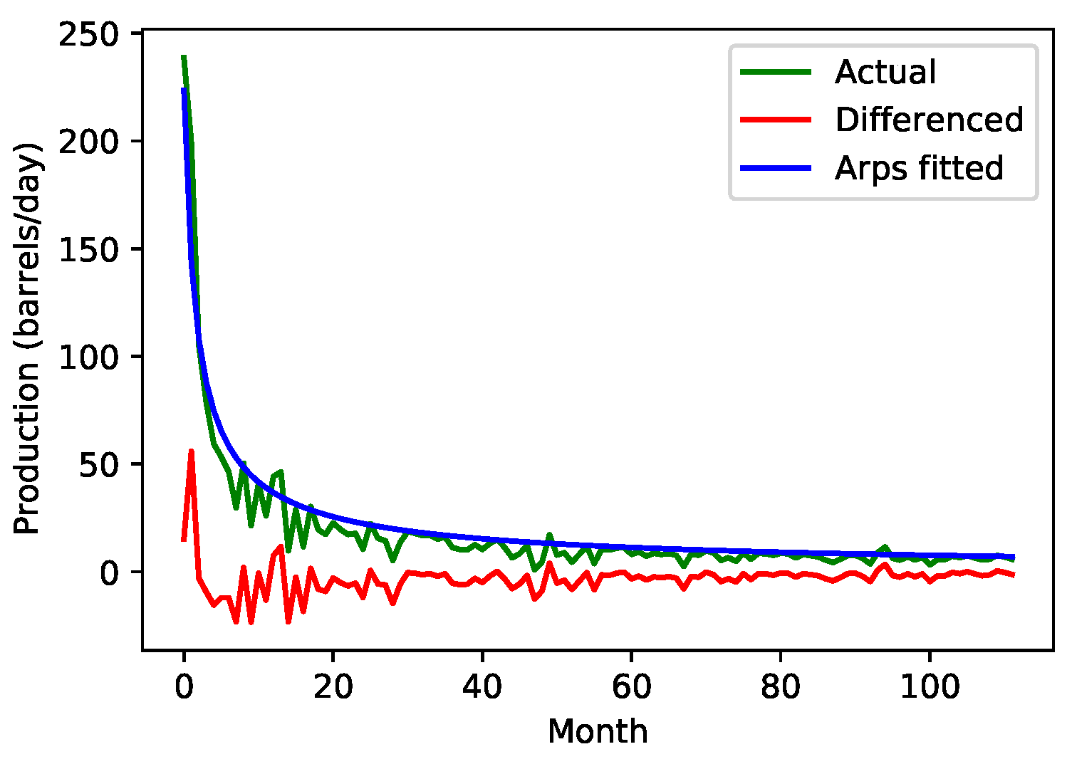
2. Model
3. Data
4. Evaluation Metrics
5. Results and Discussion
6. Conclusions and Future Work
Author Contributions
Funding
Data Availability Statement
Conflicts of Interest
References
- Zeng, Y.-R.; Zeng, Y.; Choi, B.; Wang, L. Multifactor-influenced energy consumption forecasting using enhanced back-propagation neural network. Energy 2017, 127, 381–396. [Google Scholar] [CrossRef]
- Khosravi, A.; Nahavandi, S.; Creighton, D. Quantifying uncertainties of neural network-based electricity price forecasts. Appl. Energy 2013, 112, 120–129. [Google Scholar] [CrossRef]
- Soman, S.S.; Zareipour, H.; Malik, O.; Mandal, P. A review of wind power and wind speed forecasting methods with different time horizons. In Proceedings of the North American Power Symposium 2010, Arlington, TX, USA, 26–28 September 2010; pp. 1–8. [Google Scholar]
- Romeu, P.; Zamora-martínezz, F.; Botella-Rocamora, P.; Pardo, J. Time-series forecasting of indoor temperature using pre-trained deep neural networks. In Proceedings of the International Conference on Artificial Neural Networks; Springer: Berlin/Heidelberg, Germany, 2013; pp. 451–458. [Google Scholar]
- Gooijer, J.G.D.; Hyndman, R.J. 25 years of time series forecasting. Int. J. Forecast. 2006, 22, 443–473. [Google Scholar] [CrossRef]
- Wang, H.; Yi, H.; Peng, J.; Wang, G.; Liu, Y.; Jiang, H.; Liu, W. Deterministic and probabilistic forecasting of photovoltaic power base don deep convolutional neural network. Energy Convers. Manag. 2017, 153, 409–422. [Google Scholar] [CrossRef]
- Camporeale, E.; Chu, X.; Agapitov, O.; Bortnik, J. On the generation of probabilistic forecasts from deterministic models. Space Weather 2019, 17, 455–475. [Google Scholar] [CrossRef]
- Kirchgässner, G.; Wolters, J.; Hassler, U. Introduction to Modern Time Series Analysis; Springer Science & Business Media: Berlin/Heidelberg, Germany, 2012. [Google Scholar]
- Chang, F.; Huang, H.; Chan, A.H.; Man, S.S.; Gong, Y.; Zhou, H. Capturing long-memory properties in road fatality rate series by an autoregressive fractionally integrated moving average model with generalized autoregressive conditional heteroscedasticity: A case study of florida, the united states, 1975–2018. J. Saf. Res. 2022, 81, 216–224. [Google Scholar] [CrossRef] [PubMed]
- Nason, G.P. Stationary and non-stationary time series. In Statistics in Volcanology; Geological Society of London: London, UK, 2006; Volume 60. [Google Scholar]
- Cecaj, A.; Lippi, M.; Mamei, M.; Zambonelli, F. Comparing deep learning and statistical methods in forecasting crowd distribution from aggregated mobile phone data. Appl. Sci. 2020, 10, 6580. [Google Scholar] [CrossRef]
- Bahdanau, D.; Cho, K.; Bengio, Y. Neural machine translation by jointly learning to align and translate. arXiv 2014, arXiv:1409.0473. [Google Scholar]
- Zhang, Y.-J.; Chen, M.-Y. Evaluating the dynamic performance of energy portfolios: Empirical evidence from the dea directional distance function. Eur. J. Oper. Res. 2018, 269, 64–78. [Google Scholar] [CrossRef]
- Ma, X.; Liu, Z. Predicting the oil production using the novel multivariate nonlinear model based on arps decline model and kernel method. Neural Comput. Appl. 2018, 29, 579–591. [Google Scholar] [CrossRef]
- Manda, P.; Nkazi, D.B. The evaluation and sensitivity of decline curve modelling. Energies 2020, 13, 2765. [Google Scholar] [CrossRef]
- Afifi, H.; Elmahdy, M.; Saban, M.E.; Abu-Elkheir, M. Probabilistic time series forecasting for unconventional oil and gas producing wells. In Proceedings of the 2020 2nd Novel Intelligent and Leading Emerging Sciences Conference (NILES), Giza, Egypt, 24–26 October 2020; pp. 450–455. [Google Scholar]
- The Base Layer Class. Available online: https://keras.io/api/layers/baselayer/layer-class (accessed on 30 May 2021).
- der Meer, D.W.V.; Widén, J.; Munkhammar, J. Review on probabilistic forecasting of photovoltaic power production and electricity consumption. Renew. Sustain. Energy Rev. 2018, 81, 1484–1512. [Google Scholar] [CrossRef]
- Khosravi, A.; Nahavandi, S.; Creighton, D.; Atiya, A.F. Lower upper bound estimation method for construction of neural network-based prediction intervals. IEEE Trans. Neural Netw. 2010, 22, 337–346. [Google Scholar] [CrossRef] [PubMed]
- Petneházi, G. Recurrent neural networks for time series forecasting. arXiv 2019, arXiv:1901.00069. [Google Scholar]

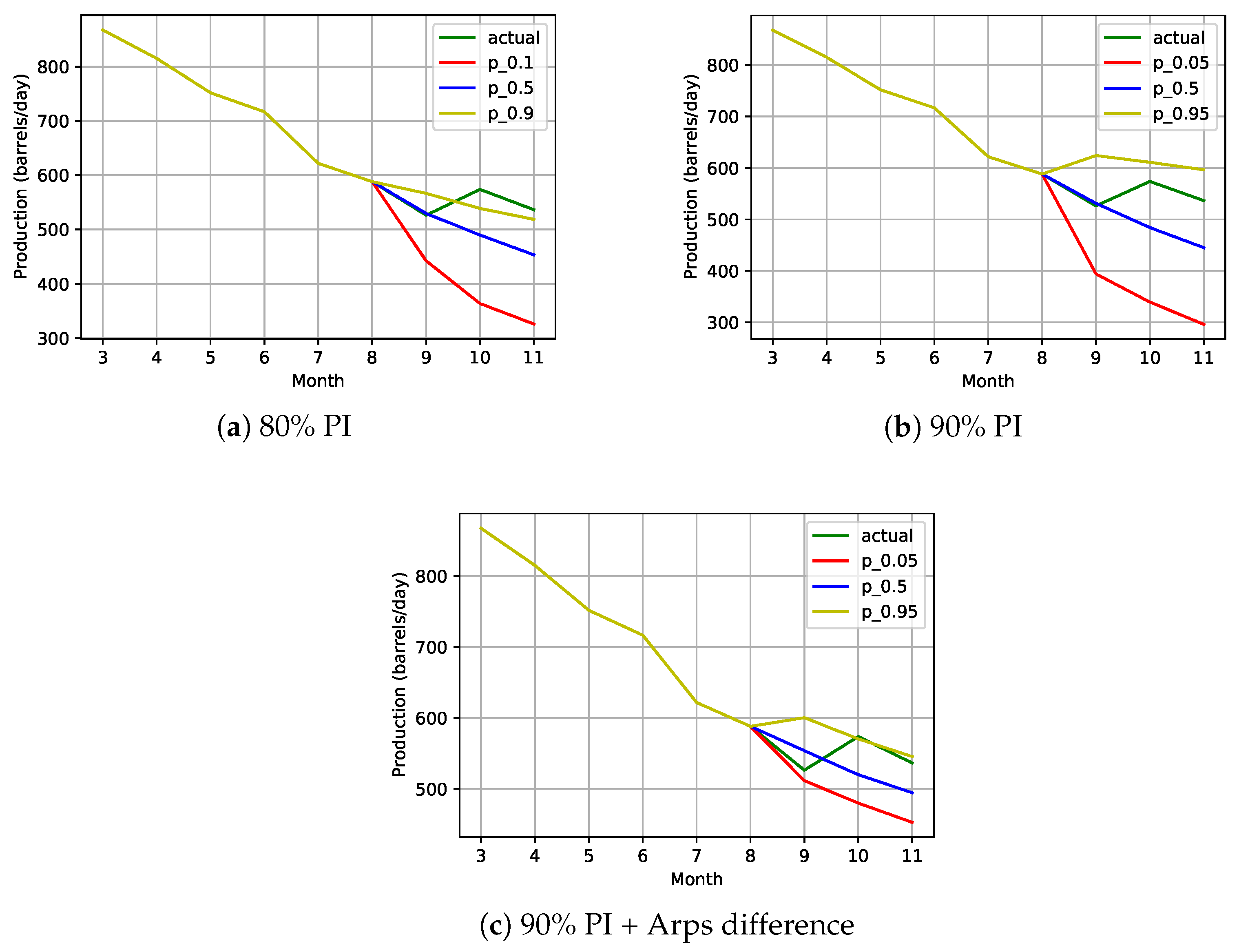
| Set-Up | PICP | PINAW | CWC η = 50 |
|---|---|---|---|
| 90 PI + Arps | 85.9 | 6.9 | 60.5 |
| 90 PI + Attention | 90.49 | 9.4 | 9.4 |
| 90 PI + Arps + Attention | 85.42 | 6.7 | 72.9 |
| 90 PI | 90.93 | 9.8 | 9.8 |
| 80 PI | 82.16 | 6.4 | 6.4 |
| Set-Up | Step 1 | Step 2 | Step 3 | Aggregation | ||||
|---|---|---|---|---|---|---|---|---|
| PICP | PINAW | PICP | PINAW | PICP | PINAW | PICP | PINAW | |
| Direct 80 | 82.4 | 4.7 | 81.4 | 6.6 | 81.0 | 8.0 | 81.64 | 5.2 |
| Direct 90 | 91.1 | 7.9 | 90.7 | 11.0 | 90.6 | 12.9 | 90.80 | 8.6 |
| Arps Difference Direct 90 | 86.6 | 6.1 | 85.1 | 8.3 | 84.1 | 9.7 | 85.23 | 6.5 |
Publisher’s Note: MDPI stays neutral with regard to jurisdictional claims in published maps and institutional affiliations. |
© 2022 by the authors. Licensee MDPI, Basel, Switzerland. This article is an open access article distributed under the terms and conditions of the Creative Commons Attribution (CC BY) license (https://creativecommons.org/licenses/by/4.0/).
Share and Cite
Afifi, H.; Elmahdy, M.; El Saban, M.; Abu-Elkheir, M. Probabilistic Forecasting for Oil Producing Wells Using Seq2seq Augmented Model. Eng. Proc. 2022, 18, 16. https://doi.org/10.3390/engproc2022018016
Afifi H, Elmahdy M, El Saban M, Abu-Elkheir M. Probabilistic Forecasting for Oil Producing Wells Using Seq2seq Augmented Model. Engineering Proceedings. 2022; 18(1):16. https://doi.org/10.3390/engproc2022018016
Chicago/Turabian StyleAfifi, Hadeel, Mohamed Elmahdy, Motaz El Saban, and Mervat Abu-Elkheir. 2022. "Probabilistic Forecasting for Oil Producing Wells Using Seq2seq Augmented Model" Engineering Proceedings 18, no. 1: 16. https://doi.org/10.3390/engproc2022018016
APA StyleAfifi, H., Elmahdy, M., El Saban, M., & Abu-Elkheir, M. (2022). Probabilistic Forecasting for Oil Producing Wells Using Seq2seq Augmented Model. Engineering Proceedings, 18(1), 16. https://doi.org/10.3390/engproc2022018016