Backstepping Control of Drone ^†

Abstract

This work derives the models which can be used to design and implement control laws for six degrees-of-freedom (DOF) quadrotor stability. The first part of this paper deals with the presentation of the background of quadrotor modeling; the second part describes the direct control of the drone using the backstepping control principal. This principal is based on the division of the system into several sub-systems in a cascade, which makes the control laws generated on each subsystem, in a decreasing manner, until a global control law for the whole system is generated. The simulation results for the sm controller are generated on the MATLAB/Simulink platform; the results show a good performance in both the transient and steady-state operations.

1. Introduction

Drones are used as a means of monitoring and following important events such as forest fires and political demonstrations; they can also be used to rescue people in earthquakes in the civilian field. Additionally, they can be used as tools for supervision and fault diagnostic in smart grid systems. Drones can also act as aerial base stations (BSs) to deliver communication services (both uplink and downlink) for the subscribers on the ground [1]. In the military field, drones reduce human losses and material; they are able to closely monitor the enemy and reveal their location without exposing individuals to danger, and can direct precise strikes, like helicopters and aircrafts.

Many control approaches were developed for unmanned aerial vehicles (UAVS) in the literature. Hence, a detailed drone description model is described in [2,3,4]. The sliding mode control strategy based on backstepping control is widely used as it can produce high performances and a faster response for drone systems in general [5,6,7,8,9] and in indoor micro-quadrotors in particular [10]. Modeling- and backstepping-based nonlinear control for a six-DOF quadrotor helicopter is proposed by [11], in addition to the proposition of an adaptive sliding mode control for a quadrotor helicopter in [12].

Quadrotor mathematical modeling is very complicated [13]. It presents non-linearity due to having six degrees of freedom (translational and rotational motion) with only four control inputs. To preserve the equilibrium or the desired attitude of the drone, a traditional PID controller is commonly used; however, it does not ensure the robustness of the quadrotor, whatever the controlling target Euler angle or angular rate is. Hence, new approaches have proposed the use of a cascade PID algorithm to provide better performance and motion stabilization [14,15]. However, the implemented system still needs to tackle the drone system’s non-linearity.

Hence, to control such a system, a backstepping method is the best choice [16,17]. Backstepping control is based on the Lyapunov stability principle of dynamic systems, and it is robust to parametric variation; thus, it ensures the stability of the system and gives good performances results.

This work describes the direct control of the drone using the backstepping control principal, where the quadrotor is supposed to track the desired trajectories with an acceptable dynamic. This paper is treated in three mean parts, organized as follows: first, the mathematical model of the quadrotor is developed; in the second step, the algorithm of backstepping control is presented; in the last section, the simulation results and their interpretations are presented. Finally, the conclusion and possible future developments of the work are presented.

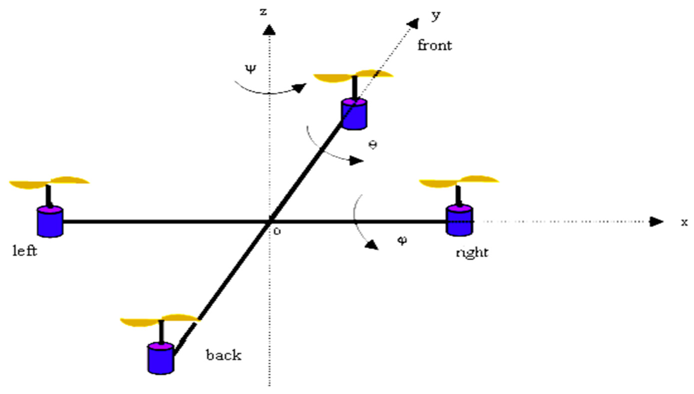
2. Quadrotor Dynamic Modeling

The quadrotor consists of four rotors in a cross-configuration, as shown in Figure 1. The four-rotor design allows the quadrotor to be relatively simple in design yet highly reliable and maneuverable. The dynamic equation of movement of the attitude could be deduced from the Euler equation. The quadrotor mathematical and state-space models are explained in the following subsections.

2.1. Drone Dynamic Model

The dynamic model of the quadrotor can be defined in terms of the position vector and force expressions as given in Equations (1)–(3).

$$\{\begin{array}{l}{x}^{"}=-\frac{T}{m}[\sin (\phi )\sin (\psi )+\cos (\phi )\cos (\theta )\cos (\psi )]\\ \hspace{0.17em}{y}^{"}=-\frac{T}{m}[\cos (\phi )\sin (\theta )\sin (\psi ) - \sin (\psi \left)\cos \right(\theta \left)\right]\hspace{1em}\\ z^{"}=g-\frac{T}{m}[\cos (\phi )\cos (\theta )]\hspace{1em}\hspace{1em}\hspace{1em}\hspace{1em}\hspace{1em}\hspace{1em}\hspace{1em}\hspace{0.17em}\hspace{1em}\end{array}$$

(1)

Such that (x”, y”, z”) represents the second derivative of position vector, $T$ is the torque, and $m$ denotes the mass of the drone.

The moment equations can be expressed in terms of the orientation angles $\left(\phi ,\theta ,\psi \right)$ —roll, pitch, and yaw, respectively—as given in Equations (2) and (3).

$$\{\begin{array}{l}{p}^{’}=\frac{I_z{-I}_y}{I_x}qr-\frac{J_r}{I_x}\mathsf{\Omega }q+\frac{1}{I_x}{\tau }_{\varphi }\\ q^{’}=\frac{I_z{-I}_x}{I_y}pr-\frac{J_r}{I_y}\mathsf{\Omega }p+\frac{1}{I_y}{\tau }_{\theta }\\ r^{’}=\frac{I_y{-I}_x}{I_z}pq+\frac{1}{I_z}{\tau }_{\psi }\hspace{1em}\hspace{1em}\hspace{1em}\end{array}$$

(2)

$$\{\begin{array}{l}{\phi }^{’}=p+q\sin (\phi )tg(\theta )+r\cos (\phi )tg(\theta )\\ {\theta }^{’}=q\cos (\phi )-\mathrm{rsin}(\phi )\hspace{1em}\hspace{1em}\hspace{1em}\hspace{1em}\hspace{1em}\hspace{0.17em}\hspace{1em}\\ {\psi }^{’}=q\frac{\sin (\phi )}{\cos (\theta )}+r\frac{\cos (\phi )}{\cos (\theta )}\hspace{1em}\hspace{0.17em}\hspace{1em}\hspace{1em}\hspace{1em}\end{array}$$

(3)

τ_φ, τ_θ, and τ_ψ represent the total rolling, pitching, and yawing torques, while p, q, and r represent the angular velocities in the body frame.

2.2. State-Space Model

A state-space representation is a mathematical model of a physical system as a set of inputs, outputs, and state variables related by first-order differential equations. “State space” refers to the space whose axes are the state variables. The state of the system can be represented as a vector within that space.

In this work, the state-space model of the quadrotor in the inertial frame is developed. Thus, the dynamic model of the quadrotor in the inertial frame can be expressed by the system referred to as Equation (4):

$$\{\begin{array}{l}{x}_1^{’}=x_2\\ x_2^{’}=a_1{x}_4{x}_6+a_3\mathsf{\Omega }{x}_4+b_1{U}_2\hspace{1em}\hspace{1em}\hspace{1em}\hspace{1em}\hspace{1em}\\ x_3^{’}=x_4\hspace{1em}\hspace{1em}\hspace{1em}\hspace{1em}\hspace{1em}\hspace{1em}\hspace{1em}\hspace{1em}\hspace{1em}\hspace{1em}\hspace{1em}\\ x_4^{’}=a_4{x}_2{x}_6+a_6\mathsf{\Omega }{x}_2+b_2{U}_3\hspace{1em}\hspace{1em}\hspace{1em}\hspace{1em}\\ x_5^{’}=x_6\hspace{1em}\hspace{1em}\hspace{1em}\hspace{1em}\hspace{1em}\hspace{1em}\hspace{1em}\hspace{1em}\hspace{1em}\hspace{1em}\hspace{1em}\\ x_6^{’}=a_7{x}_2{x}_4+b_3{U}_4\hspace{1em}\hspace{1em}\hspace{1em}\hspace{1em}\hspace{0.17em}\hspace{1em}\hspace{1em}\hspace{0.17em}\hspace{0.17em}\hspace{0.17em}\\ x_7^{’}=x_8\hspace{1em}\hspace{1em}\hspace{1em}\hspace{1em}\hspace{1em}\hspace{1em}\hspace{1em}\hspace{1em}\hspace{1em}\hspace{1em}\hspace{1em}\\ x_8^{’}=\frac{\cos (x_1)\cos (x_2)}{m}{U}_1-g\hspace{1em}\hspace{1em}\hspace{1em}\hspace{1em}\hspace{1em}\\ x_9^{’}=x_{10}\hspace{1em}\hspace{1em}\hspace{1em}\hspace{1em}\hspace{1em}\hspace{1em}\hspace{1em}\hspace{1em}\hspace{1em}\hspace{1em}\hspace{1em}\\ x_{10}^{’}=U_y\frac{U_1}{m}\hspace{1em}\hspace{1em}\hspace{1em}\hspace{1em}\hspace{1em}\hspace{1em}\hspace{1em}\hspace{1em}\hspace{1em}\hspace{1em}\hspace{0.17em}\\ x_{11}^{’}=x_{12}\hspace{1em}\hspace{1em}\hspace{1em}\hspace{1em}\hspace{1em}\hspace{1em}\hspace{1em}\hspace{1em}\hspace{1em}\hspace{1em}\hspace{1em}\\ x_{12}^{’}=U_x\frac{U_1}{m}\hspace{1em}\hspace{1em}\hspace{1em}\hspace{1em}\hspace{1em}\hspace{1em}\hspace{1em}\hspace{0.17em}\hspace{0.17em}\hspace{1em}\hspace{1em}\hspace{1em}\hspace{0.17em}\end{array}$$

(4)

The parameters a₁, a₄, a₇, b₁, b₂, and b₃ can be calculated as follows:

$$\begin{array}{l}{a}_1=\frac{I_y{-I}_z}{I_x}, a_3=\frac{J_r}{I_x}, a_4=\frac{I_z{-I}_x}{I_y}, a_6=\frac{J_r}{I_y}, a_7=\frac{I_x{-I}_y}{I_z},\\ b_1=\frac{d}{I_x}, b_2=\frac{d}{I_y}, b_3=\frac{d}{I_z}\end{array}$$

I_x, I_y, and I_z denote the inertias of the x-, y-, and z-axis of the quadrotor, respectively; J_r denotes the z-axis inertia of the propellers’ rotors.

$$\begin{array}{ll}\mathrm{whereas}& U_x=\cos (x_1)\cos (x_3)\cos (x_5)+\sin (x_1)\sin (x_5)\\ & U_y=\cos (x_1)\sin (x_3)\sin (x_5)-\sin (x_1)\cos (x_5)\end{array}$$

To solve the given system, a backstepping control scheme is used as detailed in the following section.

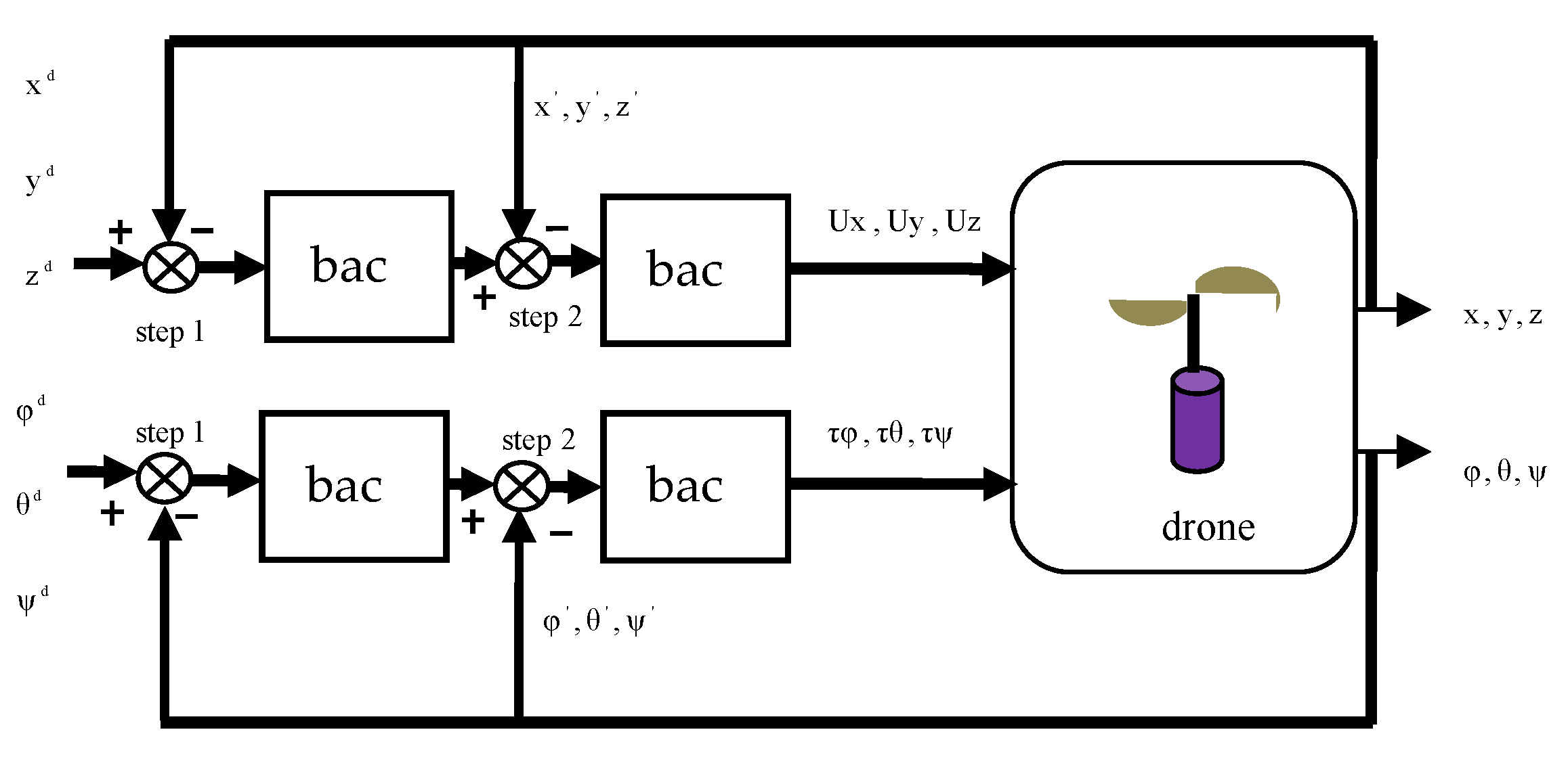
3. Backstepping Control of Drone

The principle of backstepping is to divide the system into several sub-systems in a cascade. The control laws are then made for each subsystem, in a decreasing manner, until a global control law for the whole system is generated.

3.1. Control of the Angle φ

Considering the first subsystem mentioned below:

$$\{\begin{array}{l}{x}_1^{’}=x_2\hspace{1em}\hspace{1em}\hspace{1em}\hspace{1em}\hspace{1em}\hspace{1em}\hspace{1em}\hspace{1em}\\ x_2^{’}=x_4{x}_6{a}_1{-x}_4\mathsf{\Omega }{a}_2+b_1{U}_2\end{array}$$

(5)

step1

The error ${\epsilon }_1$ between the desired and actual roll angle is expressed as follows: ${\epsilon }_1=x_1^d-x_1$. Consider the Lyapunov function $V_1=\frac{1}{2}{\epsilon }_1^2$, where the derivate of V₁ along x₁ trajectory, V’, is computed as follows:

$$V_1^{’}={\epsilon }_1{\epsilon }_1^{’} \mathrm{with}: {\epsilon }_1^{’}=x_1^{d’}{-x}_1^{’}=x_1^{d’}{-x}_2$$

Choosing $\epsilon {’}_1={-K}_1{\epsilon }_1$ (knowing that: $K_1{\epsilon }_1$ is positive definite function). Thus, the desired $x_2^d$ is extracted as: $x_2^d=x_1^{d’}+K_1{\epsilon }_1$

step2

Denoting ${\epsilon }_2$ the error between desired and actual roll angle rate, so that: ${\epsilon }_2=x_2^d-x_2$. Using $V_2=V_1+\frac{1}{2}{\epsilon }_2^2$ as a candidate Lyapunov function, we obtain:

$$\begin{array}{l}{V}_2^{’}=V_1^{’}+{\epsilon }_2{\epsilon }_2^{’}={\epsilon }_1{\epsilon }_1^{’}+{\epsilon }_2{\epsilon }_2^{’}={\epsilon }_2\left(x_1^{d’}{-x}_2\right)+{\epsilon }_2(x_2^d{-x}_2^{’})\\ ={\epsilon }_1(x_1^d{-(x}_2^{d’}-{\epsilon }_2))+{\epsilon }_2(x_2^d{-(x}_4{x}_6{a}_1{-x}_4\mathsf{\Omega }{a}_2+b_{1}U))\\ ={\epsilon }_1(x_1^d{-x}_2^{d’})+{\epsilon }_1{\epsilon }_2+{\epsilon }_2(x_2^{d’}{-(x}_4{x}_6{a}_1{-x}_4\mathsf{\Omega }{a}_2+b_{1}U))\\ =-K_1{\epsilon }_1^2+{\epsilon }_2({\epsilon }_1+x_2^d{-x}_4{x}_6{a}_1+x_4\mathsf{\Omega }{a}_2{-b}_{1}U)\\ {\epsilon }_1+x_2^{d’}{-x}_4{x}_6{a}_1+x_4\mathsf{\Omega }{a}_2{-b}_{1}U={-K}_2{\epsilon }_2\end{array}$$

where K₂ is a positive constant and $x_2^{d’}={\alpha }_1^{’}=\left[K_1\left(x_1^d{-x}_1\right)+x_1^{d’}\right]={-K}_1\left(x_2\right)$.

Thus, the control law is expressed by: $U_2=\frac{1}{b}\left[{\epsilon }_1{-K}_1{x}_2{-x}_4{x}_6{a}_1+x_4\mathsf{\Omega }{a}_2+K_2{\epsilon }_2\right]$

3.2. Control of the Angle $\theta$

Considering the second subsystem mentioned below:

$$\{\begin{array}{l}{x}_3^{’}=x_4\hspace{1em}\hspace{1em}\hspace{1em}\hspace{1em}\hspace{1em}\hspace{1em}\hspace{1em}\hspace{1em}\\ x_4^{’}=x_2{x}_6{a}_4+x_2\mathsf{\Omega }{a}_6+b_2{U}_3\end{array}$$

(6)

step1

Considering ${\epsilon }_3$ is the error between the desired and actual angle $\theta$ and can be found by:

$${\epsilon }_3=x_3^d{-x}_3\Rightarrow {\epsilon }_3^{’}=x_3^{d’}{-x}_3^{’}$$

using Lyapunov stability by choosing: $V({\epsilon }_3)=\frac{1}{2}{\epsilon }_3^2$. Therefore, if V’ is negative, then the system trajectory is ensured to verify this condition:

$$v^{’}(\epsilon )={\epsilon }_3{\epsilon }_3^{’}={\epsilon }_3(x_3^{d’}{-x}_4)<0, \mathrm{then}: x_3^{d’}{-x}_4=-{{\rm K}}_3{\epsilon }_3\Rightarrow x_4^d=x_3^{d’}+K_3{\epsilon }_3$$

step2

The error ${\epsilon }_4=x_4^d{-x}_4\Rightarrow x_4=x_4^d-{\epsilon }_4$$\Rightarrow$${\epsilon }_4^{’}=x_4^{d’}{-x}_4^{’}$

$$\begin{array}{l}{V}_4=V_3+\frac{1}{2}{\epsilon }_4^2\Rightarrow V_4^{’}={\epsilon }_3{\epsilon }_3^{’}+{\epsilon }_4{\epsilon }_4^{’}\\ {\epsilon }_3^{’}=x_3^{d’}{-x}_4^d+{\epsilon }_4\Rightarrow {\epsilon }_3{\epsilon }_3^{’}={\epsilon }_3(x_3^{d’}{-x}_4^d+{\epsilon }_4)+{\epsilon }_4\left({\epsilon }_4^{’}\right)\\ {\epsilon }_3{\epsilon }_3^{’}={\epsilon }_3\left(x_3^{d’}{-x}_4^d\right)+{\epsilon }_3{\epsilon }_4+{\epsilon }_4\left({\epsilon }_4^{’}\right)={\epsilon }_4({\epsilon }_3+x_4^{d’}{-(a}_3{x}_2{x}_6+a_4\mathsf{\Omega }{x}_2+b_2{U}_3\left)\right)\\ {\epsilon }_3+x_4^{d’}{-a}_3{x}_2{x}_6{-a}_4\mathsf{\Omega }{x}_2{-b}_2{U}_3={-K}_4{\epsilon }_4\\ b_2{U}_3={\epsilon }_3+x_4^{d’}{-a}_3{x}_2{x}_6{-a}_4\mathsf{\Omega }{x}_2+K_4{\epsilon }_4\\ U_3=\frac{1}{b_2}\left[{\epsilon }_3{-a}_3{x}_2{x}_6{-a}_4\mathsf{\Omega }{x}_2+K_4{\epsilon }_4{-K}_3{x}_4\right]\end{array}$$

3.3. Control of the Angle $\psi$

Now, consider the third subsystem mentioned below:

$$\{\begin{array}{l}{x}_5^{’}=x_6\hspace{1em}\hspace{1em}\hspace{1em}\hspace{1em}\hspace{1em}\hspace{1em}\hspace{1em}\hspace{1em}\\ x_6^{’}=a_7{x}_2{x}_4+b_3{U}_4\hspace{1em}\hspace{1em}\hspace{1em}\end{array}$$

(7)

step1

Let us name ${\epsilon }_5$ the error between the desired and actual angle $\psi$. Thus:

$${\epsilon }_5=x_5^d{-x}_5\Rightarrow {\epsilon }_5^{’}=x_5^{d’}{-x}_5^{’}$$

With Lyapunov function being $V({\epsilon }_5)=\frac{1}{2}{\epsilon }_5^2$, such that $v^{’}(\epsilon )={\epsilon }_5{\epsilon }_5^{’}={\epsilon }_5(x_5^{d’}{-x}_5)<0$

Thus, $x_5^{d’}{-x}_5^{’}=-K_5{\epsilon }_5^{}$$\Rightarrow$$x_6^d=x_5^{d’}+K_5{\epsilon }_5^{}$

step2

The error ${\epsilon }_6=x_6^d{-x}_{6 }\Rightarrow x_6=x_6^d-{\epsilon }_{6 }{{\displaystyle }}_{}\Rightarrow \epsilon {’}_6=x_6^{d’}-x_6^{’}$

$$\begin{array}{l}{V}_6=V_5+\frac{1}{2}{\epsilon }_6^2\Rightarrow V_6^{’}={\epsilon }_5{\epsilon }_5^{’}+{\epsilon }_6{\epsilon }_6^{’}\\ {\epsilon }_5^{’}=x_5^{d’}{-x}_6^d+{\epsilon }_6\Rightarrow V_6^{’}={\epsilon }_5(x_5^{d’}{-x}_6^d+{\epsilon }_6)+{\epsilon }_6\left({\epsilon }_6^{’}\right)\\ ={\epsilon }_5\left(x_5^{d’}{-x}_6^d\right)+{\epsilon }_5{\epsilon }_6+{\epsilon }_6\left({\epsilon }_6^{’}\right)\\ \Rightarrow {\epsilon }_5+x_6^{d’}{-a}_5{x}_2{x}_4{-b}_3{U}_4={-K}_6{\epsilon }_6\\ ={\epsilon }_6({\epsilon }_5+x_6^{d’}{-(a}_5{x}_2{x}_4+b_3{U}_4\left)\right)\\ b_3{U}_4={\epsilon }_5+x_6^{d’}{-a}_5{x}_2{x}_4+K_6{\epsilon }_6\Rightarrow U_4=\frac{1}{b_3}\left[{\epsilon }_5{-a}_5{x}_2{x}_4{-K}_6{\epsilon }_6{-K}_5{x}_6\right]\end{array}$$

3.4. Control of the Position z

Equation (8) represents the fourth subsystem:

$$\{\begin{array}{l}{x}_7^{’}=x_8\hspace{1em}\hspace{1em}\hspace{1em}\hspace{1em}\hspace{1em}\hspace{1em}\hspace{1em}\hspace{1em}\hspace{1em}\hspace{1em}\hspace{1em}\\ x_8^{’}=\frac{\cos (x_1)\cos (x_2)}{m}{U}_1-g\hspace{1em}\hspace{1em}\end{array}$$

(8)

step1

${\epsilon }_7$ is the error between the desired and actual position z, such that:

$${\epsilon }_7=x_7^d{-x}_7 ; \mathrm{thus},$$

The Lyapunov function is $V({\epsilon }_7)=\frac{1}{2}{\epsilon }_7^2$$\Rightarrow$$v^{’}(\epsilon )={\epsilon }_7{\epsilon }_7^{’}={\epsilon }_7(x_7^{d’}{-x}_8)<0$ Then, $x_7^{d’}{-x}_8=-{{\rm K}}_7{\epsilon }_7\Rightarrow x_8^d=x_7^{d’}+K_7{\epsilon }_7$

step2

The error ${\epsilon }_8=x_8^d{-x}_8\Rightarrow x_8=x_8^d-{\epsilon }_8$ thus, ${\epsilon }_8^{’}=x_8^{d’}{-x}_8^{’}$

$$\begin{array}{l}{V}_8=V_7+\frac{1}{2}{\epsilon }_8^2\Rightarrow V_8^{’}={\epsilon }_7{\epsilon }_7^{’}+{\epsilon }_8{\epsilon }_8^{’}\\ {\epsilon }_7^{’}=x_7^{d’}{-x}_8^d+{\epsilon }_8\Rightarrow {\epsilon }_7{\epsilon }_7^{’}={\epsilon }_7(x_7^{d’}{-x}_8^d+{\epsilon }_8)+{\epsilon }_8\left({\epsilon }_8^{’}\right)\\ {\epsilon }_7{\epsilon }_7^{’}={\epsilon }_7\left(x_7^{d’}{-x}_8^d\right)+{\epsilon }_7{\epsilon }_8+{\epsilon }_8\left({\epsilon }_8^{’}\right)={\epsilon }_8({\epsilon }_7+x_8^{d’}-(g-\frac{U_1}{m}\cos \left(x_1\right)\cos \left(x_3\right))\\ {\epsilon }_7+x_8^{d’}-g+\frac{U_1}{m}\cos \left(x_1\right)\cos \left(x_3\right)={-K}_8{\epsilon }_8\\ \frac{U_1}{m}\cos \left(x_1\right)\cos \left(x_3\right)=-{\epsilon }_7-x_8^{d’}+{g-K}_8{\epsilon }_8\\ U_1=\frac{m}{\cos \left(x_1\right)\cos \left(x_3\right)}\left[-{\epsilon }_7+{g-K}_8{\epsilon }_8{-K}_7{x}_8\right]\end{array}$$

3.5. Control of the Position y

Equation (9) represents the fifth subsystem:

$$\{\begin{array}{l}{x}_9^{’}=x_{10}\hspace{1em}\hspace{1em}\hspace{1em}\hspace{1em}\hspace{1em}\hspace{1em}\hspace{1em}\hspace{1em}\\ x_{10}^{’}=U_y\frac{U_1}{m}\hspace{1em}\hspace{1em}\hspace{1em}\hspace{1em}\hspace{1em}\hspace{1em}\hspace{1em}\end{array}$$

(9)

step1

Name ${\epsilon }_9$ the error between the desired and actual position y

$${\epsilon }_9=x_9^d{-x}_9\Rightarrow {\epsilon }_9^{’}=x_9^{d’}{-x}_9^{’}$$

The Lyapunov function is $V({\epsilon }_9)=\frac{1}{2}{\epsilon }_9^2$$\Rightarrow$$V’(\epsilon )={\epsilon }_9^{}{\epsilon }_9^{’}={\epsilon }_9\left(x_9^{d’}-x_{10}^{}\right)<0$ Then, $x_9^{d’}{-x}_{10}=-{{\rm K}}_9{\epsilon }_9\Rightarrow x_{10}^d=x_9^{d’}+K_9{\epsilon }_9$

step2

The error will be: ${\epsilon }_{10}=x_{10}^d{-x}_{10}\Rightarrow x_{10}=x_{10}^d-{\epsilon }_{10}$$\Rightarrow$${\epsilon }_{10}^{’}=x_{10}^{d’}{-x}_{10}^{’}$

$$\begin{array}{l}{V}_{10}=V_9+\frac{1}{2}{\epsilon }_{10}^2\Rightarrow V^{’}={\epsilon }_9{\epsilon }_9^{’}+{\epsilon }_{10}{\epsilon }_{10}^{’}\\ {\epsilon }_9^{’}=x_9^{d’}{-x}_{10}^d+{\epsilon }_{10}\Rightarrow {\epsilon }_9{\epsilon }_9^{’}={\epsilon }_9(x_9^{d’}{-x}_{10}^d+{\epsilon }_{10})+{\epsilon }_{10}\left({\epsilon }_{10}^{’}\right)\end{array}$$

$$\begin{array}{l}={\epsilon }_9\left(x_9^{d’}{-x}_{10}^d\right)+{\epsilon }_9{\epsilon }_{10}+{\epsilon }_{10}\left({\epsilon }_{10}^{’}\right)={\epsilon }_{10}({\epsilon }_9+x_{10}^{d’}-(-\frac{U_1}{m}{U}_y)\\ {\epsilon }_9+x_{10}^{d’}+\frac{U_1}{m}{U}_y={-K}_{10}{\epsilon }_{\begin{array}{l}10\\ \end{array}}\Rightarrow \frac{U_1}{m}{U}_y=-{\epsilon }_9-x_{10}^{d’}{-K}_{10}{\epsilon }_{10}\\ U_y=\frac{m}{U_1}\left[-{\epsilon }_9{-K}_{10}{\epsilon }_{10}{-K}_9{x}_{10}\right]\end{array}$$

3.6. Control of the Position x

The last subsystem is represented by Equation (10) below:

$$\{\begin{array}{l}{x}_{11}^{’}=x_{12}\hspace{1em}\hspace{1em}\hspace{1em}\hspace{1em}\hspace{1em}\hspace{1em}\hspace{1em}\hspace{1em}\\ x_{12}^{’}=U_x\frac{U_1}{m}\hspace{1em}\hspace{1em}\hspace{1em}\hspace{1em}\hspace{1em}\hspace{1em}\hspace{1em}\end{array}$$

(10)

step1

Name ${\epsilon }_{11}$ the error between the desired and actual position x, such that

$${\epsilon }_{11}=x_{11}^d{-x}_{11}\Rightarrow {\epsilon }_{11}^{’}=x_{11}^{d’}{-x}_{11}^{’}$$

(11)

The Lyapunov function is $V({\epsilon }_{11})=\frac{1}{2}{\epsilon }_{11}^2$$\Rightarrow$ $v^{’}(\epsilon )={\epsilon }_{11}{\epsilon }_{11}^{’}={\epsilon }_{11}(x_{11}^{d’}{-x}_{12})<0$

Thus, $x_{11}^{d’}{-x}_{12}=-{{\rm K}}_{11}{\epsilon }_{11}\Rightarrow x_{12}^d=x_{11}^{d’}+K_{11}{\epsilon }_{11}$

step2

The error is defined by: ${\epsilon }_{12}=x_{12}^d{-x}_{12}\Rightarrow x_{12}=x_{12}^d-{\epsilon }_{12}$ its derivative is ${\epsilon }_{12}^{’}=x_{12}^{d’}{-x}_{12}^{’}$

$$\begin{array}{l}{V}_{12}=V_{11}+\frac{1}{2}{\epsilon }_{12}^2\Rightarrow V^{’}={\epsilon }_{11}{\epsilon }_{11}^{’}+{\epsilon }_{12}{\epsilon }_{12}^{’}\\ {\epsilon }_{11}^{’}=x_{11}^{d’}-x_{12}^d+{\epsilon }_{12}\Rightarrow {\epsilon }_{11}{\epsilon }_{11}^{’}={\epsilon }_{11}(x_{11}^{d’}-x_{12}^d+{\epsilon }_{12})+{\epsilon }_{12}{\epsilon }_{12}^{’}\\ {\epsilon }_{11}+x_{12}^{d’}+\frac{U_1}{m}{U}_x=-K_{12}{\epsilon }_{\begin{array}{l}12\\ \end{array}}\\ \frac{U_1}{m}{U}_x=-{\epsilon }_{11}-x_{11}^{d’}-K_{12}{\epsilon }_{12}\\ U_x=\frac{m}{U_1}\left[-{\epsilon }_{11}{-K}_{12}{\epsilon }_{12}{-K}_{11}{x}_{12}\right]\end{array}$$

All the previous steps of the backstepping control, used to generate a global control law for the whole system, are summarized in the block diagram shown in Figure 2.

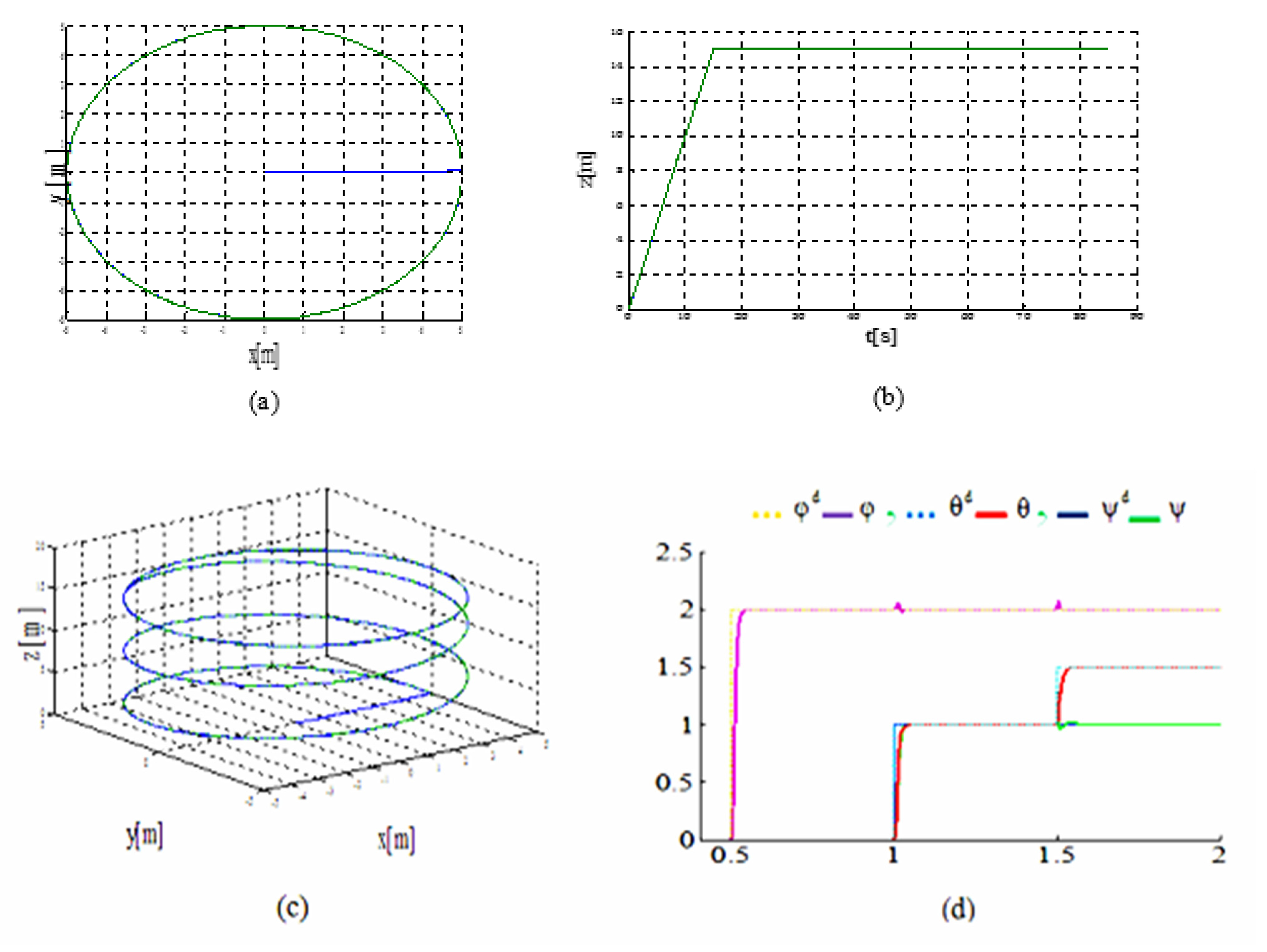
4. Results and Discussions

In order to validate our proposed control solution, the model is simulated under Matlab Simulink software. For that purpose, the results are obtained based on the application of the real parameters summarized on

Table 1. Quadrotor parameter used in our simulation [2].

Gravitational Acceleration	g	9.8 m/s2
Mass of quadrotor	m	0.4794 Kg
Length of wings	l	0.225 m
Rotational inertia	Jx Jy Jz	0.0086 Kg m2 0.0086 Kg m2 0.0172 Kg m2
Residual inertia	Jr	3.740 × 10−5 Kg m2

[2].

In this scenario, it is desired to follow a circular trajectory on the XY plane, centered in the origin. The height z increases uniformly from zero to 15 m (as shown in Figure 3b), where the drone stabilizes.

Figure 3a shows the response of the drone controller to the xy desired value; where we see that the estimated value follows the set-point perfectly. Figure 3c illustrates that the real and the desired positions exactly meet each other in three-dimensional space.

Figure 3d illustrates the response of orientation angles (roll, pitch, and yaw), where the dotted lines denote the desired values and continues-lines shows the estimated values. It is clearly demonstrated that the estimated values track the desired trajectories with an acceptable dynamic.

5. Conclusions

In this paper, a backstepping control is used to provide the dynamic control of the quadrotor. The models derived in this paper are used to design and implement control laws for six-DOF quadrotor stability. For this purpose, firstly, the mathematical model of the quadrotor was developed. Secondly, the backstepping control strategy was devised to control the position and orientation of the quadrotor subsystem. Several scenarios were performed to examine the performance of the backstepping strategy, and we noticed that the simulation results showed the effectiveness of the proposed control. For further work, this approach will be implemented on a quadrotor that will be applied for monitoring and fault diagnostic on a multi-agent-based smart grid [18].

References

1. Alsamhi, S.H.; Ma, O.; Ansari, M.S.; Almalki, F.A. Survey on Collaborative Smart Drones and Internet of Things for Improving Smartness of Smart Cities. IEEE Access 2019, 7, 128125–128152. [Google Scholar] [CrossRef]
2. Shahid, F.; Kadri, B.; Jumani, N.A.; Pirwani, Z. Dynamical Modeling and Control of quadrotor. Trans. Mach. Des. 2016, 4, 50–63. [Google Scholar]
3. Tuan, L.L.; Won, S. PID based sliding mode controller design for the micro quadrotor. In Proceedings of the 2013 13th International Conference on Control, Automation and Systems (ICCAS 2013), Gwangju, Korea, 20–23 October 2013; pp. 1860–1865. [Google Scholar] [CrossRef]
4. Erginer, B.; Altug, E. Modeling and PD Control of a Quadrotor VTOL Vehicle. In Proceedings of the 2007 IEEE Intelligent Vehicles Symposium, Istanbul, Turkey, 13–15 June 2007; pp. 894–899. [Google Scholar] [CrossRef]
5. Bouadi, H.; Bouchoucha, M.; Tadjine, M. Sliding Mode Control based on Backstepping Approach for an UAV Type-Quadrotor. World Acad. Sci. Eng. Technol. Int. J. Mech. Mechatron. Eng. 2007, 1, 2. [Google Scholar] [CrossRef]
6. Zahran, S.; Moussa, A.; El-Sheimy, N. Enhanced Drone Navigation in GNSS Denied Environment Using VDM and Hall Effect Sensor. Int. J. Geo Inf. 2019, 8, 169. [Google Scholar] [CrossRef] [Green Version]
7. Labbadi, M.; Cherkaoui, M.; Houm, Y.E.; Guisser, M. Modeling and Robust Integral Sliding Mode Control for a Quadrotor Unmanned Aerial Vehicle. In Proceedings of the 2018 6th International Renewable and Sustainable Energy Conference (IRSEC), Rabat, Morocco, 5–8 December 2018; pp. 1–6. [Google Scholar] [CrossRef]
8. Mohamed, H.A.F.; Yang, S.S.; Moghavvemi, M. Sliding mode controller design for a flying quadrotor with simplified action planner. In Proceedings of the 2009 ICCAS-SICE, Fukuoka, Japan, 18–21 August 2009; pp. 1279–1283. [Google Scholar]
9. Bouadi, H.; Cunha, S.S.; Drouin, A.; Mora-Camino, F. Adaptive sliding mode control for quadrotor attitude stabilization and altitude tracking. In Proceedings of the 2011 IEEE 12th International Symposium on Computational Intelligence and Informatics (CINTI), Budapest, Hungary, 21–22 November 2011; pp. 449–455. [Google Scholar] [CrossRef] [Green Version]
10. Bouabdallah, S.; Siegwart, R. Backstepping and Sliding-mode Techniques Applied to an Indoor Micro Quadrotor. In Proceedings of the 2005 IEEE International Conference on Robotics and Automation, Barcelona, Spain, 18–22 April 2005; pp. 2247–2252. [Google Scholar] [CrossRef] [Green Version]
11. Mian, A.; Daobo, W. Modeling and backstepping-based nonlinear control strategy for a 6 dof quadrotor helicopter. Chin. J. Aeronaut. 2008, 21, 261–268. [Google Scholar] [CrossRef] [Green Version]
12. Lee, D.; Kim, H.J.; Sastry, S. Feedback linearization vs. adaptive sliding mode control for a quadrotor helicopter. Int. J. Control. Autom. Syst. 2009, 7, 419–428. [Google Scholar] [CrossRef]
13. McKerrow, P. Modelling the Draganflyer four-rotor helicopter. In Proceedings of the IEEE International Conference on Robotics and Automation, 2004 Proceedings. ICRA ‘04. 2004, New Orleans, LA, USA, 26 April–1 May 2004; Volume 4, pp. 3596–3601. [Google Scholar] [CrossRef] [Green Version]
14. Hanani, N.; Syazwanadira, F.; Fakharulrazi, N.A.; Yakub, F.; Rasid, Z.A.; Sarip, S. Full Control of Quadrotor Unmanned Aerial Vehicle using Multivariable Proportional Integral Derivative Controller. In Proceedings of the 2019 IEEE 9th International Conference on System Engineering and Technology (ICSET), Shah Alam, Malaysia, 7 October 2019; pp. 447–452. [Google Scholar] [CrossRef]
15. Wang, P.; Man, Z.; Cao, Z.; Zheng, J.; Zhao, Y. Dynamics modelling and linear control of quadcopter. In Proceedings of the 2016 International Conference on Advanced Mechatronic Systems (ICAMechS), Melbourne, VIC, Australia, 30 November–3 December 2016; pp. 498–503. [Google Scholar] [CrossRef]
16. Glida, H.E.; Abdou, L.; Chelihi, A.; Sentouh, C.; Hasseni, S.-E.-I. Optimal model-free backstepping control for a quadrotor helicopter. Nonlinear Dyn. 2020, 100, 3449–3468. [Google Scholar] [CrossRef]
17. Basri, M.A.M.; Noordin, A. Optimal backstepping control of quadrotor UAV using gravitational search optimization algorithm. Bull. Electr. Eng. Inform. 2020, 9, 1819–1826. [Google Scholar] [CrossRef]
18. Hadjira, B.; Rabiai, Z. Decentralized Energy Management System Enhancement for Smart Grid. In Optimizing and Measuring Smart Grid Operation and Control; Recioui, A., Bentarzi, H., Eds.; IGI Global: Hershey, PA, USA, 2021; pp. 156–169. [Google Scholar] [CrossRef]
Figure 1. Quadrotor configuration.
Engproc 14 00004 g001
Figure 2. System block diagram.
Engproc 14 00004 g002
Figure 3. Simulation results. (a) xy drone control. (b) Uniform increase in z height from zero to 15 m. (c) Real and the desired positions exactly meet each other. (d) Orientation angles’ response.
Engproc 14 00004 g003