Aircraft Localization Using ATC Data with Nanosecond Precision from Distributed Crowdsourced Receivers ^†

Abstract

In this paper, we present the first place solution for the Aircraft Localization Competition, which was held on the AIcrowd platform between 15 June 2020 and 31 January 2021 and was organized by the OpenSky Network and the Cyber-Defence Campus of armasuisse Science and Technology. The data for the competition was collected by the OpenSky Network from hundreds of crowdsourced low-cost receivers with nanosecond precision timestamps. Many receivers experienced clock drift and random walk and even provided fully broken timestamps. The solution combines well-known multilateration positioning with a variety of filtering methods and two tailored models for radio wave propagation and receiver clock drift to predict unknown aircraft locations. In this solution, we managed to synchronize 241 receivers, including 36 GPS-equipped, and achieved 81.9 m RMSE 2D distance prediction accuracy on $70\%$ of samples on the private leaderboard.

1. Introduction

Air Traffic Control (ATC) is the key service that enables safety and regulation of airspace for commercial, military and private aircrafts. Its efficiency relies on accurate and robust aircraft localization (i.e., aircraft coordinates at any given moment of time) and quality of prediction of an aircraft’s trajectory in the future. Therefore, it is not surprising that new methods of aircraft localization are constantly being sought.

From the other side, the latest advances in machine learning algorithms have also warmed up interest to new localization methods in recent years. For example, in 2021, the famous platform for data science competitions, Kaggle, in partnership with Microsoft Research and XYZ10, organized a competition to search for the best methods for indoor positioning [1]. It was held between 28 January and 17 May 2021 and challenged participants to track smartphones’ locations by using WiFi, Bluetooth iBeacon, IMU (accelerometer, gyroscope) and geomagnetic field (magnetometer) readings. Other research on indoor positioning proposed mathematical methods to determine the location of a mobile terminal using asynchronous networks of “anchor” nodes in known positions [2].

Going back to aircraft localization, new aircraft surveillance technologies like ADS-B are being developed and deployed worldwide, allowing aircrafts to determine their position via GPS/GNSS and other sensors and broadcast it periodically. ADS-B is considered complementary to traditional radar systems technology, which also requires ground-based stations joined in networks to receive ADS-B information from aircrafts and to track them. In this paper, we will consider ATC networks consisting of crowdsourced, low-cost, ground-based receivers. Such networks are already used by some online services like FlightRadar24 and FlightAware and research networks like OpenSky. The idea to utilize an ensemble of randomly located, low-quality, ground-based receivers to track aircrafts has some strong advantages and challenges. This work is focused on the synchronization of stations having strong clock drift or even providing completely broken timestamps.

The Aircraft Localization competition [3] organized by the OpenSky Network consisted of two rounds and was held between 15 June and 31 July 2020 (round one) and between 1 December 2020 and 31 January 2021 (round two). Participants were challenged to determine unknown positions of aircrafts using time of arrival and signal strength measurements reported by OpenSky Network sensors and barometric altitude measurements reported by aircrafts. In the first round, all data was collected from GPS-equipped sensors, while in the second round, only some sensors were synchronized. The author won fourth place in round one and first place in round two. Methodology and results for the first place solution will be described in the next sections. Here and thereafter, by data and solution, we will mean the round two data and solution.

2. Methodology

The competition dataset consisted of 2629 aircraft tracks with known locations (the training dataset) and 300 aircraft tracks for which $70\%$ or more aircraft locations need to be determined (the test dataset). Training and testing data was collected for the same time interval (1 h) for different aircrafts.

In this solution, aircraft locations were determined using the well-known multilateration technique, which will be described in Section 2.4. After that, predicted locations were filtered, and aircraft tracks were produced where possible. However, to enable aircraft localization, 241 stations were synchronized in advance, and this part of the solution was the most complex one by the author’s opinion. By synchronization, here we mean the correction of stations’ timestamps (using the methodology described in Section 2.2) in order to remove any clock drifts and shifts. In addition, two mathematical models were developed: the radio wave velocity model and the receiver clock drift model, which will be described in Section 2.1 and Section 2.2.

2.1. Radio Wave Velocity Model

The aircraft localization method is based on the estimation of a distance between an aircraft and ground-based stations, which, in turn, are estimated from measurements of time-of-flight of radio signals emitted by an aircraft. Since timestamps in this competition were provided with nanosecond precision, it was very important to develop an accurate model for radio wave velocity in the atmosphere.

Radio wave velocity depends on refractive index of the atmosphere and, therefore, on altitude. It would be a mistake to consider it equal to the speed of light. In round one of the competition, the top three teams used a constant value for radio wave velocity, which was equal to the one at sea level or was estimated together with optimization of ground stations’ locations.

In this paper, dependence of refractive index of the atmosphere on altitude was taken from [4], so radio wave velocity can be written as follows:

$$v\left(h\right)=\frac{c}{n\left(h\right)}=\frac{c}{1+A_0·e^{-B·h}}$$

(1)

where c is the speed of light, h is altitude, $n\left(h\right)$ is refractive index, and $A_0$ and B are some constants.

In this form, radio wave velocity is not suitable for use in multilateral equations because it will require integration over the wave path multiple times. Here we consider effective radio wave velocity instead, which is considered constant along the wave path but depends on altitudes of an aircraft and a ground station:

$$\widehat{v}=const=\frac{L}{\int dt\left(h\right)}$$

(2)

$$\begin{array}{c}\int dt\left(h\right)={\int }_0^L\frac{1+A_0·e^{-B·l·sin\varphi }}{c}·dl={\int }_{h1}^{h2}\frac{1+A_0·e^{-B·h}}{c·sin\varphi }·dh=\hfill \\ \hfill \frac{h_2-h_1}{c·sin\varphi }+\frac{A_0}{c·B·sin\varphi }·\left(e^{-B·h_1}-e^{-B·h_2}\right)\end{array}$$

(3)

where L is a wave path and $h_1$ and $h_2$ are the initial and final altitudes of the wave path. After inserting $L=\frac{h_2-h_1}{sin\varphi }$, effective radio wave velocity has the final form:

$$\widehat{v}=\frac{c}{1+\frac{A_0}{B·\left(h_2-h_1\right)}\left(e^{-B·h_1}-e^{-B·h_2}\right)},h_2>h_1$$

(4)

This model has two parameters which were estimated during the synchronization of GPS-equipped stations, as will be described in Section 2.3. The values for $A_0$ and B define altitude profiles of refractive index and effective radio wave velocity in the atmosphere. Comparison between this model and the one with altitude-independent effective radio wave velocity (used in round one by the top teams) showed advantage of the first one with 0.1 m less average residual error for 35 GPS-equipped stations from Section 2.3.

2.2. Receiver Clock Drift Model

The competition dataset included 45 initially synchronized stations and 200+ others which experienced clock drift. Due to its nature, clock drift can be considered as a sum of two time components: the “fast” (linear by time clock drift) and the “slow” (random walk). Therefore, linear clock drift was modeled using two parameters, while random walk was modeled using a cubic spline, as follows:

$$drift\left(t\right)=a·t+b+spline\left(t\right)$$

(5)

Now let’s consider a timestamp collected by a station. A station’s clock drift affects time measurements at the moment of signal detection:

$$t^{meas}=t^{aircraft}+\frac{L}{\widehat{v}}+a·\left(t^{aircraft}+\frac{L}{\widehat{v}}\right)+b+spline\left(t^{aircraft}+\frac{L}{\widehat{v}}\right)$$

(6)

$$t^{meas}=\left(a+1\right)·\left(t^{aircraft}+\frac{L}{\widehat{v}}\right)+b+spline\left(t^{aircraft}+\frac{L}{\widehat{v}}\right)$$

(7)

We aim to find the corrected timestamp as if the station was synchronized with the others. The above equation is nonlinear in $t^{aircraft}+\frac{L}{\widehat{v}}$ and is too complex to be solved directly. Instead, we consider its approximation where the “slow” time component is ignored and derive the corrected timestamp as:

$$t^{aircraft}+\frac{L}{\widehat{v}}=\frac{t^{meas}-b}{a+1}$$

(8)

Using this approximation, we can go back to Equation (7) and count the “slow” time component with the approximated time value from Equation (8). Therefore, the following transformation has to be applied to station timestamps in order to correct (synchronize) them (the right part of equation):

$$t^{aircraft}+\frac{L}{\widehat{v}}=\frac{t^{meas}-b-spline\left(\frac{t^{meas}-b}{a+1}\right)}{a+1}$$

(9)

Once $t^{aircraft}$ timestamps are calculated using synchronized stations, the model parameters a, b and the spline (the station’s random walk) can be determined. The model then allows us to correct timestamps of a given station and use them later to synchronize other stations.

2.3. Synchronization of Stations

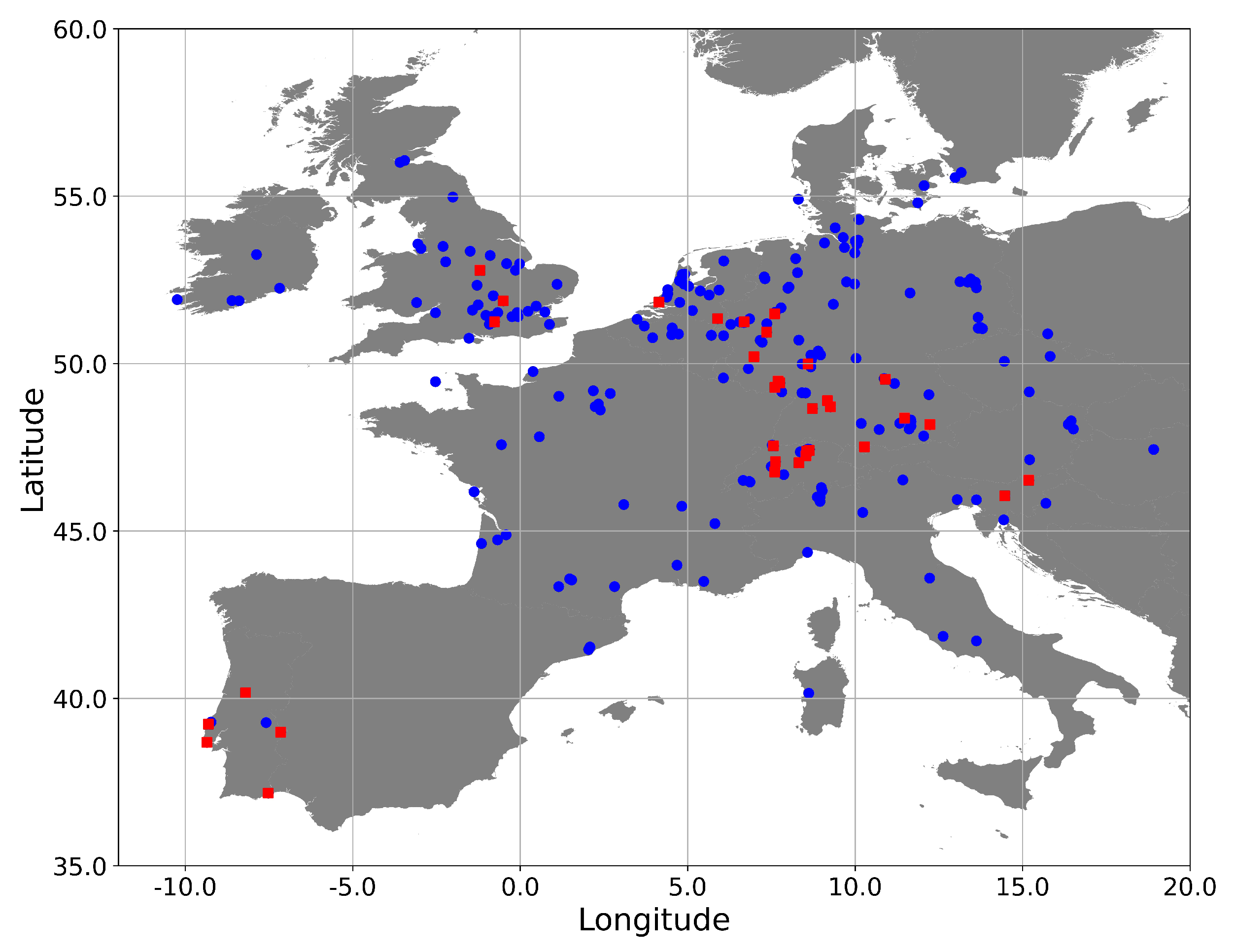
In this competition, 241 stations have been synchronized in total. The stations are randomly located in Europe, as presented in Figure 1. As mentioned above, 45 stations were marked as synchronized initially and formed two clusters. Inside each, multiple stations detected the same signal from an aircraft; stations from different clusters were too far away from each other and could not receive the same signal. The biggest cluster was located predominantly across Switzerland, Germany, Holland and England, and the smallest one was in Portugal.

Figure 1. Locations of all synchronized stations: the initial set of 35 synchronized stations is marked by red squares, all the other stations by blue circles.

As shown in the previous section, some synchronized stations were required from the beginning to synchronize other stations which experience clock drift. One can imagine an iterative process during which a new set of stations have their timestamps corrected, and these new stations are used as synchronized everywhere thereafter. Let us consider the selection of initially synchronized stations separately.

The selection of the initial set of synchronized stations will affect the quality of synchronization of all other stations. That is why it is important to create a robust initial set, in which stations meet the following criteria:

• Station location should be known with high accuracy;
• Any station should have several other synchronized stations nearby, each of which received the same aircraft signals together with a given station.

Both criteria can be checked visually. For the first one, aircraft timestamps were calculated by applying the radio wave velocity model and deducting signal time-of-flight values from stations’ timestamps. When the same signal was detected by two or more stations, it was possible to calculate the difference between an aircraft’s timestamps estimated using different stations. For the 45 synchronized stations, median absolute errors in aircraft timestamps were calculated. If a station has an incorrect location, this will result in more errors. The second criterion is required to be able to improve stations’ locations. Therefore, 35 out of 45 initially synchronized stations were selected as the initial set. Timestamps of these stations were used to optimize stations’ locations, find two parameters $A_0$ and B of the radio wave velocity model and determine stations’ constant clock shifts $\tau$. Due to computational complexity, not all timestamps were used in optimization but, instead, a random sample of $N=$ 20,000 pairs of stations i and j. The goal of optimization is to minimize the following equation:

$$\sum _{\begin{array}{c}i,j\\ i\ne j\end{array}}^N\left|d_i-d_j-\widehat{v}·\left(t_i-t_j+{\tau }_i-{\tau }_j\right)\right|\to min$$

(10)

where $d_i$ and $d_j$ are distances between a known location of an aircraft and stations’ locations, $\widehat{v}$ is effective velocity, $t_i$ and $t_j$ are stations’ timestamps, and ${\tau }_i$ and ${\tau }_j$ are stations’ constant clock shifts.

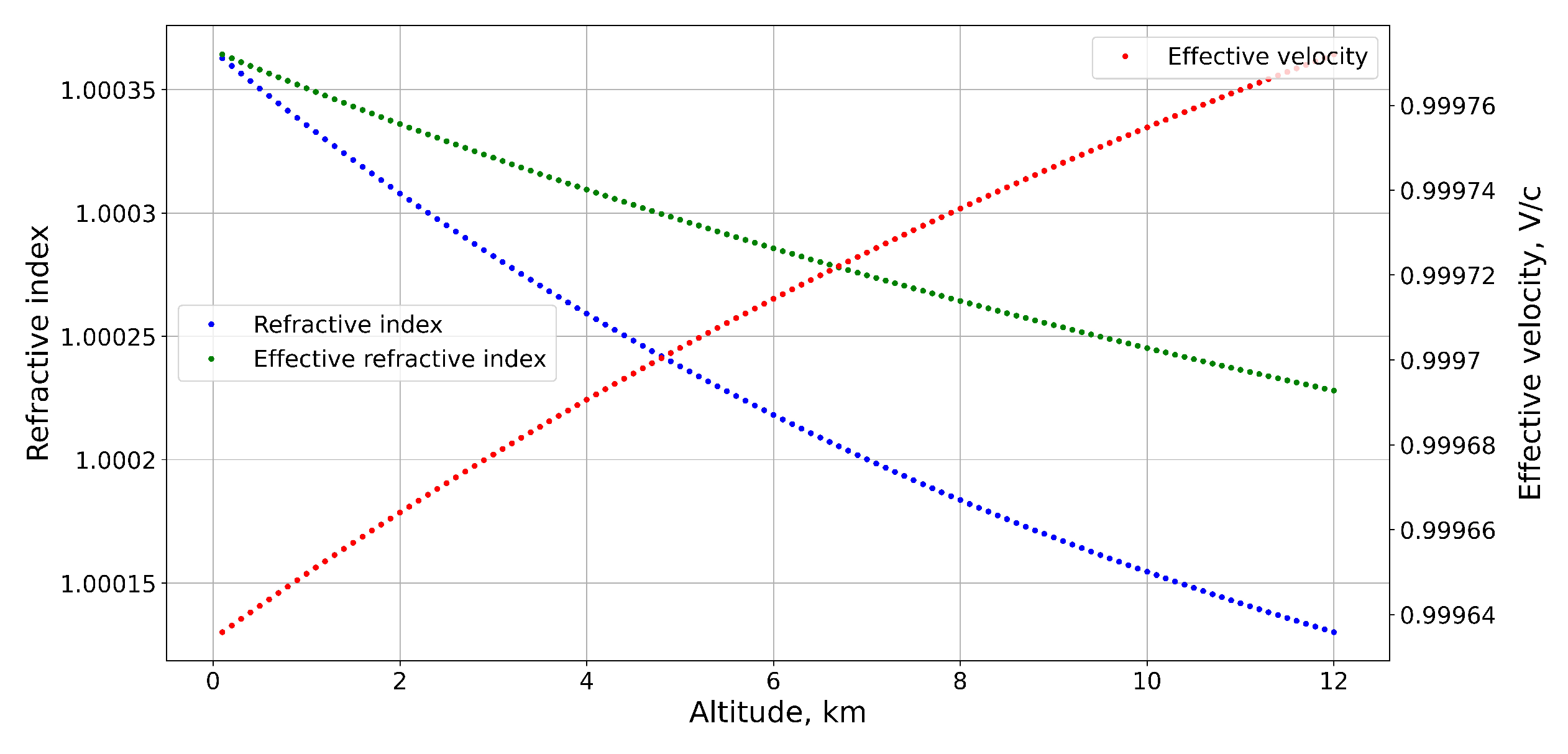
As a result, locations of the initial set of 35 stations were updated. The distance between the previous and updated locations varied from 1 m to 27 m, with average value about 10 m. Determined parameters of the radio wave velocity model allow us to investigate altitude profiles for refractive index of the atmosphere and effective radio wave velocity at different aircraft altitudes. These profiles are presented in Figure 2.

Figure 2. Altitude profiles for refractive index (blue curve), effective refractive index (green curve) and effective radio wave velocity (red curve) in the atmosphere at different aircraft altitudes. Profiles were calculated using the radio wave velocity model described in Section 2.1.

Synchronization of all other stations was made step-by-step, where, for every new station, parameters a, b and the spline were determined. Following Equation (8), linear drift of a station’s clock was fitted by a linear regression using RANSAC algorithm, which is robust to outliers. The random walk component was determined during optimization of a station’s location in Equation (9). At each optimization step, a median filter was applied to time residuals:

$$\left|t^{meas}-(a+1)·\left(t^{aircraft}+\frac{L}{\widehat{v}}\right)-b\right|$$

(11)

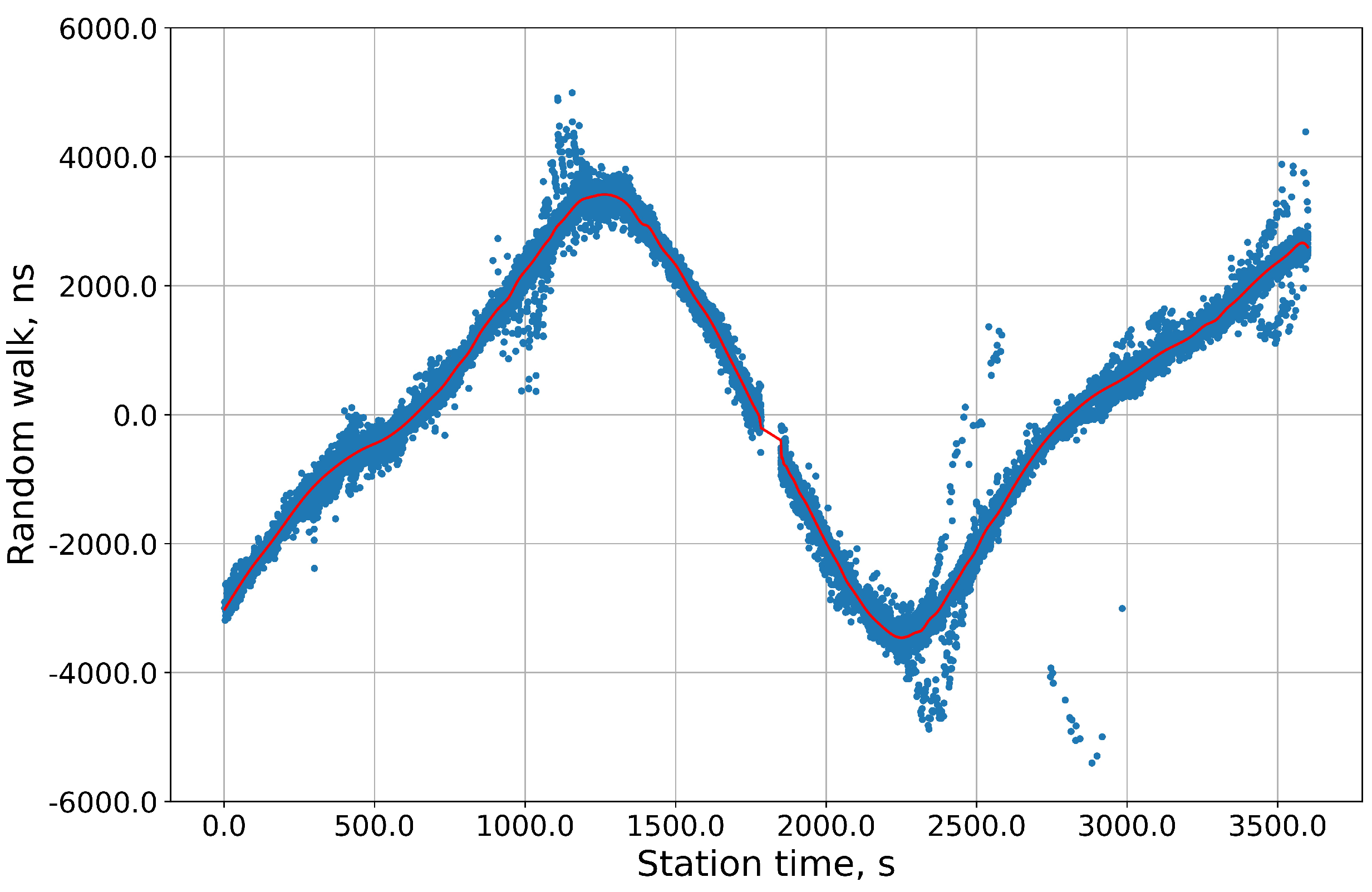
Finally, mean absolute error between time residuals and median filter output was minimized. When optimal station’s location was found, median filter output was fitted by a cubic spline. Once all components of a station’s clock drift were determined, parameters a, b and the spline coefficients and knots were saved to be able to correct the station’s timestamps at any time in the future. An example of a random walk for one station is presented in Figure 3.

Figure 3. Random walk of one station’s clock after eliminating linear clock drift. Blue points denote time residuals from Equation (11); the red solid line is a fitted cubic spline which is used to model this random walk.

2.4. Aircraft Track Reconstruction

Given a network of synchronized stations, aircraft locations could be determined using Equation (10) when timestamps from at least three stations were collected. A barycentric position for a given set of stations was used as the initial position estimation before optimization. This multilateration technique showed decent results, but, due to presence of outliers, extensive filtering of predicted aircraft locations was required.

Filtration of predicted locations was made for each aircraft separately. The main filter used in this solution was a graph-based filter developed by the winner of round one of the competition, Richard Alligier [5]. The idea of this filter is to find the longest sequence of aircraft locations where aircraft velocity does not exceed 300 m/s. The longest sequence will be a track of an aircraft. Computational complexity of the graph-based filter strongly depends on the number of input locations. Therefore, an additional filter (DBSCAN) was applied before it. DBSCAN filter joins points in clusters around core points with high density and, therefore, exclude outliers.

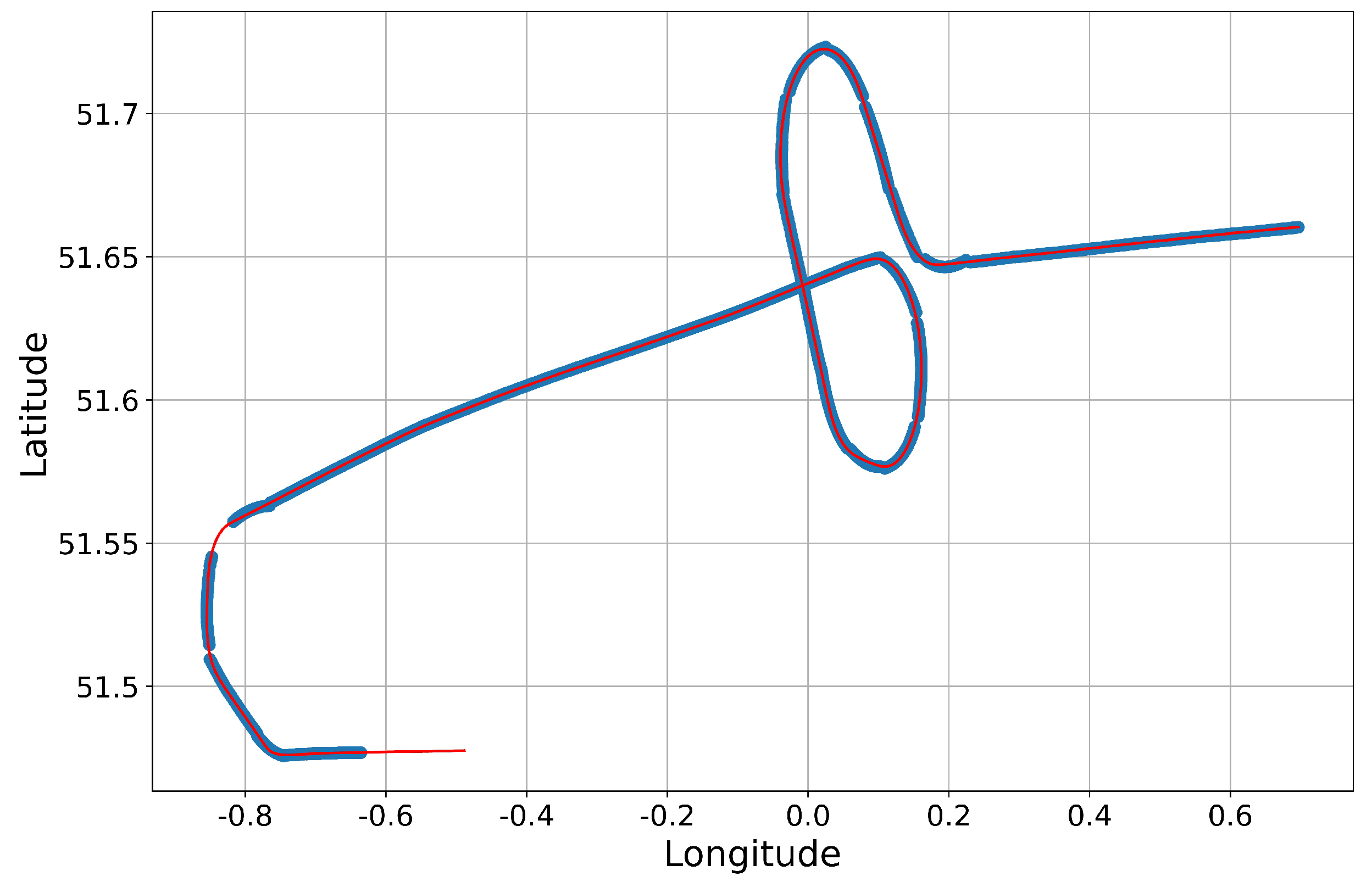
The next step in aircraft track reconstruction was predicting locations where less than three stations’ timestamps were available and to replace outliers. The author applied the method developed by him in round one. Latitude and longitude values of predicted aircraft locations were separately fitted as second order polynomial functions of aircraft time using the Huber regression algorithm within a time window of 30 s. Huber regression was used here as a robust algorithm against outliers. A minimum of 10 points within the 30 s time window were found to be required in order to achieve decent and robust results. An example of predicted aircraft track is presented at Figure 4.

Figure 4. Predicted aircraft locations (blue circles) and the ground truth (red line).

After filtering aircraft locations and the track reconstruction step, the author predicted $71.8\%$ of points in the test dataset and received about 85 m RMSE 2D distance prediction accuracy on the public leaderboard of the competition. In order to improve prediction accuracy further, we proposed two solutions: (1) remove predicted locations with the highest estimated errors; and (2) fill in small gaps between parts of the same track.

Aircraft locations predicted using the multilateration technique (initial locations) and the ones calculated during track reconstruction (reconstructed locations) give the first estimation of prediction error for initial locations. In order to get prediction error estimation for reconstructed locations, splines of order 5 were fitted to latitude and longitude values of initial locations as functions of aircraft time. Finally, prediction error for a reconstructed location was estimated as a distance to a location predicted by splines. Reconstructed locations with predicted error higher than a threshold were removed from submission. The threshold value was selected so that $70\%$ of points remain in submission.

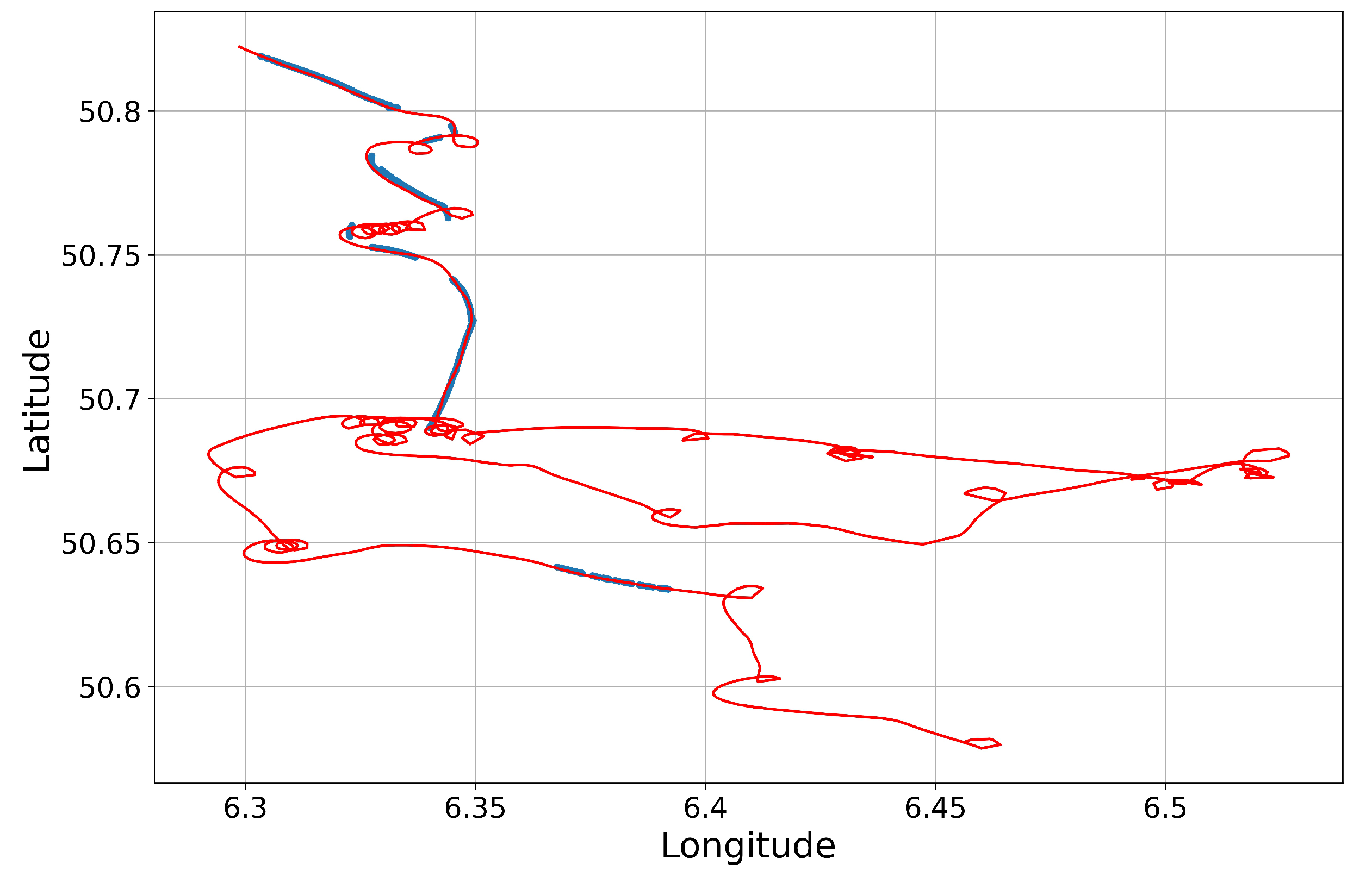
The second solution was based on an observation that small gaps and edge points of parts of a track have similar prediction errors. It was found that time gaps of 60 s or less improve total prediction accuracy when these gaps are filled with predicted locations. As a result, this solution showed 81.9 m RMSE 2D distance prediction accuracy on $70\%$ of the test dataset on the private leaderboard of the competition (78 m on the public leaderboard).

Accurate estimation of prediction error was very important for tracks like those presented in Figure 5.

Figure 5. Predicted aircraft locations (blue circles) and the ground truth (red line).

3. Conclusions

This work is focused on the synchronization of stations having strong clock drift or even providing completely broken timestamps. The methodology of synchronization of stations was developed as an iterative process starting from the initial set of synchronized stations. It includes two mathematical models for radio wave velocity in the atmosphere and the receiver clock drift model, which were presented. This methodology was tested on the competition dataset provided by the OpenSky Network, in which 241 stations were synchronized, including 35 GPS-equipped. The multilateration technique coupled with extensive filtering was applied to predict $70\%$ of aircraft locations from the test dataset with accuracy 81.9 m RMSE 2D distance.